Coupling Coordination Analysis of Livelihood Efficiency and Land Use for Households in Poverty-Alleviated Mountainous Areas

Abstract

The interaction between livelihood means and land use pattern of households is the core of the interactive coupling of the human-land system. This study focuses on Qinba mountainous area in southern Shaanxi province, a typical poverty-alleviated mountainous area. With the help of the coupling coordination degree model, kernel density estimation, and trend surface analysis, this study constructs the coupling coordination degree of livelihood efficiency and land use for households, and analyzes the differences between households’ livelihood efficiency and land use level, as well as the coupling coordination relationship between households livelihood efficiency and land use in different types and regions. The research conclusions are as follows. (1) For households in the Qinba mountainous area, southern Shaanxi province, the livelihood efficiency is at a medium level of 0.681, the land use is at a low level of 0.127, while the coupling coordination degree 0.526 is at the primary coordination state. (2) With the increase of nonagricultural degree, the coupling coordination degree of households increases first, and then decreases. (3) The coupling coordination degree for households east-to-west is “sagging”, while south-to-north diagram is “hogging”. (4) The distribution of the coupling coordination degree for agriculture-dependent households east-to-west (the “sagging” diagram) is opposite to the other types of households. By analogy, the distribution of the coupling coordination degree for nonagriculture and agriculture-dependent households north-to-south (the “hogging” diagram) is opposite to the other types of households. The coupling coordination between the households’ livelihood efficiency and land use level is affected by the households’ regional development level, natural resources, geographic location, infrastructure availability and many other factors. Making appropriate livelihood development plans based on the types of households and regional space can both effectively improve the livelihood conditions, as well as offer guidance in promoting regional human-land activity coordination and ensuring sustainable development.

1. Introduction

The human-land relationship and its evolution are key issues for rural development, and the core content of research on human-land relationship is to reveal the interaction and influence mechanism between the population system and the land system, coordinate the human-land relationship, and promote regional sustainable development [1]. At present, the tense human-land relationship and land in China’s mountainous areas, as showcased here by the Qinba mountain area in southern Shaanxi province, reveal a shortage of per capita cultivated land, its lower quality, weak agricultural infrastructure and lower economic benefits. This situation seriously restricts the development of households, preconditions the massive migration of the rural labor force, and increasingly highlights the problems in nonagricultural rural industries, obsolete production lines and poor natural resources [2]. Furthermore, with the development of urbanization, disordered development of land resources, extensive exploitation and utilization of land resources, degradation of land ecological functions have become increasingly intensified [3]. How to coordinate the relationship between households’ livelihoods and land use, promote the economical and intensive utilization of land resources, and facilitate a continuous increase in households income, has become primary issues in the development of agricultural and rural areas and the implementation of a rural revitalization policy.

The human-land relationship is an open giant system formed by the interaction of two complex systems: geographical environment and human activities. In related research, scholars have carried out research on “man”, “land” and “human-land relationship”. In terms of “man”, scholars have conducted research on livelihood capital, livelihood strategies, livelihood means, livelihood vulnerability and livelihood output, among others, mainly from the perspective of sustainable livelihood [4,5,6,7,8] and pointed out that the fundamental reasons for the backward development of rural areas are insufficient and irrational allocated livelihood capital stock, poor feasibility of livelihood means, and limited livelihood approaches [9]. To fundamentally solve the above-mentioned problems and improve the livelihood ability of the households and effectiveness of rural development, it is necessary to carry out research on efficiency evaluations that match the livelihood means to explore the process characteristics and mechanism of livelihoods [10]. In terms of “land”, scholars have mainly explored the behavior, efficiency, structure, influencing factors, and spatial-temporal differentiation of land use [11,12,13,14,15]. For regions with obvious differences in landform, such as plains, hills, and mountains, the level of intensive use of households has significant differences [16]. At the same time, the social and economic development level, policy environment, resource endowment, land fragmentation, land transfer, family characteristics of households, agricultural production subsidies, and the proportion of economic crops and other factors also have an impact on the land use level of households [17,18,19].

Livelihood reflects the selective utilization of resources by human beings [20]. The regional differentiation of the natural geographical environment and the regional differences of socio-economic conditions make human beings exhibit different resource value orientations, utilization modes and utilization levels in resource utilization [21]. As the main body of land resource utilization and protection, household livelihoods (livelihood capital, livelihood strategy, etc.) are closely related to the utilization of land resources (utilization structure, utilization efficiency, etc.). Therefore, scholars focus on the relationship between household livelihood and land use and explore this from two aspects. Some research focuses on the impact of household livelihood on land use. The evolution of livelihood capital endowments and livelihood means of households leads to changes in land use efficiency, intensity and structure [22], which also have direct or indirect impacts on the ecological environment system [23,24]. Generally speaking, households with higher human capital and natural capital are more dependent on resource utilization [25], and diversified livelihood means can help to improve land use efficiency of households and reduce livelihood risks [26]. Other research focuses on the impact of land use on the livelihoods of households. Related research focuses on analyzing the impact of land degradation, changes in land use pattern, land use type, and land use intensification on livelihood capital and livelihood strategies of households [27,28]. The change of land use mode can effectively improve the livelihood adaptability of households. There are significant differences in land use efficiency of households with different livelihood strategy types, and household diversified and nonagricultural livelihood strategies can help to improve land use efficiency and reduce livelihood risk [29]. The efficient use of land resources helps households increase their income, improve their economic status, reduce their vulnerability, improve the accessibility of assets and the sustainability of resource management [30]. On the contrary, it has a wide and profound impact on community poverty, residents’ livelihood mode, population migration and mobility [31].

In essence, the available research on human-land relationships have paid more attention to a single aspect of either livelihood or land use, and mostly discussed a one-way impact, ignoring the mutuality and interaction between the two. In addition, previous studies have mostly focused on the relationship between a single segment of livelihood (such as capital strategy or efficiency) and land use, but seldom do they explore the interaction and spatial distribution law between livelihoods and land use of households from the perspective of process and efficiency systematically. In fact, the two major subsystems of the man-land system, the livelihood system and the land use system of households, change in an interwoven way. The change in the livelihood system leads to change in the land use system, which induces further change in the livelihood system [32]. For regions with different landforms, resource endowments and economic development levels, the relationship between household livelihood and land use is also different. Especially for the Qinba Mountain Area in southern Shaanxi, a typical poverty-alleviated mountainous area, there are obvious differences between household livelihood and land use in various regions. Therefore, taking Qinba mountainous area as the research subject, this study analyzed the coupling coordination relationship between the livelihood efficiency and land use of households in different types and regions in the Qinba mountainous area by constructing a model for the coupling coordination degree of livelihood efficiency-land use of households, hoping to provide a decision-making reference for promoting the coordinated development of the livelihood and land use of households to design regional sustainable development policies.

The main contributions of this study are as follows. (1) An innovative concept of “livelihood efficiency” as the standard for evaluating household livelihood via development capacity and quality is introduced, along with a new perspective and method for sustainable livelihood research. (2) Pay attention to the mutuality and impact between household livelihood and land use practices, exploring the relationship between them from the perspective of process design and implementation efficiency, which enriches and expands the research of “human-land relationship”. (3) Starting from the household and spatial levels, we explore the coupling coordination relationship between household livelihood efficiency and land use, ensuring practical and targeted countermeasures, along with suggestions for households of different types and regions.

The next Section 2 introduces the current situation, data sources and research methods related to the Qinba mountain area in southern Shaanxi. Section 3 presents the results of household livelihood efficiency and land use intensity analyses, as well as the coupling degree, development degree, and coupling coordination degree from the perspective of household types and regional distribution. Section 4 summarizes the research, draws conclusions, and puts forward relevant solutions or countermeasures.

2. Materials and Methods

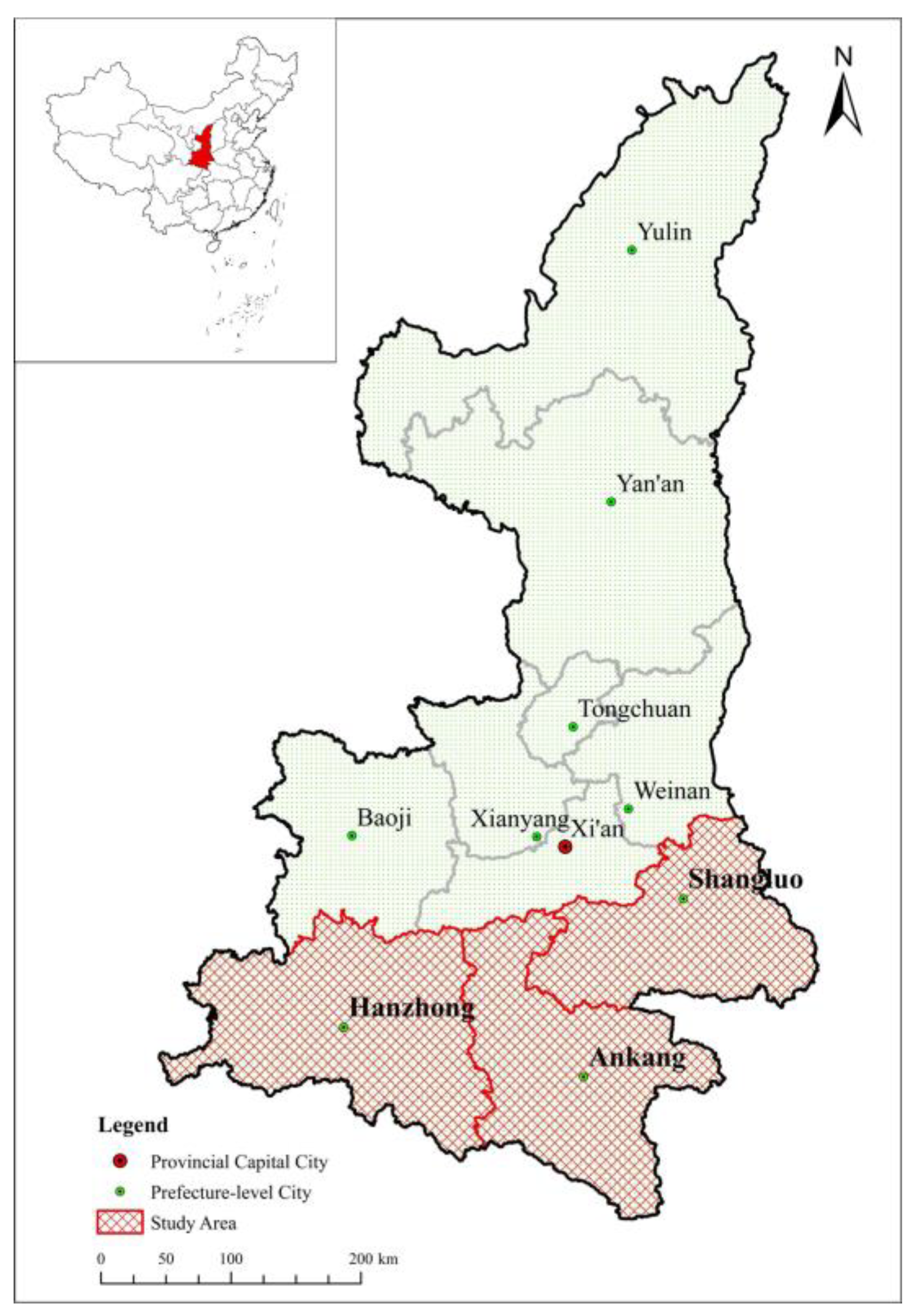
2.1. Research Area

Qinba is a 7.03 × 10⁴ km² mountainous area south of Shaanxi province (i.e., 34.19%), covering 3 cities, Hanzhong, Ankang, and Shangluo, and a total of 28 districts, as well as counties such as Ziyang, Shiquan, Zhen’an, and Ningqiang (Figure 1) [33]. As a typical poverty-alleviated mountainous area, Qinba has a complex geological structure, weak infrastructure, poor transportation network, insufficient land supply, limited income source for households, and rigid agricultural production. This has led to low livelihood capacity and efficiency for households [34,35]. As a national key ecological area, it steadily maintains the roles of “ecological security”, “resource reserve” and “landscape designer”. In order to maintain ecosystem security, households in the area have sacrificed a number of development opportunities, the utilization intensity of land resources is low, and the “rich poverty” phenomenon has become chronic in the area. Nowadays, promoting high-quality development limited by resource conservation and environmental protection policies to strike a balance between survival and development for land use by the households is an acute practical challenge in Qinba.

2.2. Data Sources

The research data reflect the results of a field household survey conducted by the research team in Qinba in August 2020. The samples of the formal survey represent the interviewee household information selected via stratified random sampling as “sample city-sample district and county-sample town-sample village-households”. A total of 796 questionnaires were collected from 24 districts and counties in the three cities of Hanzhong, Ankang, and Shangluo. This survey has two parts: household livelihood, and production (planting and breeding). A total of 746 valid data points were obtained after screening households’ livelihood data. A total of 639 valid questionnaires were obtained after screening household livelihood and production data, with an effective questionnaire rate of 80.28%. At present, the population migration from the Qinba mountain area in Southern Shaanxi is alarming. Most of the remaining rural population are the elderly and disabled groups, or people engaged in nonagricultural activities. The lack of a large number of household production statistics makes the effective questionnaire rate of this study relatively low. The basic characteristics of sample households are shown in

Table 1. Basic characteristics of sample households.

Index	Category	Frequency Number	Frequency Rate
Gender	Male	351	54.93%
	Female	288	45.07%
Age groups	≤20 years old	47	7.35%
	21–35 years old	135	21.13%
	36–50 years old	259	40.53%
	51–65 years old	143	22.38%
	≥66 years old	55	8.61%
Education level	Primary school and lower	224	35.05%
	Junior high school	212	33.18%
	High school or technical secondary school	89	13.93%
	Junior college or higher	114	17.84%
Population size	≤2	42	6.57%
	3–4	391	61.19%
	≥5	206	32.24%

. It can be seen from Table 1 that this survey covered households of different age groups, and the ratio of males and females was basically equal, among which 68.23% received education not exceeding junior high school. By comparing the survey data against the statistical data of Shaanxi province, Hanzhong city, Ankang city, Shangluo city, it can be concluded that the samples obtained are consistent with the actual local conditions, and thus representative to a certain extent.

2.3. Variable Selection

2.3.1. The Evaluation Index System of Household Livelihood Efficiency

Livelihood efficiency reflects the feasibility of households to survive and seek development, which is a comprehensive reflection of the allocation status, utilization effect and management decision-making level of the capital elements that are used for the livelihood of households in their livelihood activities [36]. Based on the research results of household livelihoods [37,38,39] and the actual conditions of households in Qinba, this study constructed an evaluation index system of household livelihood efficiency (

Table 2. The evaluation index system of household livelihood efficiency.

Evaluation Index		Variable	Definition and Description of Variable
Livelihood input	Human capital	Age	0.5: ≤20 years old; 2: 21–35 years old; 3: 36–50 years old; 1.5: 51–65 years old; 0.8: ≥66 years old
		Education level	1: Primary school and lower; 2: Junior high school; 3: High school or technical secondary school; 4: Junior college or higher
		Health status	1: very bad; 2: bad; 3: fair; 4: good; 5: very good
		Population size	Number of family members
	Physical capital	Number of livestock	0: 0; 1: 1–10; 2: 11–20; 3: 21–30; 4: ≥31
		Daily supplies	Quantity of daily supplies (pieces)
		Transportation/vehicle tools	Number of transportation/vehicle units (vehicles)
		Housing condition	Number of rooms (rooms)
	Natural capital	Cultivated land area	Gross cultivated land area (mu)
		Planting area	Actual planting area (mu)
		Whether production water can be used as domestic water	0: no; 1: yes
	Financial capital	Gross annual income	1: 10,000 and below; 2: 10,000–20,000; 3: 20,000–50,000; 4: 50,000–100,000; 5: more than 100,000
		Loan/money borrowing opportunities	0: no; 1: yes
		Channels for obtaining loans/borrowing funds	Number of channels for obtaining funds
	Social capital	Whether family has cadres	0: no; 1: yes
		Trust of neighbors and villagers	1: Almost none; 2: Minority; 3: Half; 4: Majority; 5: Almost all
		Channels for getting help in time of livelihood difficulties	Number of channels for getting help
		Participation in the election of village cadres	0: no; 1: yes
	Information capital	Number of information obtaining devices	Number of devices used to obtain information
		Channels for obtaining information	Number of channels for obtaining information
		Timely acquisition of policy, market and other information	0: no; 1: yes
Livelihood output	Income level	Income change condition	1: Significantly reduced; 2: Reduced; 3: No change; 4: Improved; 5: Significantly improved
	Welfare level	Improvement of education and medical care	1: Significantly reduced; 2: Reduced; 3: No change; 4: Improved; 5: Significantly improved
	Employment opportunities	Improvement of employment channels	1: Significantly reduced; 2: Reduced; 3: No change; 4: Improved; 5: Significantly improved
	Rural attachment	Sense of pride and attachment to hometown	1: Significantly reduced; 2: Reduced; 3: No change; 4: Improved; 5: Significantly improved
	Ecological protection consciousness	Ecological protection consciousness and values	1: Significantly reduced; 2: Reduced; 3: No change; 4: Improved; 5: Significantly improved

) using livelihood input (human capital, physical capital, natural capital, financial capital, social capital, and information capital) as the input index, and livelihood output (income level, welfare level, employment opportunities, rural attachment, ecological protection awareness) as the output index.

2.3.2. Evaluation Index System of Household Land Use Level

Based on the related research results for land use [40] and the actual land use conditions for households in Qinba, this study constructed the evaluation index system of household land use level (

Table 3. The evaluation index system of household land use level.

Evaluation Index		Variable	Definition and Description of Variable
Land use level	Land use intensity	Per capita cultivated land area	Gross cultivated land area/gross family population (mu/person)
		Irrigation condition	0: no; 1: yes
		Idle land	0: no; 1: yes
		Land circulation	0: no; 1: yes
	Land use structure	Agricultural structure	1: No planting and no breeding; 2: Only planting; 3: Only breeding; 4: Planting and breeding
		Land input	Gross planting and breeding area (mu)
		Labor input	Number of labor force aged 20–65 (person)
		Funds input	Input cost of seeds, pesticides, chemical fertilizers, agricultural film, machinery (yuan)
	Land use benefits	Gross agricultural output value	Gross income from planting and breeding (yuan)
		Gross agricultural output	Gross output of planting and breeding (jin)
	Land use trend	Changes in planting labor input	1: Decrease; 2: Unchanged; 3: Increase
		Changes in planting capital input	1: Decrease; 2: Unchanged; 3: Increase
		Changes in breeding labor input	1: Decrease; 2: Unchanged; 3: Increase
		Changes in breeding capital input	1: Decrease; 2: Unchanged; 3: Increase

) from the perspective of the land use intensity, land use structure, land use benefits, and land use trends.

2.4. Research Methods

2.4.1. Coupling Coordination Degree Model

The coupling coordination degree model was introduced to analyze the coupling coordination relationship between household livelihood efficiency and land use levels to effectively reveal the interdependence and restriction mechanism between the two. In the model, the coupling degree reflects the degree of interdependence and interaction of livelihood efficiency system vs. land use system, the development degree reflects the overall benefit or level of livelihood efficiency system vs. land use system, and the coupling coordination degree refers to the degree of benign coupling in the interaction of the two systems, which can reflect the degree of coordinated development of livelihood efficiency system vs. land use system [41,42]. With reference to previous research [43,44,45,46], the coupling degree, development degree, and coupling coordination degree of household livelihood efficiency and land use can be divided into the following grades (

Table 4. Grade division standard for coupling degree, development degree, and coupling coordination degree.

Coupling Degree	Coupling Type	Development Degree	Development Type	Coupling Coordination Degree	Coupling Coordination Type
0–0.199	Severe uncoupling	0–0.199	Severe lag	0–0.199	Severe incoordination
0.200–0.399	Slight uncoupling	0.200–0.399	Slight lag	0.200–0.399	Slight incoordination
0.400–0.599	Primary coupling	0.400–0.599	Primary development	0.400–0.599	Primary coordination
0.600–0.799	Intermediate coupling	0.600–0.799	Intermediate development	0.600–0.799	Intermediate coordination
0.800–1.000	Advanced coupling	0.800–1.000	Advanced development	0.800–1.000	Advanced coordination

).

2.4.2. Kernel Density Estimation

Kernel density estimation is mainly used to estimate the probability density of random variables. Continuous density curves are used to describe the distribution pattern of the random variables to reveal the evolution trend of differences intuitively [47,48]. Stata16 software was used to draw a kernel density map to clarify the distribution characteristics of the coupling coordination relationship between household livelihood efficiency and land use at the household level.

2.4.3. Trend Surface Analysis

The trend surface is an approximate treatment of the actual surface, which represents the spatial distribution law and change trend of geographic elements or observed value [49,50]. With the help of the trend surface analysis tool in ArcGIS software, we explored the overall spatial differentiation trend of the coupling coordination relationship between household livelihood efficiency and land use.

3. Results

Based on the household livelihood efficiency measured using the DEA model and the household land use level measured with the entropy method, we obtained statistical results of the coupling coordination between household livelihood efficiency and land use with the aid of the coupling coordination degree model.

Table 5. Statistics for coupling coordination between household livelihood efficiency and land use.

Item	Category	Sample Size	Minimum Value	Maximum Value	Average Value	Standard Deviation
Livelihood efficiency	Comprehensive efficiency	639	0.298	1.000	0.681	0.178
	Pure technical efficiency	639	0.342	1.000	0.759	0.184
	Scale efficiency	639	0.487	1.000	0.903	0.111
Land use	Land use level	639	0.013	0.838	0.127	0.065
Coupling coordination	Coupling degree	639	0.274	1.000	0.705	0.136
	Development degree	639	0.195	0.790	0.404	0.091
	Coupling coordination degree	639	0.307	0.888	0.526	0.070

shows the overall condition of livelihood efficiency, land use level, coupling degree, development degree, and coupling coordination degree of households in Qinba.

Table 5 shows the coupling coordination between livelihood efficiency and land use of households in Qinba.

(1)

Livelihood efficiency. Using DEAP2.1 software to calculate the household livelihood efficiency, the average values of comprehensive efficiency, pure technical efficiency and scale efficiency are 0.681, 0.759, and 0.903, respectively, based on which, it can be concluded that the livelihood efficiency (comprehensive efficiency) of households in Qinba is at a relatively medium level. Comparatively speaking, the comprehensive efficiency value is at its lowest, which indicates that various livelihood capital of households in Qinba have not been optimally allocated, and there is still much opportunity for improvement in livelihood efficiency. The scale efficiency of households is at a relatively high level, which indicates that the overall effect and scale of the input and output for local households is good.

(2)

Land use level. The minimum, maximum and average land use level of households in Qinba are 0.013, 0.838, and 0.12,7 respectively, which indicates that the overall land use level by local households is quite different and low.

(3)

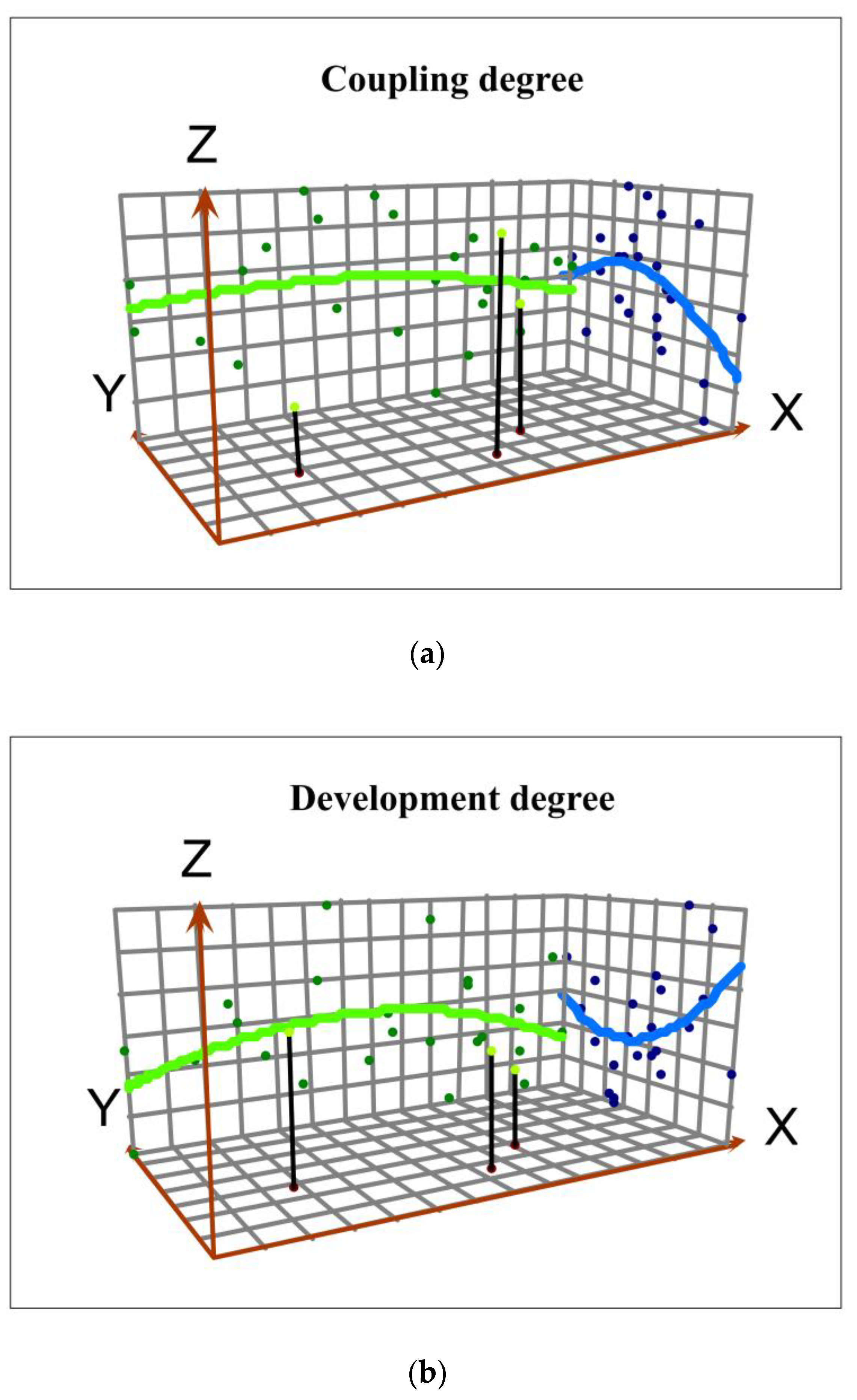
Coupling degree. The average coupling degree between livelihood efficiency and land use of households in Qinba is 0.705. The overall coupling degree is at the intermediate coupling state, indicating a high degree of interaction between household livelihood efficiency and land use.

(4)

Development degree. The average development degree of livelihood efficiency and land use development of households in Qinba is 0.404. The overall development degree is at the primary development state, which indicates that the overall development level of household livelihood efficiency and land use is relatively poor.

(5)

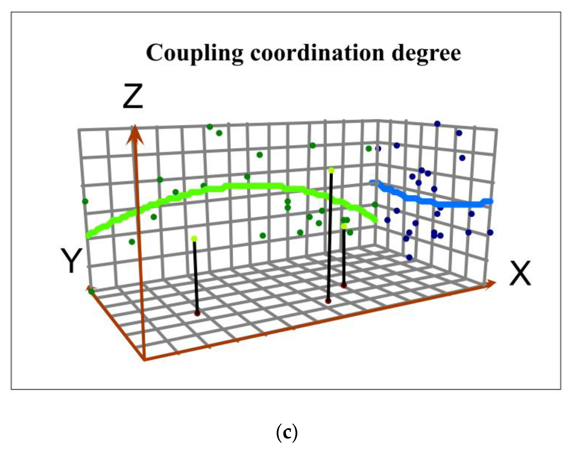
Coupling coordination degree. The average coupling coordination degree between livelihood efficiency and land use of households in Qinba is 0.526. The overall coupling coordination degree is at the primary coordination level, which indicates a relatively low degree of the benign influence as well as the benign coupling of household livelihood efficiency and land use.

In a sense, the overall livelihood efficiency of households in Qinba is relatively high, but the overall land use level of households is low, which weakens the coupling coordination between the local household livelihood efficiency and land use to some extent. In the future, more attention needs to be paid to the land use practice by the households so as to promote the sustainable, coordinated, and high-quality development of their livelihood and land use levels.

3.1. Analysis of the Differences in Household Livelihood Efficiency

With reference to previous research [51,52], this study divided households into four types, namely pure-agriculture households, agriculture-dependent households, nonagriculture-dependent households and nonagriculture households according to the nonagriculturalization degree (the proportion of nonagricultural income to gross income was 0–10%, 10–50%, 50–90% and 90–100%, respectively). It was found that the difference in livelihood efficiency of different types of households in Qinba is small, and they are all at a relatively medium level. Specifically speaking, the pattern of livelihood efficiency of various types of households is: nonagriculture households (0.692) > pure-agriculture households (0.688) > agriculture-dependent households (0.674) > nonagriculture-dependent households (0.648). In other words, with increase in the nonagricultural degree, the livelihood efficiency of households decreases at first, and then increases, the distribution being “U-shaped”. The livelihood efficiency of the specialized (pure-agriculture, nonagriculture) households is higher than that of dependent (agriculture-dependent, nonagriculture-dependent) households, which means that one-way production concentrates on resource utilization to improve livelihood efficiency, while diversified production methods may lead to over-dispersion of resource utilization and reduce livelihood efficiency.

ArcGIS software was used to explore the spatial distribution pattern and distribution law of households’ livelihood efficiency. Comparing the livelihood efficiency of households in different regions (cities), it can be concluded that the livelihood efficiency of households in Hanzhong city is the highest (0.695), followed by Shangluo city (0.679) and Ankang city is the lowest (0.673). From the perspective of districts and counties, the livelihood efficiencies of households in Lueyang county, Yang county, Shiquan county, Zhen’an county, and Shanyang county are relatively low, and those of households in Zhenba county and Langao county are relatively high. Using the trend surface analysis tool, it can be seen that the livelihood efficiency of households shows an “inverted U-shaped” structure, i.e., high in the middle and low on both sides, from east to west. The curvature is small, which means that the difference in the livelihood efficiency of households from east to west is small. The livelihood efficiency of households shows a “U-shaped” pattern, i.e., low in the middle and high on both sides, from south to north. The curvature is relatively large, and the livelihood efficiency of households in the southern region is significantly higher than that in the northern region. This is mainly because the geographic environment, terrain and landform have a certain impact on their livelihood efficiency. From the perspective of topography, Hanzhong city is high in the north and low in the south, Ankang city is high in the north and south, and low in the middle, while Shangluo city is high in the northwest and low in the southeast. Compared with the low mountain plain area, the mountainous area has complex terrain, poor traffic conditions and weak infrastructure. The geographical environment results in the relatively poor livelihood ability and livelihood efficiency. For example, the distribution characteristics of livelihood efficiency is opposite to its topographic characteristics for households in Hanzhong city, which shows the characteristics of being low in the north and high in the south from south to north. In addition, the geographic location and the regional social and economic development level also have an impact on the efficiency livelihood. For example, as the political and economic development center of Shangluo city, Shangzhou district is close to Xi’an. The superior geographical location contributes to the relatively high livelihood efficiency.

3.2. Analysis of the Differences in Household Land Use Level

The difference in land use level of different types in Qinba is small, and they are all at a relatively low level. Specifically speaking, the land use levels of various types of households show the following pattern: agriculture-dependent households (0.162) > pure-agriculture households (0.159) > nonagriculture-dependent households (0.134) > nonagriculture households (0.114). In other words, with the increase in the nonagricultural degree, the land use level of households increases first, and then decreases, the distribution of which is an inverted U-shape. It was found that the land use level of agriculture-dependent households is higher than that of the pure-agriculture households. This is because that agriculture-dependent households may constantly adjust their land use structure to take into account both agricultural and nonagricultural production activities, and the nonagricultural income can be further invested in agricultural production to improve the land use level. However, due to the limitation of land area, land quality, market prices and other factors, for pure-agriculture households, it is difficult to improve their land use efficiency, which results in the lower land use level.

The land use level of households in Qinba is at a relatively low level, among which the land use level of households in Hanzhong city is the highest (0.137), followed by Ankang city (0.124), and Shangluo city is the lowest (0.119). From the dimension of districts and counties, the land use levels of households in Lueyang county, Mian County, Hanyin County, Shangzhou District, and Langao county are lower, while those of households in Yang county, Xixiang county, Shiquan county, and Ziyang county are higher. From east to west, the land use level of households presents an inverted U-shape pattern, high in the middle and low on both sides, with a relatively large curvature, that is, the land use level of households in the central region is significantly higher than that in the eastern and western regions. From north to south, the land use level of households is in an inverted U-shape pattern, high in the middle and low on both sides, and the curvature is small, that is, the difference in land use level of households from east to west is small. Affected by the terrain and landscape, in areas with higher terrain such as Lueyang county and Mian County, the complex terrain, surface relief, and the land fragmentation restrict the intensive use of land resources by households and weakens the land use level by households. In the lower terrain areas such as Xixiang county and Shiquan county, the flat and wide land is more convenient for households to engage in agricultural production and large-scale operations, so the land use level is higher.

3.3. Coupling Coordination Relationship between Different Types of Household Livelihood Efficiency and Land Use

Different types of households have certain differences in the selection and combination of livelihood strategies, and possession and utilization of land resources, which differentiates the coupling coordination relationship between different types of household livelihood efficiency and land use. To this end, this study starts from the type of households to further analyze the difference characteristics of the coupling coordination relationship between livelihood efficiency and land use at the household level. Among them,

Table 6. Statistical results of the coupling coordination between different types of household livelihood efficiency and land use.

	Livelihood Efficiency	Land Use Level	Coupling Degree	Development Degree	Coupling Coordination Degree	Sample Size	Percentage
Pure-agriculture households	0.688	0.159	0.741	0.424	0.552	78	12.21%
Nonagriculture-dependent households	0.674	0.162	0.759	0.418	0.558	39	6.10%
Nonagriculture-dependent households	0.648	0.134	0.724	0.391	0.525	137	21.44%
Nonagriculture households	0.692	0.114	0.685	0.403	0.518	385	60.25%

shows the statistical results of the coupling coordination between different types of household livelihood efficiency and land use, and Figure 2 shows a kernel density estimation diagram of the coupling coordination relationship between livelihood efficiency and land use of different types of households.

3.3.1. Coupling Degree Analysis of Different Types of Households

It can be seen from Table 6 that the coupling degree between the livelihood efficiency and land use of various types of households in Qinba is at an intermediate coupling state. The comparison shows that the coupling degree of various types of households presents the following pattern: agriculture-dependent households (0.759) > pure-agriculture households (0.741) > nonagriculture-dependent households (0.724) > nonagriculture households (0.685). That is to say, with the increase in the nonagriculturalization degree, the coupling degree of households increases first, and then decreases, the distribution of which is an inverted U-shape. It was found that the coupling degree of agriculture-dependent households is always higher than that of specialized households in agricultural and nonagricultural production activities, that is, the coupling degree of agriculture-dependent households is always higher than that of pure-agriculture households, and the coupling degree of the nonagriculture-dependent households is higher than that of the nonagriculture households. This is because compared with pure-agricultural households, nonagriculture households and other specialized households, the livelihood activities of agriculture-dependent households involve agricultural activities and nonagricultural activities. A diversified livelihood means draws the household livelihood system and the land system closer, which in turn increases the coupling degree of agriculture-dependent households.

Judging from the kernel density estimation diagram of the coupling degree between livelihood efficiency and land use in Figure 2, the coupling degree is different for various types of households. Comparing the curves of various types of households, it can be seen that the peaks of nonagricultural households are the steepest, indicating that the land use level concentration of nonagricultural households is the highest. The curves of various types of households all show a left-skewed distribution, indicating that there is a difference in the coupling degree of households, and the coupling degree of various types of households is mostly at a higher level. The main reason is that the livelihood activities of nonagricultural households are mainly nonagricultural activities, and the land use level is smaller, and the mutual influence and interaction between the household livelihood system and the land system are smaller and relatively concentrated, while the livelihood activities of pure-agricultural households, agriculture-dependent households and nonagricultural-dependent households all involve the use of land resources. The difference in land use levels results in the relationship between different types of household livelihood systems and land systems showing different development trends.

3.3.2. Development Degree Analysis of Different Types of Households

It can be seen from Table 6 that the development degree between the livelihood efficiency and land use are different for various types of households in Qinba. Among them, the development degree of nonagriculture-dependent households is at the slight lag state, and the development degree of pure-agricultural households, nonagricultural households, and agriculture-dependent households is at the primary development state. Specifically, the development degree of various types of households presents the following pattern: pure-agricultural households (0.424) > agricultural-dependent households (0.418) > nonagricultural households (0.403) > nonagriculture-dependent households (0.391). That is to say, with the increase in the nonagriculturalization degree, the development degree of households decreases first, and then increases, the distribution of which is U-shaped. It was found that in the agricultural and nonagricultural production activities, and the development degree of the specialized households, is always higher than that of the agriculture-dependent households. The development degree of pure-agriculture households is higher than that of agriculture-dependent households, and the development degree of nonagriculture households is higher than that of nonagriculture-dependent households. This is because specialized households tend to use one or several resources to maximize their benefits. The centralized development strategy enables households to effectively use resources and increase their overall benefits, while agriculture-dependent households tend to use multiple resources to maximize the benefits. However, due to the limitations of education, resources, and technology, households have insufficient resource management levels, which limits their overall benefits.

Judging from the kernel density estimation diagram of the development degree between livelihood efficiency and land use in Figure 2, the development degree is different for various types of households. Comparing the curves of various types of households, the peaks of nonagriculture-dependent households are the steepest, followed by agriculture-dependent households and nonagriculture households. The curve of pure-agricultural households is the flattest, indicating that the concentration of development degree of the nonagriculture-dependent households is the highest while the differentiation of the pure-agricultural households is the largest. It can be seen from the shape of the curve that the pure-agricultural households show a significant right-skewed distribution with a longer tail, indicating that there is a large gap in the development degrees among the pure-agricultural households indicating a state of polarization, with most of them at a low-medium level. In addition, the curves of nonagricultural-dependent households and nonagricultural households also show a right-skewed distribution with two peaks, indicating that the development degree of nonagricultural-dependent households and nonagricultural households are at a state of polarization, but with a smaller degree of differentiation. This is because under the restrictions and driving force of land, technology, capital and population, the livelihood efficiency and land use level of pure-agricultural households are obviously polarized, resulting in a state of polarization of the overall benefit and level of pure-agricultural households, i.e., the development degree is polarized. At the same time, the difference in nonagricultural income has polarized the livelihood efficiency of nonagricultural-dependent households and nonagricultural households and further differentiated the development of households.

3.3.3. Coupling Coordination Degree Analysis of Different Types of Households

It can be seen from Table 6 that the coupling coordination degree of the livelihood efficiency and land use of various types of households in Qinba is at a primary coordination state. The comparison shows that the coupling coordination degree of various types of households presents a pattern of agriculture-dependent households (0.558) > pure-agriculture households (0.552) > nonagriculture-dependent households (0.525) > nonagricultural households (0.518). That is to say, with the increase in the nonagriculturalization degree, the coupling coordination degree of households increases first, and then decreases, the distribution of which is an inverted U-shape. The coupling coordination degree of agriculture-dependent households is always higher than that of the specialized households in agricultural and nonagricultural production activities, i.e., the coupling degree of agriculture-dependent households is always higher than that of pure-agriculture households, and the coupling degree of the nonagriculture-dependent households is higher than that of the nonagriculture households. In addition, the coupling coordination degree of pure-agricultural households and agriculture-dependent households is higher than the average level (0.526), and the coupling coordination degree of nonagricultural households and nonagriculture-dependent households is lower than the average level. This is because compared with specialized households, agriculture-dependent households comprehensively use all resources from agriculture and nonagriculture, and the comprehensive and coordinated use of multiple resources also raises the coupling coordination degree of the livelihood efficiency and land use of agriculture-dependent households. The main resource of pure-agricultural households and agriculture-dependent households’ production activities is only their land resources. Coordinating the use of land resources and other resources is the basic activity of households. Long-term practice and experience raise the coupling coordination degree of households.

Judging from the kernel density estimation diagram of the coupling coordination degree between livelihood efficiency and land use in Figure 2, the coupling coordination degree is different for various types of households, but the difference is small. Comparing the curves of various types of households, the peaks of pure-agricultural households and nonagricultural households are steeper, and the peaks of agriculture-dependent households and nonagriculture-dependent households are flatter, indicating that the concentration of coupling coordination degree of pure-agricultural households and nonagricultural households is relatively high, and the coupling coordination degree of agriculture-dependent households and nonagricultural-dependent households is highly differentiated. The pure-agricultural household curve has a significant right-skewed distribution, indicating that the coupling coordination degree of pure-agricultural households is polarized, and the coupling coordination degree of households is mainly concentrated at the middle level. The curve of agriculture-dependent households has a significant left-skewed distribution, indicating that the coupling coordination degree of agriculture-dependent households shows a gap, and most of them are at an intermediate level. This is because nonagricultural households are mainly engaged in nonagricultural activities, and their use of land resources is smaller, which makes the coupling coordination degree of households more concentrated. Affected by plantation structure, culturing structure, and land resources, pure-agricultural households have a certain degree of differentiation in the process of coordinating the use of various resources, resulting in a polarized coupling coordination degree. Nonagricultural-dependent households and agricultural-dependent households may comprehensively use land resources and other resources, and the differences of resource utilization cause differentiation in the coupling coordination degree of households.

3.4. Coupling Coordination Relationship between Household Livelihood Efficiency and Land Use in Different Regions

Affected by specific environment, and social and cultural factors, the spatial characteristics and patterns of household livelihood efficiency and land use level in various regions also vary. To this end, this study starts from a regional perspective to further analyze the characteristics of the spatial differences in the coupling coordination relationship between household livelihood efficiency and land use.

Table 7. Statistical results of the coupling coordination between household livelihood efficiency and land use in different regions (cities).

	Livelihood Efficiency	Land Use Level	Coupling Degree	Development Degree	Coupling Coordination Degree	Sample Size	Percentage
Ankang city	0.673	0.124	0.698	0.398	0.520	272	42.56%
Hanzhong city	0.695	0.137	0.721	0.416	0.541	195	30.52%
Shangluo city	0.679	0.119	0.697	0.399	0.520	172	26.92%

shows the statistical results of the coupling coordination between household livelihood efficiency and land use in different regions (cities).

The Table 7 shows the coupling coordination degree of household livelihood efficiency and land use in Ankang city, Hanzhong city, and Shangluo city in Qinba. (1) Coupling degree. The coupling degree of households in Qinba mountainous area in Southern Shaanxi is at an intermediate coupling state. Among them, the coupling degree of households in Hanzhong city is the highest (0.721), followed by Ankang city (0.698), and Shangluo city is the lowest (0.697). (2) Development degree. The development degrees of households are different in Qinba. Among them, the households of Hanzhong city have the highest development degree (0.416) and are at the primary development state. The households of Shangluo city are second (0.399), and are at the slight lag state. The households of Ankang city have the lowest development degree (0.398), and are at the slight lag state. (3) Coupling coordination degree. The coupling coordination degree of households in Qinba is at a primary coordination state. Among them, the coupling coordination degree of households in Hanzhong city is the highest (0.541), and Ankang city and Shangluo city are basically the same (Ankang city is slightly higher). In general, the coupling degree, development degree, and coupling coordination degree of households in Hanzhong city are significantly higher than those of Ankang and Shangluo, while the difference between the households in Ankang and Shangluo is smaller. The main reason is that the plain area of Hanzhong city is larger compared with those of Ankang city and Shangluo city. This brings more convenience to local social and economic development and land resource utilization.

In order to further analyze the characteristics of households at the regional level, this study used ArcGIS software to visually analyze the data of 24 sample districts and counties in Qinba, and used trend surface analysis tools to further analyze the trend of the overall differentiation in space of coupling coordination relationship between household livelihood efficiency and land use. Figure 3 is a spatial distribution diagram of the coupling coordination relationship between household livelihood efficiency and land use in different regions (districts and counties), and Figure 4 is a trend surface diagram of the coupling coordination relationship between household livelihood efficiency and land use in different regions (district and county).

3.4.1. Coupling Degree Analysis of Households in Different Regions

Figure 3 and Figure 4 show that the coupling degree of households in Qinba is concentrated in the range of 0.574–0.792, at the primary coupling state and the intermediate coupling state. The coupling degree of households in Langao county is at the primary coupling state, and the coupling degrees of households in other districts and counties are at the intermediate coupling state. In comparison, the coupling degree of households in Langao county and Pingli county is relatively low, and the coupling degree of households in Yang county, Xixiang county, Shiquan county, and Ziyang county is relatively high. The coupling degree of households presents an inverted U-shaped pattern, high in the middle and low on both sides, from east to west. The curvature is small, and the areas with high coupling degree are concentrated in the junction area of Hanzhong city and Ankang city. The coupling degree of households from north to south shows an inverted U-shaped pattern, high in the middle and low on both sides, with a relatively large curvature, and the coupling degree of households in the northern district is significantly higher than that in the southern district. In general, the spatial coupling degree is in a pattern of high in the middle and low on both sides.

This is because in high terrains such as Langao county and Pingli county, the land use level of households is lower, and the relationship between household livelihood activities and land use is weaker, resulting in a lower coupling degree. In the lower terrain areas, such as Xixiang county, the land use level of households is relatively higher, and the link between household livelihood and land use is also closer.

3.4.2. Development Degree Analysis of Households in Different Regions

Figure 3 and Figure 4 show that the development degree of households in Qinba is concentrated in the range of 0.375–0.504, at the slight lag state and the primary development state. The development degrees of households in Lueyang county, Zhen’an county, Shanyang county, Yang county, Baihe county, Shiquan county, Danfeng county, XunYang county, Zhenping county, and Hanbin District are at the slight lag state, and the development degrees of other districts and counties of households are at the primary development state. In comparison, the development degrees of households in Lueyang county, Zhen’an county, and Shanyang county are relatively lower, while the development degrees of households in Zhenba county and Langao county are relatively higher. The development degree of households shows an inverted U-shaped pattern, high in the middle and low on both sides, from east to west. The curvature is small. The development degree of households from north to south shows a U-shaped pattern, low in the middle, high on the sides, and the development degree of households in the southern district is significantly higher than that in the northern district.

The main reason is that the households’ land use level and livelihood efficiency are relatively lower in areas with higher terrain and lower levels of economic development, resulting in a lower household development degree, while in areas with lower terrain and higher levels of economic development, household land use level and livelihood efficiency are relatively higher resulting in a higher household development degree.

3.4.3. Coupling Coordination Degree Analysis of Households in Different Regions

Figure 3 and Figure 4 show that the coupling coordination degree of households in Qinba is concentrated in the range of 0.479–0.583, and they are all at a primary coordination state. The coupling coordination degree of households in Lueyang county is relatively lower, and the coupling coordination degrees of households in Xixiang county, Zhenba County, Ziyang county, Zhashui county, and Luonan county are relatively higher. The coupling coordination degree of households shows an inverted U-shaped pattern, high in the middle and low on both sides, from east to west. The curvature is relatively large, that is, the coupling coordination degree of households in the central region is significantly higher than those in the eastern and western regions. The coupling coordination degree of households from north to south shows a U-shaped pattern, low in the middle, high on the sides, and the curvature is small, that is, the difference of coupling coordination degree of households from north to south is small.

This is because in areas where the development trend of household livelihood efficiency and land use level are the same, the household coupling coordination degree shows a similar development pattern. On the one hand, household livelihood means and land use methods continue to be adjusted and optimized, which helps in building a virtuous circle with the household livelihood system and the land use system. On the other hand, due to the constraints of resource endowments, geographic environment and education level, it is difficult for households to achieve the effective allocation of livelihood resources, and the coupling coordination level between households’ livelihoods and land is also relatively lower. For example, the coupling coordination degree of households shows a development trend similar to that of the livelihood efficiency and land use level from east to west (inverted U-shaped). In areas where the development trend of household livelihood efficiency and land use level is opposite, the coupling coordination degree is affected by the combined effect of the livelihood efficiency and land use level, and present different characteristics. On the one hand, with reduction of the importance of land resources, the land use level is an important loop that reflects the benign relationship between household livelihoods and land use, and it has a relatively large impact on the coupling coordination degree of households. On the other hand, social resources, information resources and financial resources have a certain impact on the land use patterns of households and affect the coupling coordination degree by promoting or inhibiting the land use level. For example, from north to south, affected by the land use level, the difference in the coupling coordination degree of households is small, while under the effect of livelihood efficiency, the coupling coordination degree of households presents a U-shaped distribution.

3.5. Spatial Differentiation of the Coupling Coordination Relationship between Household Livelihood Efficiency and Land Use in Different Types and Regions

For households of different types and regions, the coupling coordination relationship between their livelihood efficiency and land use is different. In order to further explore the coupling coordination relationship between household livelihood efficiency and land use, and from a spatial perspective, this study compared and analyzed the spatial characteristics of the coupling coordination relationship between different types of household livelihood efficiency and land use in different regions. Figure 5 shows the spatial distribution of coupling coordination degrees of different types of households.

3.5.1. The Spatial Differentiation of the Coupling Degree of Households in Different Types and Regions

According to the spatial distribution and trend of the coupling degree of different types of households, it can be seen that there are primary coordination state, intermediate coordination state, advanced coordination state for every type of household in all districts and counties. Specifically, the following summarizes the spatial rules on the coupling degrees of each type of households.

(1)

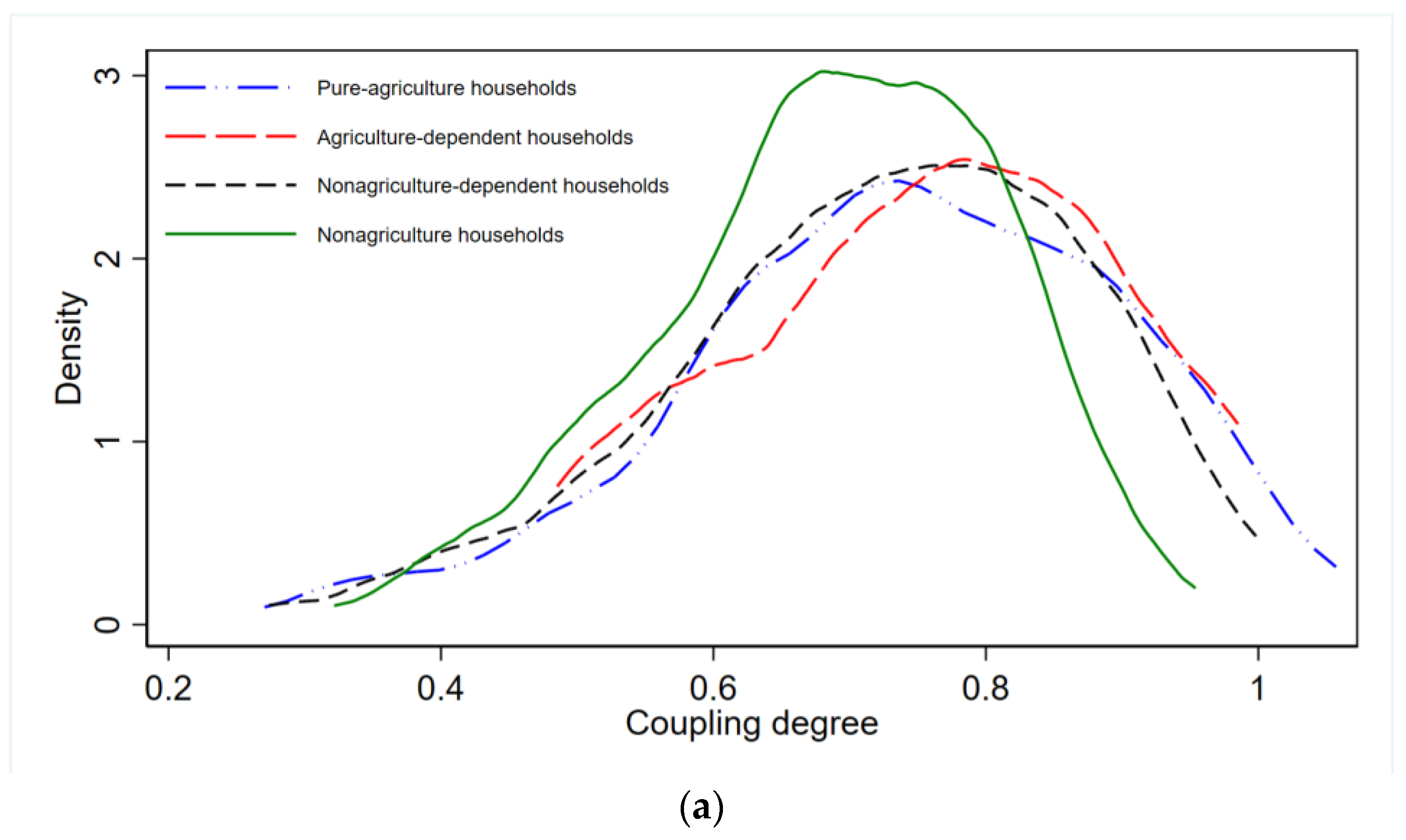
The concentration of coupling degree is different for various types of households. Among them, the difference of nonagricultural households is smaller (the concentration range is 0.566–0.802), and the difference of pure-agricultural households is larger (the concentration range is 0.404–0.903).

(2)

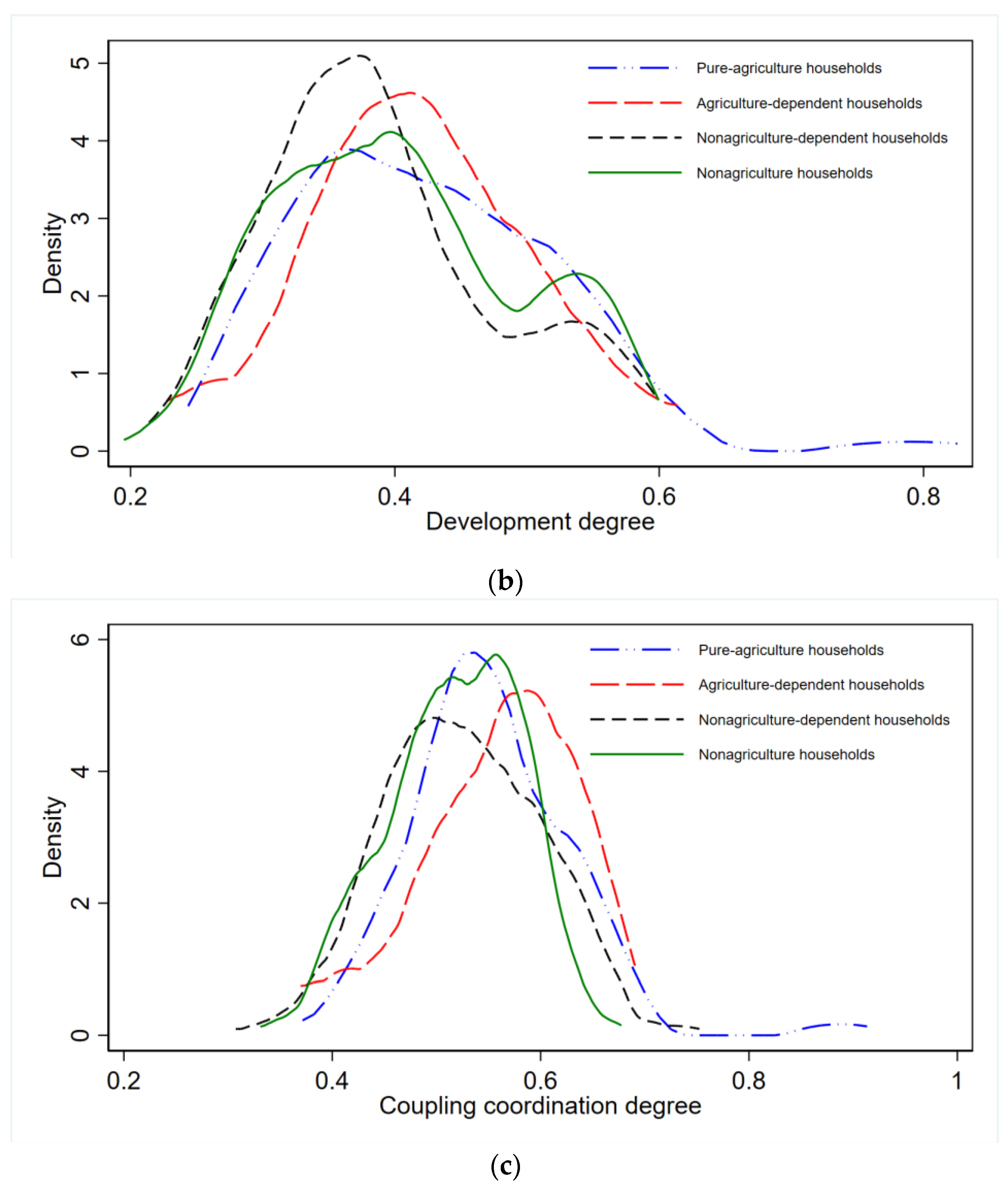
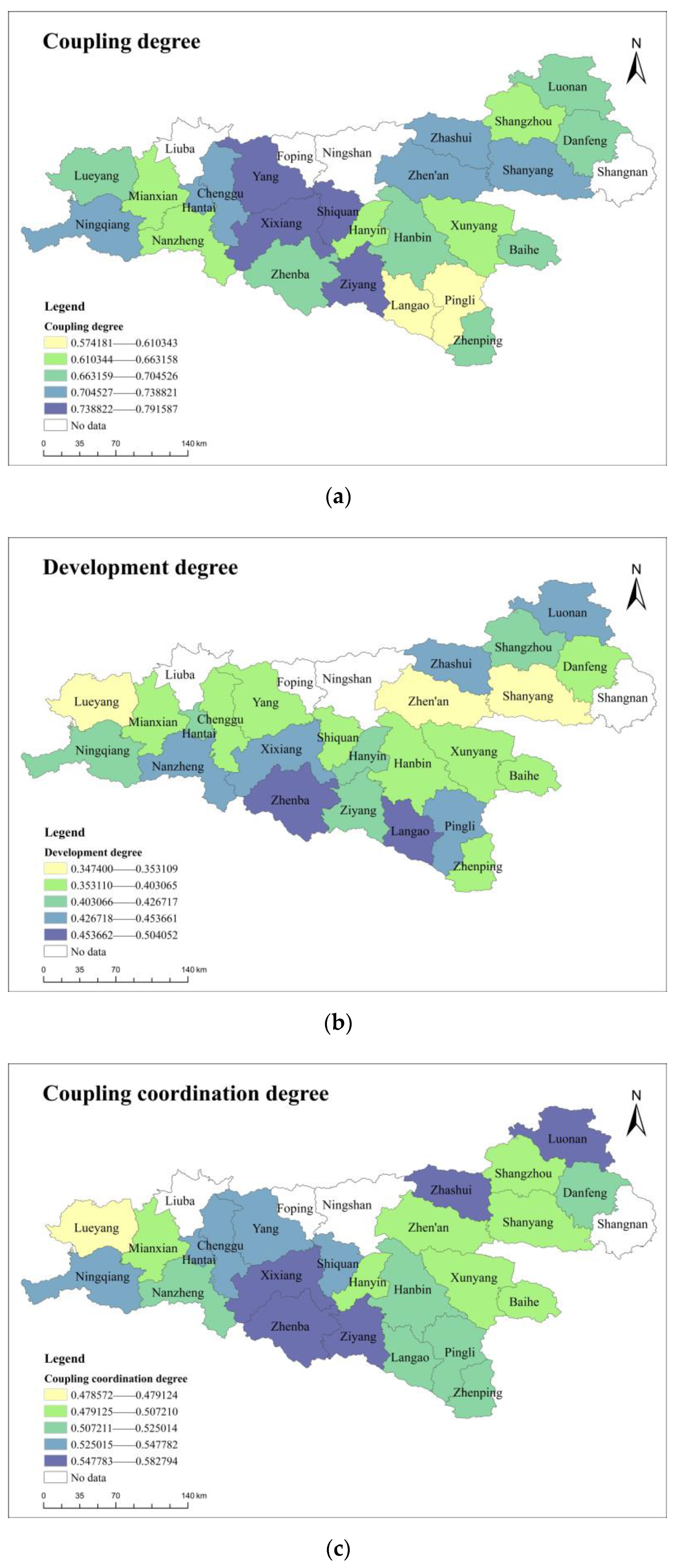
The coupling degrees of different types of households are different for various districts and counties. Comparing various types of households, the coupling degree of pure-agriculture households in Hantai district and the coupling degree of agriculture-dependent households in Ziyang county are lower. The coupling degree of pure-agricultural households and nonagriculture-dependent households in Zhenping county, the coupling degree of nonagricultural households in Luonan county and the coupling degree of pure-agricultural households in Danfeng county are lower.

(3)

The spatial distribution patterns of the coupling degree are different for various types of households. From east to west, the distribution coupling degree of nonagricultural households and agriculture-dependent households (U-shaped) is opposite to those of other types of households (inverted U-shaped). From north to south, the coupling degree of agriculture-dependent households (U-shaped) is opposite to those of other types of households (inverted U-shape).

This is mainly because the land use level has a greater impact on the coupling degree of households. The livelihood activities of pure-agriculture households, nonagriculture-dependent households and agriculture-dependent households all involve agricultural production, which result in the spatial similarity of the development pattern of coupling degree of households and the land use level. As for nonagricultural households, nonagricultural activities weaken the impact of land use, and different livelihood means differentiate household livelihood and land use and affect the households coupling degree. Driven by the land use level and livelihood efficiency, the coupling degree of households also shows a spatially differentiated development trend.

3.5.2. Spatial Differentiation of the Development Degree of Households in Different Types and Regions

According to the spatial distribution and trend of the development degree of different types of households, it can be seen that there are slight lag state and primary development state for each type of household in all districts and counties. Specifically, the development degree of each type of households has the following spatial rules.

(1)

The concentrations of development degrees are different for various types of households. Among them, the difference of nonagricultural households is smaller (concentration range is 0.300–0.489), while the difference of agricultural-dependent households is larger (concentration range is 0.261–0.551).

(2)

The development degrees of different types of households are different in various districts and counties. Compared with various types of households, the development degrees of pure-agriculture households and agriculture-dependent households in Hantai district are relatively lower. The development degrees of pure-agriculture households and nonagriculture-dependent households in Ziyang county are relatively lower. The development degrees of nonagriculture-dependent households and agriculture-dependent households in Zhenping county are relatively higher. The development degrees of pure-agriculture households and agriculture-dependent households in Luonan county and the development degree of nonagriculture households in Danfeng county are relatively lower.

(3)

The spatial distribution patterns of the development degrees are different for various types of households. From east to west, the distribution of the development degree of pure-agriculture households (U-shape”) is opposite to those of other types of households (inverted U-shaped). From north to south, the distribution of the development degree of agriculture-dependent households (inverted U-shaped) is opposite to those of other types of households (U-shaped). The development degree of nonagriculture-dependent households is characterized by being high in the north and low in the south from north to south, while the development degree of other types of households is characterized by being low in the north and high in the south.

This is because the development degree of households is mainly affected by livelihood efficiency and land use level. In the entire space, the development degree of household livelihood efficiency is significantly higher than that of the land use level, which subjects the development degree of households to more impact by the changes of livelihood efficiency and presents a similar development pattern.

3.5.3. Spatial Differentiation of the Coupling Coordination Degree of Households in Different Types and Regions

According to the spatial distribution and trend of the coupling coordination degree of different types of households, there are primary coordination state, intermediate coordination state for pure-agriculture, agriculture-dependent, and nonagriculture-dependent households in all districts and counties, but the coupling coordination degree of nonagriculture households is at the primary coordination state in all districts and counties. Specifically, the coupling coordination degree of various types of households has the following spatial patterns.

(1)

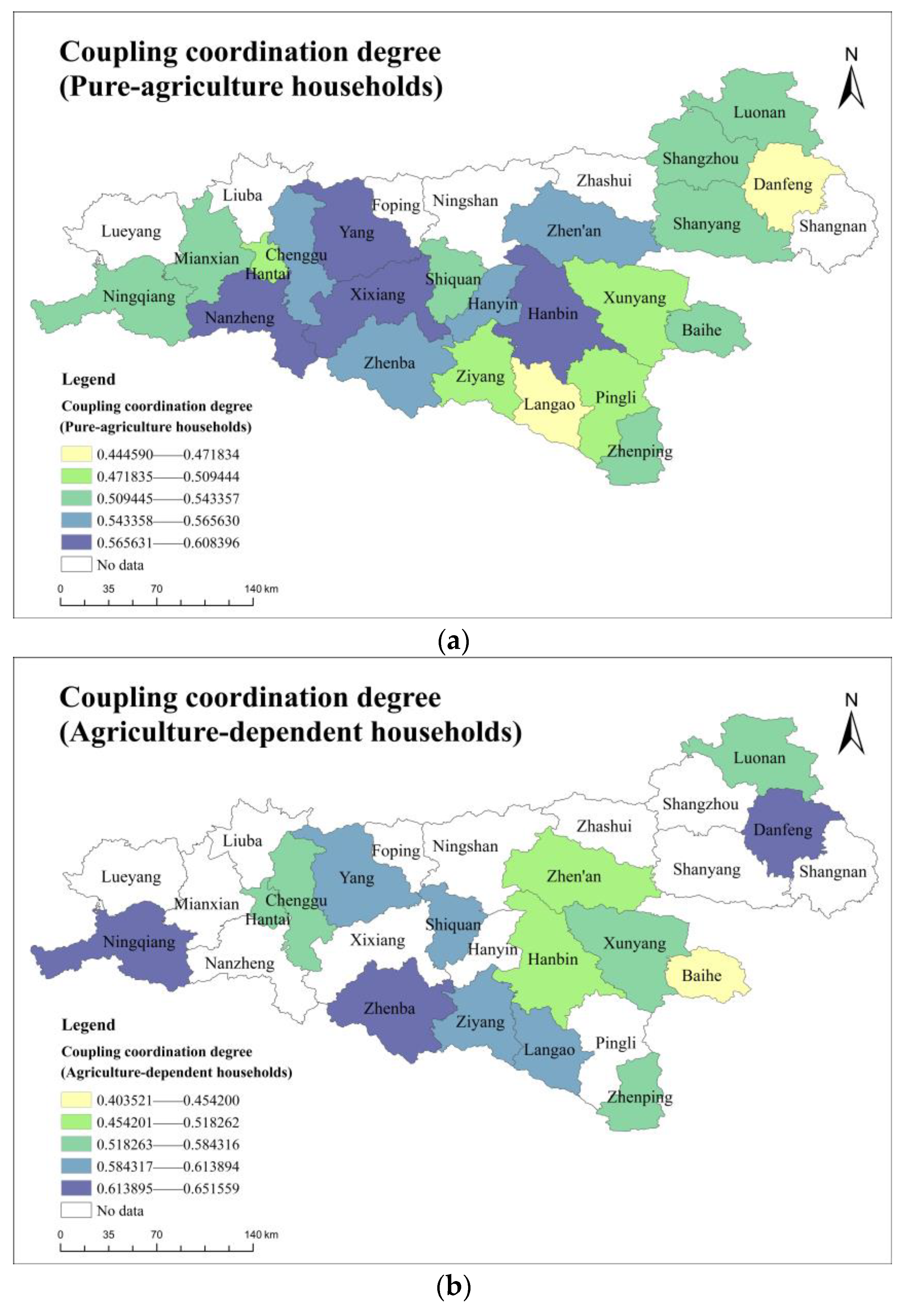
The concentrations of coupling coordination degrees are different for various types of households. Among them, the difference between nonagriculture households is smaller (the concentration range is 0.459–0.571), and the difference between agriculture-dependent households is relatively larger (the concentration range is 0.404–0.652).

(2)

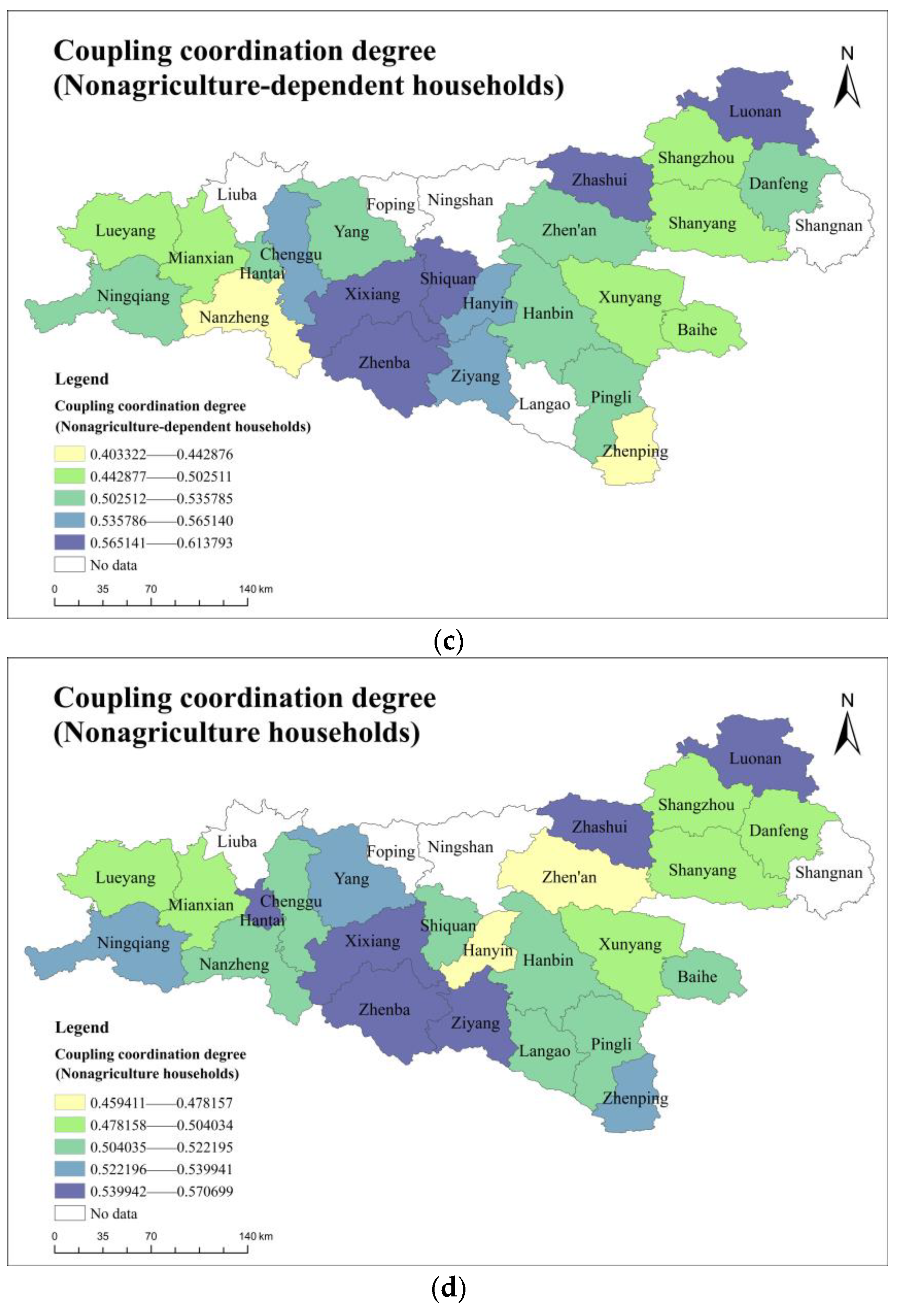
The coupling coordination degrees of different types of households are different in districts and counties. Comparing various types of households, the coupling coordination degree is lower for pure-agriculture households in Hantai district, pure-agriculture households in Ziyang county, nonagriculture-dependent households in Zhenping county, pure-agriculture and agriculture-dependent households in Luonan county and pure-agriculture and nonagriculture households in Danfeng county.

(3)

The spatial distribution patterns of coupling coordination degree are different for various types of households. From east to west, the distribution of the coupling coordination degree of agriculture-dependent households (U-shaped) is opposite to those of other types of households (inverted U-shaped), and the coupling degree of agriculture-dependent households is characterized by being high in the west and low in the east from north to south. The distribution of the coupling coordination degree of agriculture-dependent and nonagriculture households (U-shaped) is opposite to those of other types of households (inverted U-shaped). The difference of coupling coordination degree of agriculture-dependent households in south-north direction is small, and the coupling coordination degree of nonagriculture-dependent households is characterized by being high in the north and low in the south.

This is mainly because the coupling coordination degree not only reflects the relationship between household livelihood efficiency and land use level, but also reflects the degree of benign coupling between them. Land use is the basis and primary condition for the mutual influence of household livelihoods and land use, and livelihood efficiency reflects the benign influence of household livelihoods and land use to a certain extent. Under the combined effect of land use level (primary) and livelihood efficiency (secondary), the coupling coordination degree of different types of households shows different development trends. For example, under the influence of land use level, the coupling coordination degree of nonagriculture-dependent households shows a trend of being high in the middle and low around in space. However, affected by the livelihood efficiency, the coupling coordination degree of nonagriculture-dependent households is characterized by being high in the north and low in the south.

4. Discussion

4.1. Optimization Measures

With the development of society and economy, the household livelihood system and land system in mountainous areas gradually show a more resistant and restrained state, which not only causes a waste of livelihood resources but also threatens the country’s farmland security and food security. To solve this problem, it is necessary to guide the coordinated development of the household livelihood system and land system and maximize the livelihood efficiency while improving the households’ land use level. To this end, improvements can be made from the perspectives of the types of households and geographical space, among other things. The following are some suggestions.

(1)

Develop differentiated livelihood optimization plans based on different types of households. ① Pure-agriculture households can improve their coupling coordination by improving agricultural infrastructure, adjusting land planting structure (food crops, cash crops.), expanding land planting scale, optimizing agricultural production methods, adjusting agricultural production structure (planting, breeding). ② For agriculture-dependent households, they can optimize their agricultural production structure to improve their livelihood efficiency and land use level. On the other hand, they can broaden the scope of their nonagricultural activities, enrich the types of nonagricultural activities, and choose more suitable and efficient nonagricultural activities to coordinate the relationship between agricultural activities and nonagricultural activities and improve the livelihood efficiency. ③ Nonagriculture-dependent households can flexibly adjust their land use methods according to their working hours and work content to maximize the use of livelihood resources. For example, they can optimize the planting structure and breeding structure by planting mulberries, walnut trees, and wild pepper trees, among other things, to improve their livelihood efficiency. ④ Nonagriculture households can adjust the land use form according to their working location and work content. For example, land can be transferred and contracted, and mulberries, walnut trees, traditional Chinese medicine herbs, fruit trees and other crops with less input can be planted. In addition, they can join rural production cooperatives and use land resource to obtain a certain income dividend.

(2)

Develop appropriate livelihood development strategies according to different geographical spaces. On the one hand, it is also advisable to develop the livelihood development strategies according to the regional livelihood efficiency and land use level. ① In areas where the livelihood efficiency and land use level are generally low, such as Lueyang county and Shanyang county, it is advisable to help households choose production methods with higher livelihood efficiency, more reasonable land use structure, and higher land use efficiency, to improve the households’ livelihood efficiency, land use level and the coupling coordination level. ② In areas with lower livelihood efficiency and higher land use levels, such as Shiquan county and Yang county, restrictions on land resources make it difficult for households to improve their livelihood efficiency. In this case, households need to develop appropriate nonagricultural activities to supplement the agricultural production to improve livelihood efficiency. ③ In areas with high livelihood efficiency and low land use levels, such as Langao county and Pingli county, the low land use level weakens the coupling coordination relationship between households’ livelihood efficiency and land use. In the future, it is necessary to innovate livelihood methods and land use methods, and improve the land use level on the basis of ensuring the livelihood efficiency. ④ In areas where the livelihood efficiency and land use level are generally high, such as Luonan county and Zhenba County, the coupling coordination degree of household livelihood efficiency and land use can be continuously improved by improving the infrastructure, optimizing the ecological environment, and increasing employment opportunities. And the coupling coordination degree cannot focus on a single aspect of livelihood efficiency or land use level. On the other hand, it will be effective to develop corresponding plans according to regional characteristics. ① In areas with higher terrain, it can not only guide households to plant or breed agricultural products with higher added value according to local characteristics, but also promote the development of production and life models such as building parks on the mountains, building communities under the mountains, and turning households to workers. ② In areas with lower terrain, households can improve their productivity through scale, informatization and mechanization, and they can also use diversified livelihood means to increase income. ③ In areas with a high level of economic development, the income of households can be increased through various production modes such as specialization in production, concurrent employment, and large-scale production. ④ In areas with a low level of economic development, the income of households can be increased by means of labor transfer, and the living standards of households can be improved by attracting investment and improving infrastructure.

(3)

Comprehensively improve the livelihood ability and livelihood conditions of households according to the types of households and the characteristics of the geographical space. In order to promote the coordinated and sustainable development of household livelihood efficiency and land use, not only should the households’ own livelihoods be taken into account, but also the external livelihood environment needs to optimized, so as to achieve the high-quality development of households through the “internal and external integration” method. Specifically, improvements can be made of the following aspects: ① Improve the utilization quality and level of land resources. On the one hand, the quality of land use can be improved by implementing a “slope-to-terracing” project, constructing irrigation facilities, transforming farmland, water-electricity-road networks, and improving rural development supporting facilities. On the other hand, land use level can be improved from the perspectives of the market, system, and types of households. For example, the government can guide households to plant crops with higher efficiency and less time and energy, and at the same time, the government can encourage households to work out by land transfer, land lease, and land shares. ② Encourage households to change production methods. When choosing a mode of production, households should comprehensively consider their own family conditions and the local environment. For example, households with less land resources can switch to part-time or full-time nonagricultural activities to increase their income levels, households with more land resources can improve their livelihood efficiency through large-scale production and mechanized production, while households with medium-level land resources can engage in agricultural and nonagricultural production at the same time. Households with formal nonagricultural jobs can engage in agricultural production during holidays and after work, and households without formal nonagricultural jobs can go out to work during the slack time or engage in part-time jobs in the surrounding towns. ③ Promote the development of characteristic industries. It is necessary to promote the development of characteristic industries and realize the commercialization of agriculture by households based on the advantages of regional resources and environment. For example, households can be encouraged to plant special cash crops such as tea, traditional Chinese medicine herbs, peppers, konjac, and walnut trees. Households can be guided to increase their income by adopting methods such as “rice-fish symbiosis”, “rice-shrimp symbiosis” and “under-forest economy”. Households can be encouraged to rely on regional tourism development plan to engage in farmhouses, picking gardens, stay home on farm, handicrafts, characteristic agricultural products, etc. ④ Improve the level of education and medical care. The education level and health status of the households themselves are the basis for carrying out livelihood activities. To this end, the ability of households can be guaranteed and improved by carrying out skill training, regular physical examinations, delivering market information, and organizing medical activities in the countryside.

In general, in order to improve household livelihood capacity and livelihood quality and realize regional coordinated and sustainable development, households and the government need to participate together. For households, it is necessary to stimulate their initiative, enthusiasm and creativity, and encourage them to improve their livelihood quality by improving production technology, adjusting production strategies and optimizing the allocation of livelihood resources. For the government, it needs to guide and support households. On the one hand, government departments need to constantly improve the “hard environment” in rural areas. Water conservancy, electric power, roads, networks and other infrastructure are the basis for households and rural development. Government departments should not only actively improve the infrastructure of each region, but also invest in the construction of relevant facilities according to the characteristics of different regions to promote regional development. On the other hand, government departments need to promote and improve the “soft environment” in rural areas. Creating a good medical and educational environment can not only improve the comprehensive quality of households, but also provide guarantee for the development of households.

4.2. Limitation

There are still some limitations in this study. (1) This study only calculates the livelihood efficiency, land use level, coupling degree, development degree and coupling coordination degree of households, and analyzes the differences between households of different types and regions, but there is no in-depth analysis of the reasons behind the differences, and it does not explore the relevant factors through quantitative analysis. Therefore, in the future research, it is necessary to further verify the viewpoint of this study, design the index system from the perspectives of geographical environment, regional development level, infrastructure level, livelihood risk and livelihood capital, and further analyze the key factors affecting the coupling coordination relationship between household livelihood efficiency and land use. (2) When analyzing the spatial characteristics of households, this study mainly used ArcGIS software to visually display the relevant results from a spatial perspective, and used the trend surface analysis tool to explore the spatial differentiation trend of the coupling coordination relationship between household livelihood efficiency and land use. However, in general research, exploratory spatial data analysis (ESDA) is often used to explore the differentiation characteristics at the spatial level. In the future, a variety of methods should be used to supplement and improve the relevant research content.

5. Conclusions

The coupling coordination relationship between household livelihood efficiency and land use refers to a state in which the livelihood system and the land system interact to optimize the overall situation and develop jointly driven by natural, economic, social, location, and market factors. From the perspective of households themselves and the external spatial environment, an in-depth analysis of the coupling coordination relationship between household livelihood efficiency and land use can provide reference for the comprehensive, coordinated and sustainable development for households in the area studied and similar regions. Through the analysis of the relevant results, the following conclusions can be drawn.

(1)

The overall livelihood efficiency of households in Qinba is at a medium level. The overall land use level is quite different and low, the coupling degree is at the intermediate coupling state, the development degree is at the primary development state, and the coupling coordination degree is at the primary coordination state. In order to promote the sustainable, coordinated, and high-quality development of household livelihood efficiency and land use, we should not only focus on household land use, but also improve household livelihood efficiency through a variety of methods, such as optimizing livelihood structure and improving production technology.

(2)

From the perspective of the types of households, with the increase of nonagricultural degree, the coupling coordination degree of households increases first, and then decreases. Under the influence of household livelihood methods and land use methods, there are certain differences in the coupling coordination relationship between various types of household livelihood efficiency and land use. Among them, pure-agriculture households have the highest development degree; agriculture-dependent households have the highest land use level, coupling degree, and coupling coordination degree; nonagriculture-dependent households have the lowest development degree and livelihood efficiency; nonagriculture households have the highest livelihood efficiency, lowest land use level, coupling degree, and coupling coordination degree.

(3)

From the perspective of spatial distribution pattern, the coupling coordination degree for households east-to-west is “sagging”, while south-to-north diagram is “hogging”. Under the influence of topography, social and economic development level, geographic location and infrastructure, the coupling coordination relationship between household livelihood efficiency and land use are different in regional space. Compared with the central region, the livelihood efficiency, land use level, coupling degree, development degree, and coupling coordination degree of households in the western and eastern regions are relatively lower; the livelihood efficiency, development degree, and coupling coordination degree of households in the northern and southern regions are relatively higher and their land use level and coupling degree are lower.

(4)

From the perspective of the households themselves and the external spatial environment, the distribution of the coupling coordination degree for agriculture-dependent households east-to-west (the “sagging” diagram) is opposite to the other types of households. By analogy, the distribution of the coupling coordination degree for nonagriculture and agriculture-dependent households north-to-south (the “hogging” diagram) is opposite to the other types of households. Under the combined influence of household livelihood ability and the external environment, the coupling coordination relationship between different types of household livelihood efficiency and land use are different in space. For example, the livelihood efficiency and development degree of pure-agriculture households are spatially characterized by being low in the middle and high around, and the land use level, coupling degree, and coupling coordination degree are spatially characterized by being high in the middle and low around the sides; the livelihood efficiency and development degree of agriculture-dependent households are spatially characterized by being high in the middle and low around, and the land use level, coupling degree, and coupling coordination degree are spatially characterized by being low in the middle and high around.

The coupling coordination relationship between household livelihood efficiency and land use is affected by regional development level, resource, geographic location, infrastructure level and many other factors. The household livelihood efficiency, the interaction among various elements in the land use system and the feedback mechanism should be deeply analyzed in the future to reveal the coupling coordination mechanism between household livelihood efficiency and land use. In addition, different intervention optimization plans can be designed for different types of households in different regions, and an integrated livelihood efficiency and land use coupling coordination composite system may be constructed. The optimization schemes may be simulated with the help of the composite system, in order to provide a scientific, reasonable and operable reference for establishing a diversified and multi classification comprehensive optimization system of coupling coordination of livelihood efficiency and land use.

References

1. Wu, C.J. Theoretical research and regulation of the regional system of human-land relationship. J. Yunan Norm. Univ. (Humanit. Soc. Sci. Ed.) 2008, 211, 1–3. [Google Scholar]
2. Zheng, X.Y.; Liu, Y.S. Connotation, formation mechanism and regulation strategy of “rural disease” in the new epoch in China. Hum. Geogr. 2018, 33, 100–106. [Google Scholar]
3. Li, X.Y.; Yang, Y.; Liu, Y.; Chen, Y.Y.; Xia, S.Y. The Systematic Structure and Trend Simulation of China’s Man-land Relationship Until 2050. Sci. Geogr. Sin. 2021, 41, 187–197. [Google Scholar]
4. Su, F.; Xu, Z.M.; Shang, H.Y. An overview of sustainable livelihoods approach. Adv. Earth Sci. 2009, 24, 61–69. [Google Scholar]
5. Su, F.; Pu, X.D.; Xu, Z.M.; Wang, L.A. Analysis about the relationship between livelihood capital and livelihood strategies: Take Ganzhou in Zhangye city as an example. China Popul. Resour. Environ. 2009, 19, 119–125. [Google Scholar]
6. Xu, H.S.; Yue, Z. Livelihood strategies of livelihood capital, livelihood risks and farmers. Probl. Agric. Econ. 2012, 33, 100–105. [Google Scholar]
7. Guo, S.Q.; Zhang, J.W. Analysis on farmers’ livelihood capital vulnerability. Econ. Surv. 2013, 3, 26–30. [Google Scholar]
8. Guo, R.W.; Liu, S.Q.; Chen, G.J.; Xie, F.T.; Yang, X.J.; Liang, L. Research progress and tendency of sustainable livelihoods for peasant household in China. Prog. Geogr. 2013, 32, 657–670. [Google Scholar]
9. Luo, C.; Wang, Y. Getting rid of rural poverty: Explanation and policy choice of sustainable livelihood analysis framework. J. Humanit. 2020, 288, 113–120. [Google Scholar]
10. Hu, L.; Lu, Q. The effect of livelihood capability on farmers’ persistent poverty threshold. J. Huazhong Agric. Univ. (Soc. Sci. Ed.) 2019, 143, 78–87, 169–170. [Google Scholar]
11. Tan, S.H.; Qu, F.T.; Huang, X.J. Difference of farm households’ land use decision-making and land conservation policies under market economy. J. Nanjing Agric. Univ. 2001, 24, 110–114. [Google Scholar]
12. Yan, J.Z.; Zhuo, R.G.; Xie, D.T.; Zhang, Y.L. Land use characters of farmers of different livelihood strategies: Cases in three gorges reservoir area. Acta Geogr. Sin. 2010, 65, 1401–1410. [Google Scholar]
13. Yang, X.Y.; Zhou, H.; Liu, X.H. Analysis on land use efficiency and its driving factors of different farming households types in mountainous areas—A case study of 18 sample villages in Wuling mountainous area. Chin. J. Agric. Resour. Reg. Plan. 2020, 41, 122–130. [Google Scholar]
14. Zu, H.Q.; Zhao, C.W. Spatial differentiation and influencing factors of cultivated land use intensity in Karst trough area: A case study of the Langxi Valley in Guizhou Province, China. Mt. Res. 2021, 39, 415–428. [Google Scholar]
15. Liao, L.W.; Gao, X.L.; Long, H.L.; Tang, L.S.; Chen, K.Q.; Ma, E.P. A comparative study of farmland use morphology in plain and mountainous areas based on farmers’ land use efficiency. Acta Geogr. Sin. 2021, 76, 471–486. [Google Scholar]
16. Zhu, C.M.; Huang, Y.D.; Wu, J.; Peng, Q. Spatial disparity of cultivated land intensive utilization and its driving forces based on different types of geomorphology—A case study of Jiangxi Province. J. Mt. Sci. 2012, 30, 156–164. [Google Scholar]
17. Liu, H.B.; Wang, Q.B.; Bian, Z.X.; Yu, G.F.; Sun, Y. Studying the characteristics and its influencing factors of the farmer land use behavior in the process of industrialization and urbanization: A case study in Sujiatun District of Shenyang City, Liaoning Province. China Popul. Resour. Environ. 2012, 22, 111–117. [Google Scholar]
18. Wang, X.Y.; Yan, J.Z. Cultivated land use intensity and its influencing factors of households of different livelihood strategies: A case study of 12 typical villages in Chongqing Municipality. Geogr. Res. 2015, 34, 895–908. [Google Scholar]
19. Liu, T.; Qu, F.T.; Jin, J.; Shi, X.P. Impact of land fragmentation and land transfer on farmer’s land use efficiency. Resour. Sci. 2008, 30, 1511–1516. [Google Scholar]
20. Jampel, C. Cattle-based livelihoods, changes in the taskscape, and human–bear conflict in the Ecuadorian Andes. Geoforum 2016, 69, 84–93. [Google Scholar] [CrossRef]
21. Zhao, X.Y. Sustainable livelihoods research from the perspective of geography: The present status, questions and priority areas. Geogr. Res. 2017, 36, 1859–1872. [Google Scholar]
22. Zhao, X.Y.; Li, W. Review of Gannan research in Chinese geography. Geogr. Res. 2019, 38, 743–759. [Google Scholar]
23. Yang, L.; Liu, M.C.; Yan, Q.W.; He, S.Y.; Jiao, W.J. Review of eco-environmental effect of farmers’ livelihood strategy transformation. Acta Ecol. Sin. 2019, 39, 8172–8182. [Google Scholar]
24. Wang, C.C.; Yang, Y.S. An overview of farmers’ livelihood strategy change and its effect on land use/cover change in developing countries. Prog. Geogr. 2012, 31, 792–798. [Google Scholar]
25. Duan, W.; Ren, Y.M.; Feng, J.; Wen, Y.L. Study on natural resource dependence based on livelihood assets: Examples from nature reserves in Hubei Province. Issues Agric. Econ. 2015, 36, 74–82, 112. [Google Scholar]
26. Edward, R.C.; Brent, M. The co-production of land use and livelihoods change: Implications for development interventions. Geoforum 2009, 40, 568–579. [Google Scholar]
27. Hu, R.; Xie, D.T.; Qiu, D.C.; Wang, X.Y. Review of land use and rural livelihood at home and abroad. Areal Res. Dev. 2016, 35, 162–167. [Google Scholar]
28. Albinus, M.P.M.; Joy, O.; Yazidhi, B. Effects of land use practices on livelihoods in the transboundary sub-catchments of the Lake Victoria Basin. Afr. J. Environ. Sci. Technol. 2008, 2, 309–317. [Google Scholar]
29. Liang, L.T.; Qu, F.T.; Zhu, P.X.; Ma, K. Analysis of land use behavior and efficiency of different farm household types. Resour. Sci. 2008, 30, 1525–1532. [Google Scholar]
30. Ding, S.J.; Zhang, Y.Y.; Ma, Z.X. Research on changes of livelihood capabilities of rural households encountered by land acquisition: Based on improvement of sustainable livelihood approach. Issues Agric. Econ. 2016, 37, 25–34, 110–111. [Google Scholar]
31. Liu, Y.M.; Li, S.Z. Study on the development stages of household livelihood diversification: Based on the dimensions of vulnerability and adaptability. China Popul. Resour. Environ. 2017, 27, 147–156. [Google Scholar]
32. Ma, C.; Liu, L.M.; Yuan, C.C.; Ren, G.P. Evaluation of cultivated land use intensity of different types of rural household livelihood strategies in rapid urbanization area: A case of Qingpu District in Shanghai City. China Land Sci. 2017, 31, 69–78. [Google Scholar]
33. Shaanxi Bureau of Statistics. Shaanxi Statistical Yearbook; China Statistic Press: Beijing, China, 2020. [Google Scholar]
34. Liu, Q.; Chen, J.; Wu, K.S.; Yang, X.J. Multidimensional poverty measurement and its impact mechanism on households in the Qinling-Daba Mountains poverty area: A case of Shangluo city. Prog. Geogr. 2020, 39, 996–1012. [Google Scholar] [CrossRef]
35. He, Z.W. An analysis on the causes of farmers’ persistent poverty in Qinba mountainous area of Southern Shaanxi from the perspective of livelihood ability. J. Xi’an Univ. Arts Sci. (Soc. Sci. Ed.) 2020, 23, 103–106. [Google Scholar]
36. Li, J. Study on the Spatial Differences and Influencing Factors of Poor Rural Households’ Livelihood Based on the Expanded Sustainbale Livelihood Framework: A Case Study of Shizhu County, Chongqing. Ph.D. Thesis, Southwest University, Chongqing, China, 2018. [Google Scholar]
37. Wu, Y. Poor mountain farmers livelihood capital impact on livelihoods strategy research: Based on the survey data Pingwu and Nanjiang County of Sichuan Province. Issues Agric. Econ. 2016, 37, 88–94, 112. [Google Scholar]
38. Wu, L.; Jin, L.S. Study on influential factors of peasant households’ livelihood capital under the policy of eco-compensation poverty alleviation. J. Huazhong Agric. Univ. (Soc. Sci. Ed.) 2018, 6, 55–61, 153–154. [Google Scholar]
39. Su, F.; Ma, N.N.; Song, N.N.; Yin, Y.J.; Kan, L.N. Analysis on the difference of the implementation effect of different poverty alleviation measures—Based on the framework of sustainable livelihood approach. China Soft Sci. 2020, 1, 59–71. [Google Scholar]
40. Liu, X.B.; Wang, Y.K.; Li, M.; Liu, Q.; Zhang, Y.X.; Zhu, Y.Y. Analysis on coupling coordination degree between livelihood strategy for peasant households and “production, living and ecological” functions of lands in typical mountainous areas, China. Mt. Res. 2020, 38, 596–607. [Google Scholar]
41. Zhang, Y.P.; Halike, W.; Dang, J.H.; Deng, B.S.; Wang, R. Coupled coordination degree of tourism-economy-ecological system in Turpan area. Hum. Geogr. 2014, 29, 140–145. [Google Scholar]
42. Zhang, L.L.; Zheng, X.Q.; Meng, C.; Zhang, P.T. Spatio-temporal difference of coupling coordination degree of land use functions in Hunan province. China Land Sci. 2019, 33, 85–94. [Google Scholar]
43. Xu, S.; Hu, Y.C. Coupling coordination analysis of capital and livelihood stability of farmers—A case study of the resettlement area of Jinqiao village in Guangxi. Econ. Geogr. 2018, 38, 142–148, 164. [Google Scholar]
44. Chen, Y.; Tian, W.T.; Ma, W.B. The coupled relationship and spatial differences between population urbanization and land urbanization: A case study of the central plains urban agglomeration. Ecol. Econ. 2019, 35, 104–110. [Google Scholar]
45. Liu, C.J.; Zhou, J.P.; Jiang, J.H.; Wang, Z.Y. Pattern and driving force of regional innovation and regional financial coupling coordination in the Yangtze River economic belt. Econ. Geogr. 2019, 39, 94–103. [Google Scholar]
46. Li, E.L.; Cui, Z.Z. Coupling coordination between China’s regional innovation capability and economic development. Sci. Geogr. Sin. 2018, 38, 1412–1421. [Google Scholar]
47. Kuang, B.; Lu, X.H.; Zhou, M. Dynamic evolution of urban land economic density distribution in China. China Land Sci. 2016, 30, 47–54. [Google Scholar]
48. Li, J.; Hu, B.X.; Kuang, B.; Chen, D.L. Measuring of urban land use efficiency and its dynamic development in China. Econ. Geogr. 2017, 37, 162–167. [Google Scholar]
49. Li, Q.; Wang, S.J.; Mei, L. The spatial characteristics and mechanism of supermarkets in central district of Changchun, China. Sci. Geogr. Sin. 2013, 33, 553–561. [Google Scholar]
50. Xu, W.X.; Zhang, L.Y.; Liu, C.J.; Yang, L.; Huang, M.J. The coupling coordination of urban function and regional innovation: A case study of 107 cities in the Yangtze River economic belt. Sci. Geogr. Sin. 2017, 37, 1659–1667. [Google Scholar]
51. Xu, D.D.; Zhang, J.F.; Liu, S.Q.; Xie, F.T.; Cao, M.T.; Wang, X.L.; Liu, E.L. An analysis of the relationship between livelihood capital and livelihood strategies of the typical mountainous settlements in southwestern China. J. Southwest Univ. (Nat. Sci.) 2015, 37, 118–126. [Google Scholar]
52. Zhao, W.J.; Yang, S.L.; Wang, X. The relationship between livelihood capital and livelihood strategy based on logistic regression model in Xinping County of Yuanjiang dry-hot valley. Resour. Sci. 2016, 38, 136–143. [Google Scholar]
Figure 1. Location of administrative divisions of three cities in southern Shaanxi.
Land 10 01115 g001
Figure 2. Kernel density estimation diagram of the coupling coordination relationship between livelihood efficiency and land use of different types of households. Coupling degree (a), development degree (b), coupling coordination degree (c).
Land 10 01115 g002aLand 10 01115 g002b
Figure 3. Spatial distribution of the coupling coordination relationship between household livelihood efficiency and land use in different regions (districts and counties). Coupling degree (a), development degree (b), coupling coordination degree (c).
Land 10 01115 g003
Figure 4. Trend surface diagram of the coupling coordination relationship between household livelihood efficiency and land use in different regions (districts and counties). Coupling degree (a), development degree (b), coupling coordination degree (c).
Land 10 01115 g004aLand 10 01115 g004b
Figure 5. The spatial distribution of coupling coordination degrees of different types of households. Coupling coordination degree (pure-agriculture households) (a), coupling coordination degree (agriculture-dependent households) (b), coupling coordination degree (nonagriculture-dependent households) (c), coupling coordination degree (nonagriculture households) (d).
Land 10 01115 g005aLand 10 01115 g005b