
Spatially Explicit Fuzzy Cognitive Mapping for Participatory Modeling of Stormwater Management

 ,
,  , , and
Abstract
:1. Introduction
2. Methods
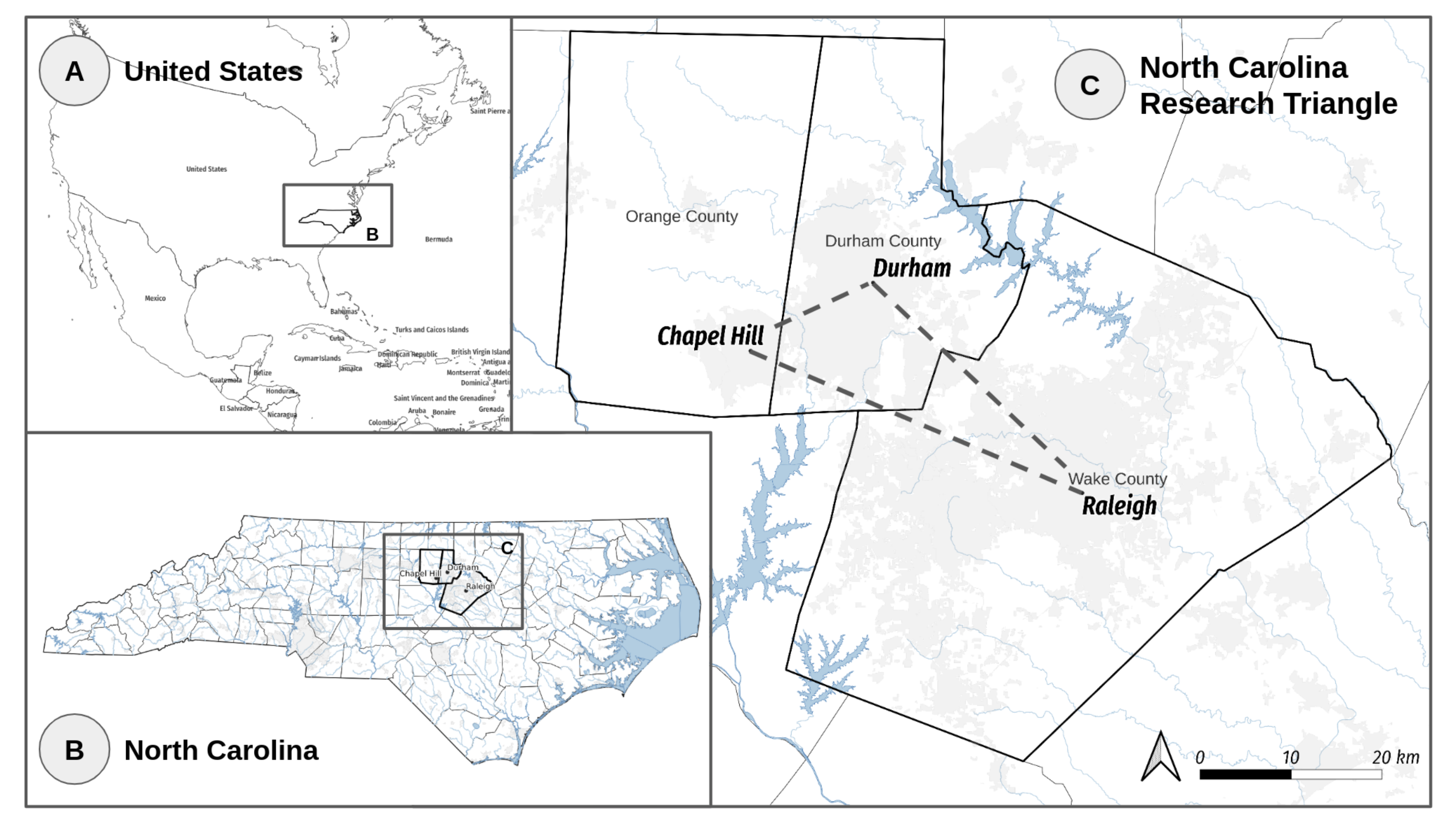
2.1. Study System
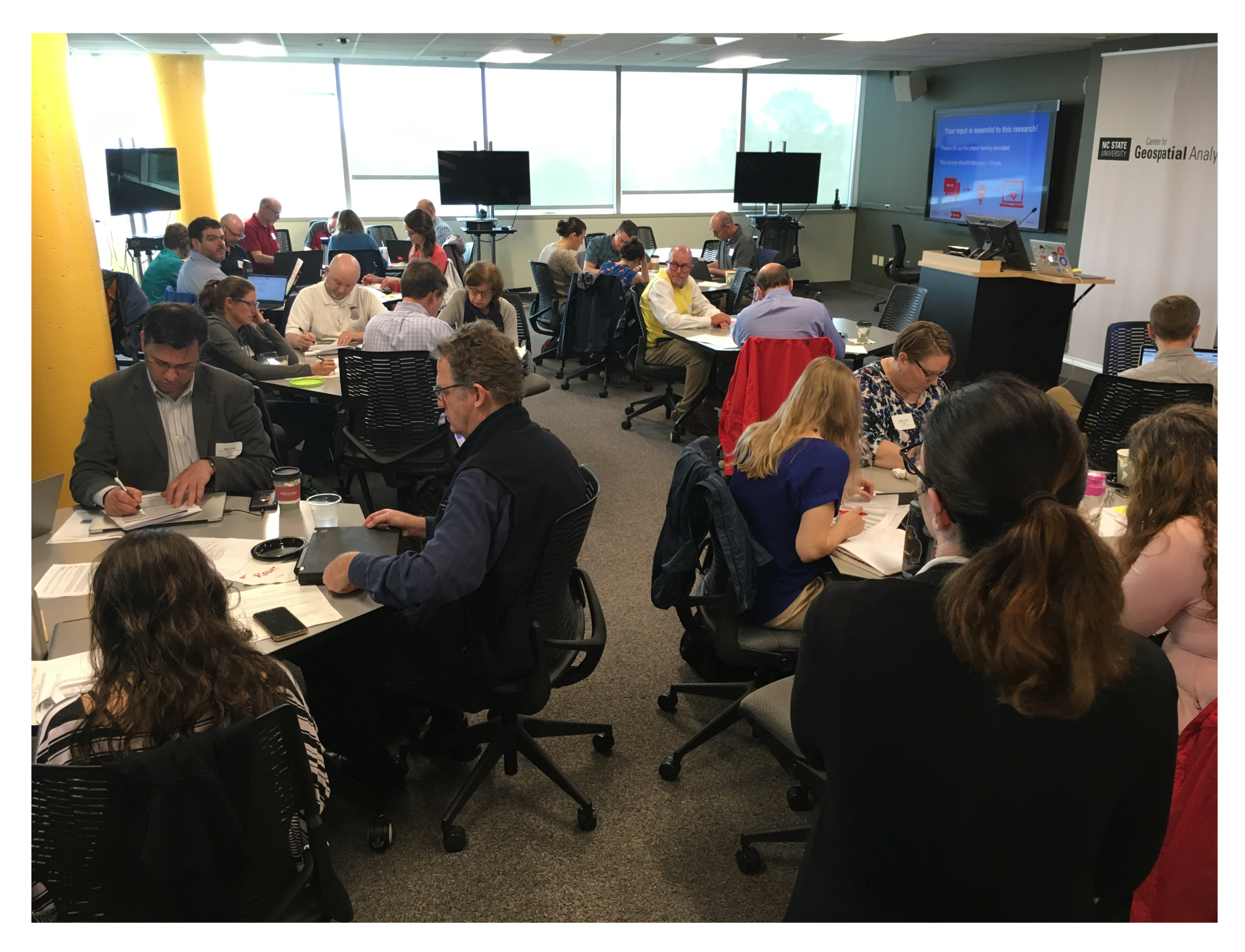
2.2. Participatory Workshops
2.3. Modeling Local Knowledge with Fuzzy Cognitive Maps
“When I mention stormwater management in the Triangle what variables/things come to mind? How do these things affect each other?”
2.3.1. Analysis of Stakeholder Groups’ FCMs
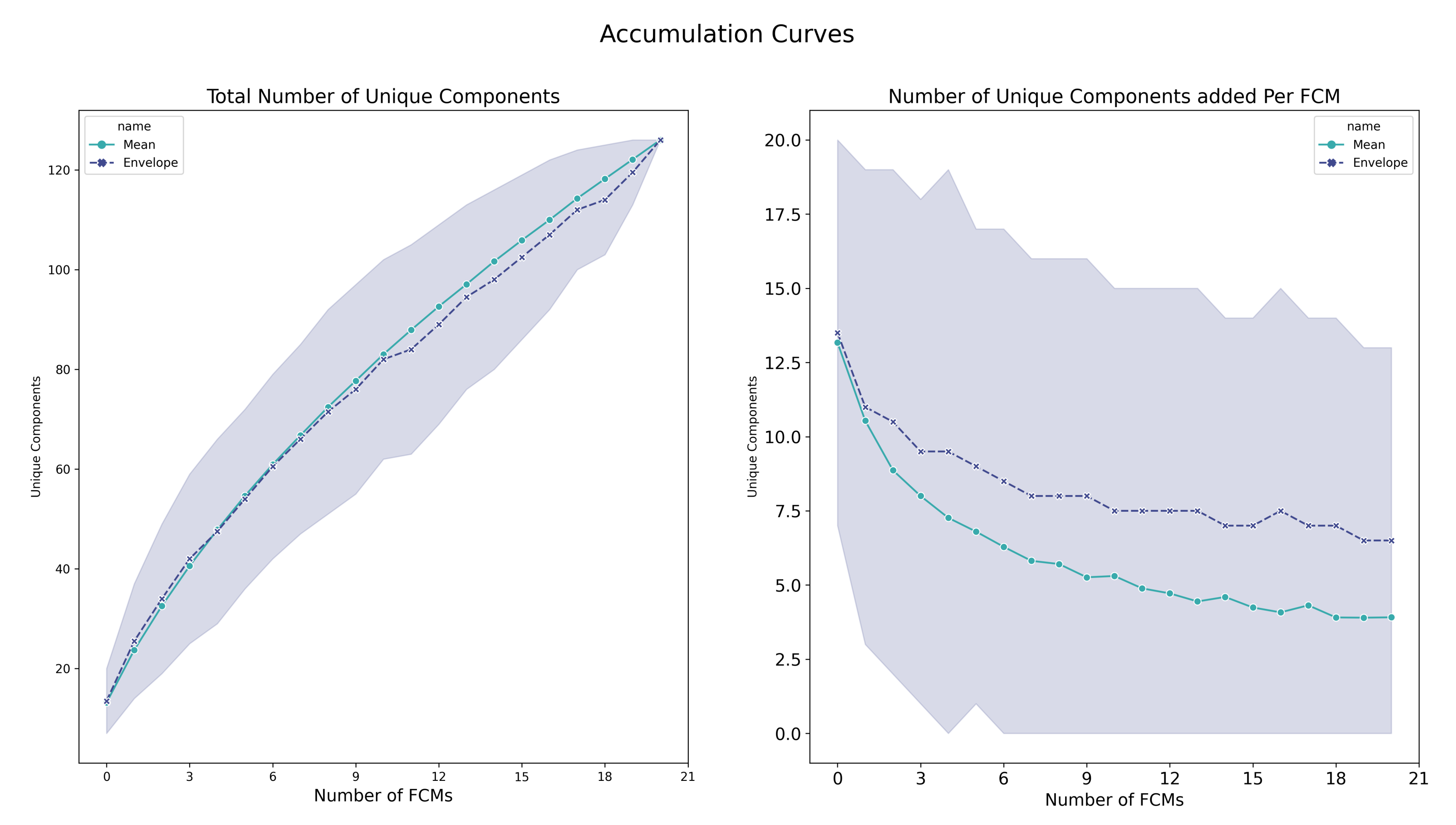
2.3.2. Model Aggregation and Evaluation of Scenarios
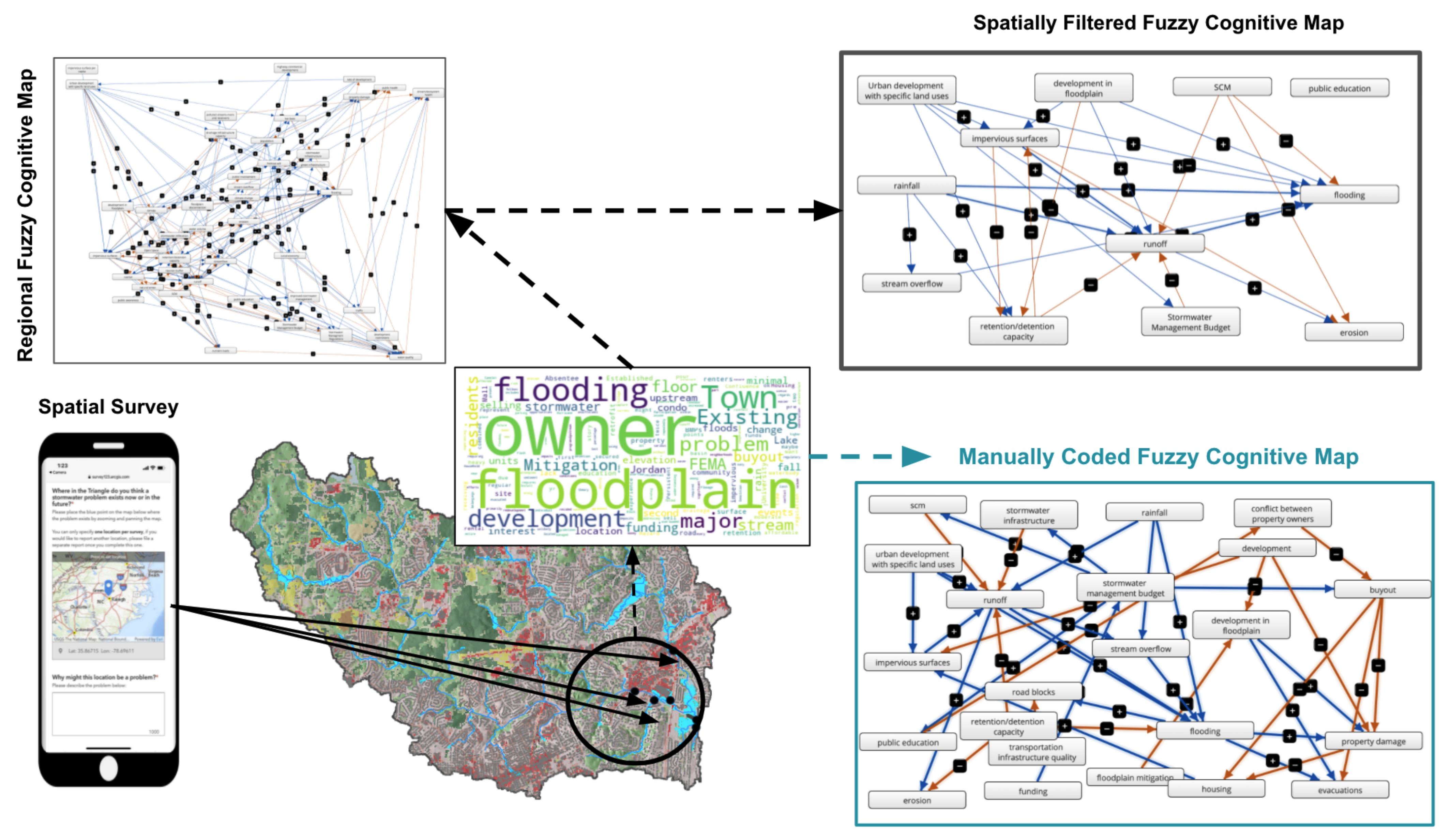
2.4. A Spatial Survey to Identify “Wicked” Stormwater Problems
- Where are some stormwater problems that currently exist in the Triangle, NC? What about in the near future?
- What are some barriers that are preventing or may happen to prevent these problems from being managed?
- What kind of actions need to be taken to resolve these problems?
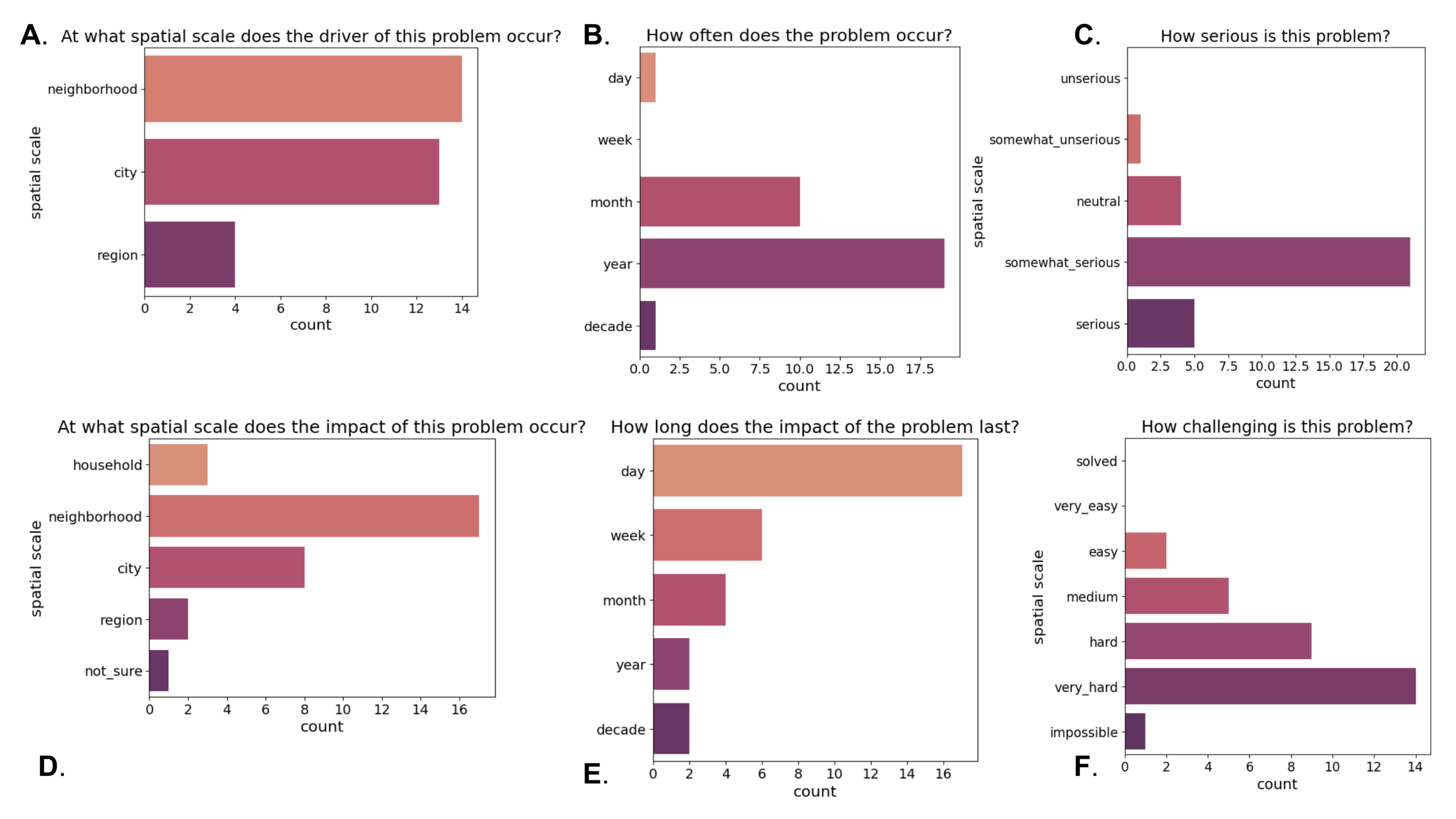
- At what spatial scale does the driver of this problem occur?
- At what spatial scale does the impact of this problem occur?
- How often does the problem occur?
- How long does the impact of the problem last?
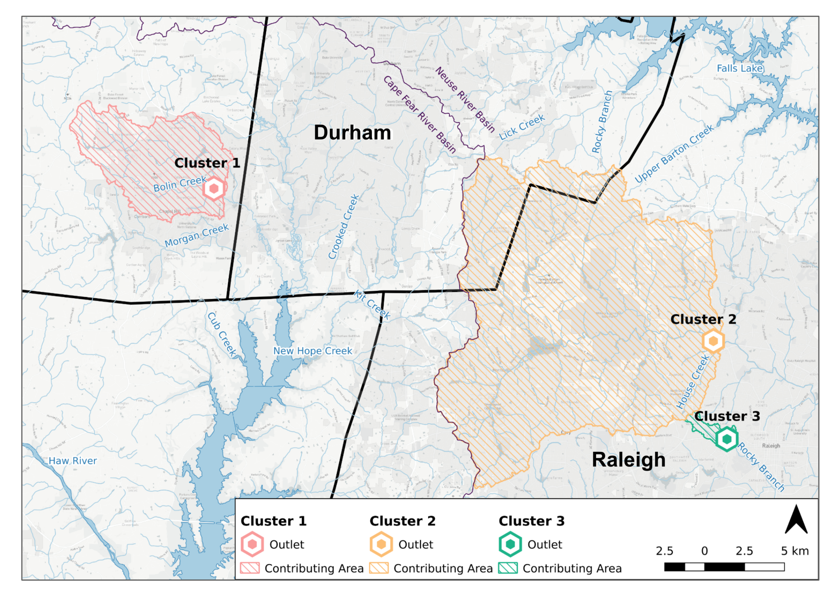
2.4.1. Analysis of Stormwater Problem Clusters
2.5. Spatially Filtered Fuzzy Cognitive Map
- Why might this location be a problem?
- What is the greatest barrier to resolving this problem?
- What actions can be taken to “fix” this problem?
“I think that the tributaries feeding into the [C]rabtree Creek need to be controlled by increasing riparian vegetation and decreasing the paved surface.”
What if we increase riparian buffers and decrease impervious surfaces?
3. Results
3.1. Individual Fuzzy Cognitive Maps of Stormwater Management
3.1.1. Analysis of Academic and Government FCM Indices
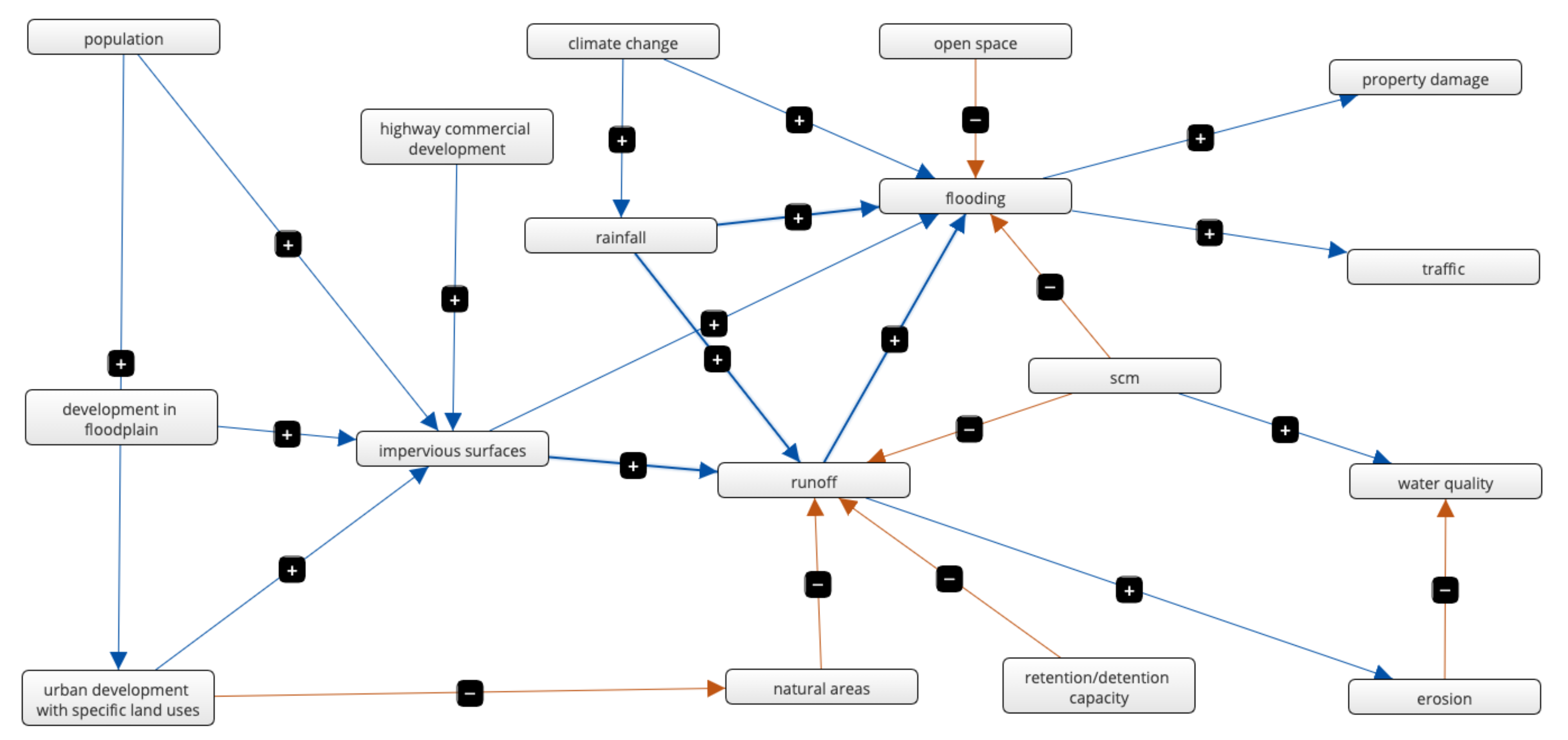
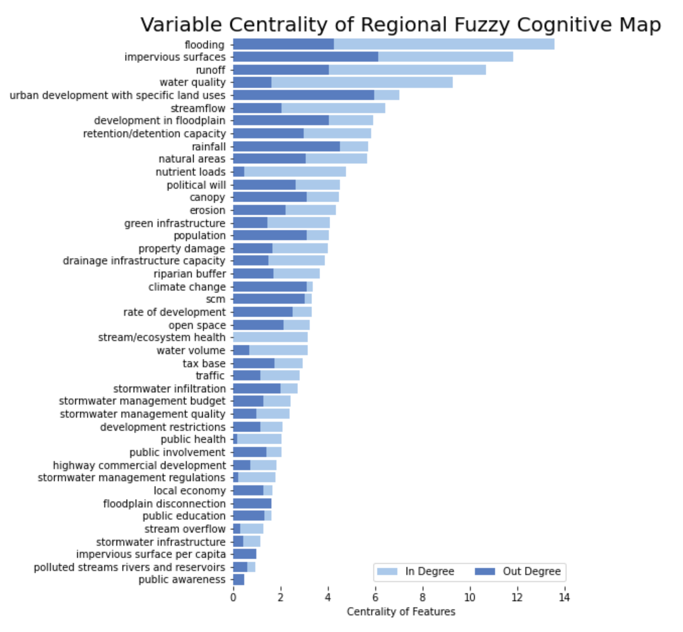
3.1.2. Regional Fuzzy Cognitive Map
3.2. Understanding Spatially Explicit Stormwater Problems
3.3. Problem Hotspots: Spatial Characteristics and Solutions
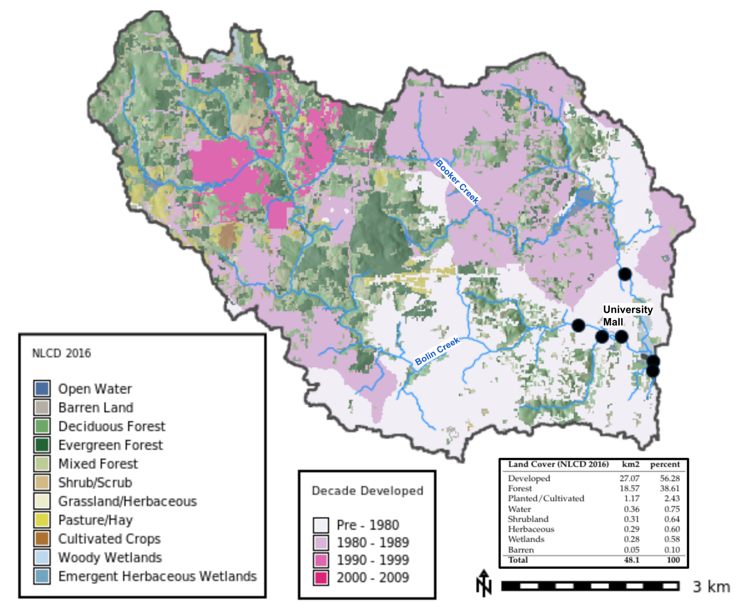
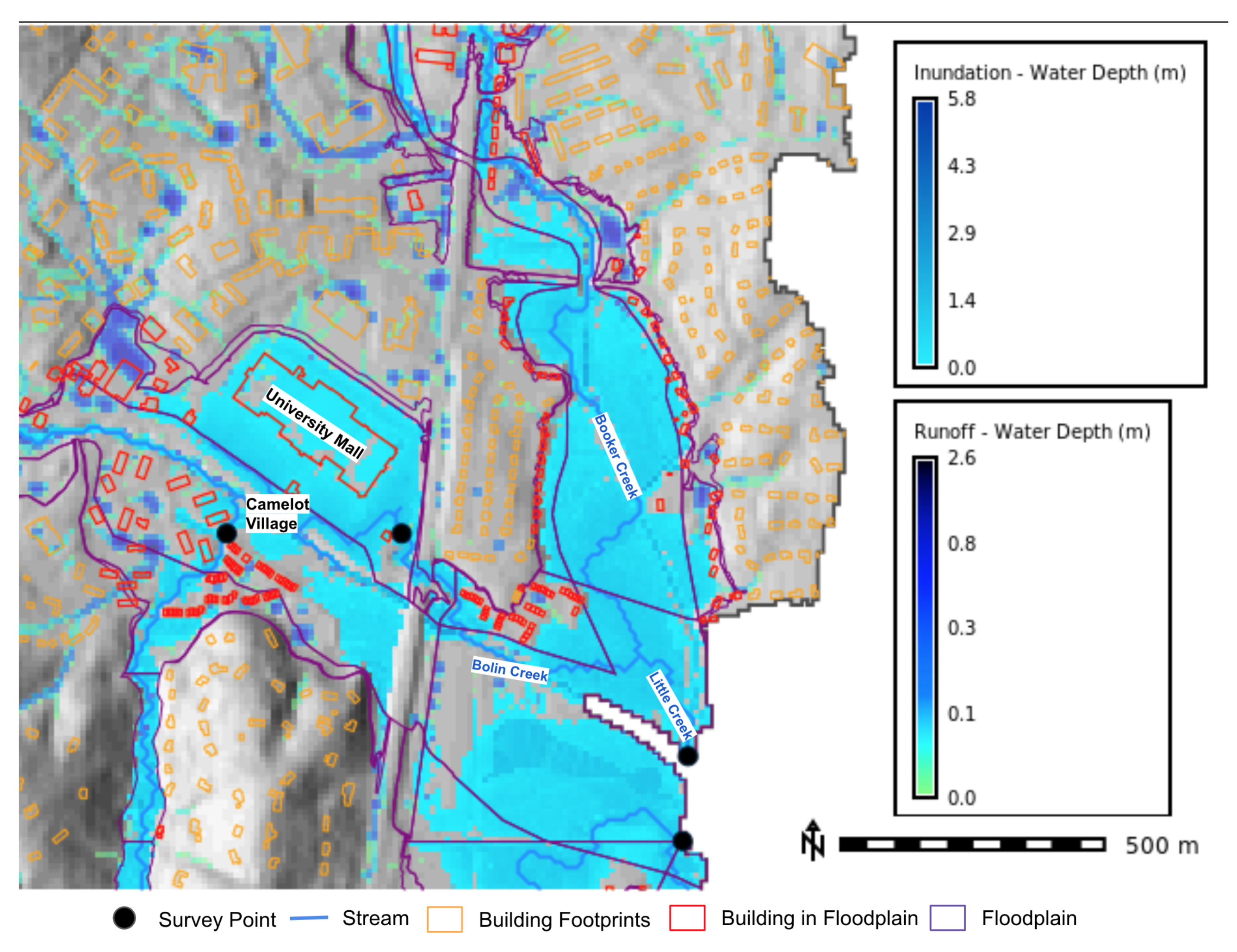
3.3.1. Cluster 1—University Mall
Problem
Barrier
Solution
- Increase retention/detention capacity
- Increase public education
- Increase stormwater control measures (SCM)
- Increase stormwater management budget
- Increase development restrictions
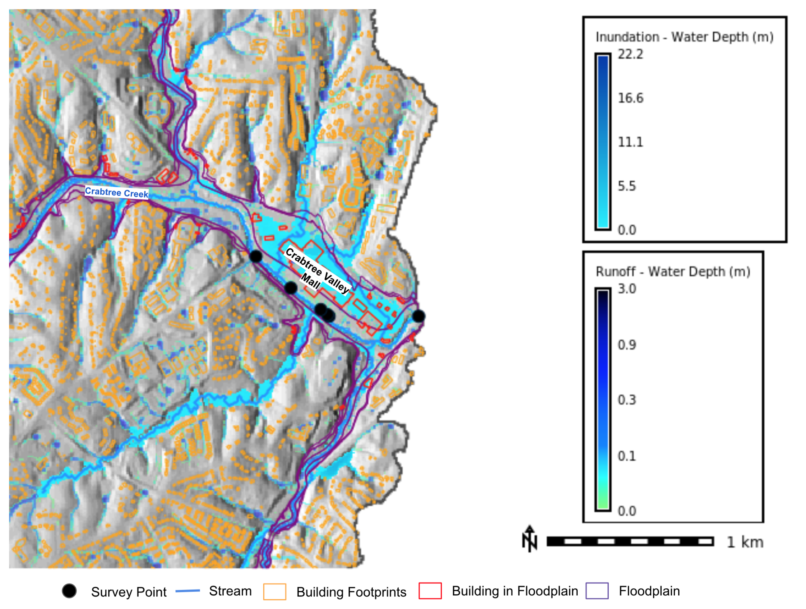
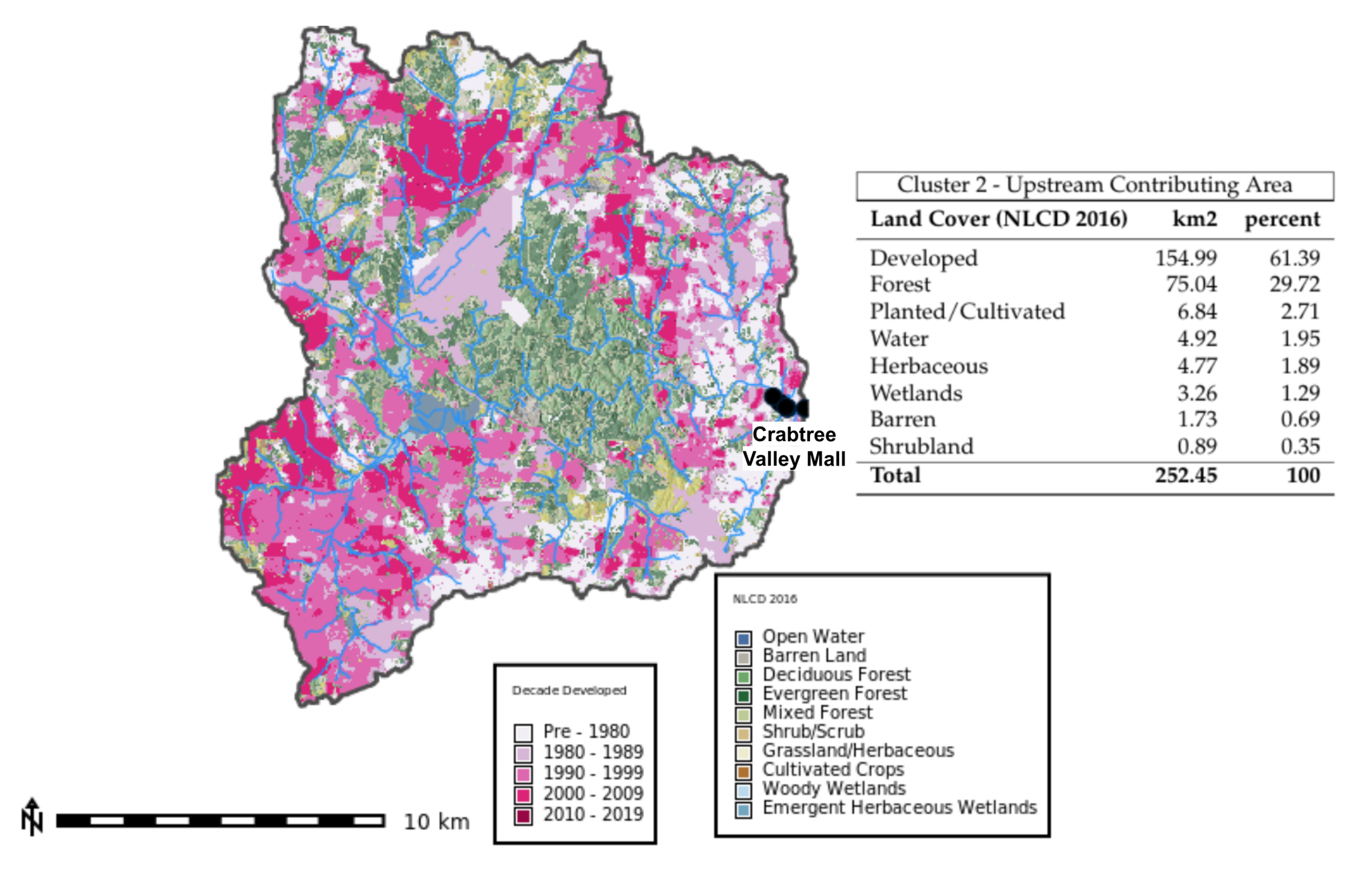
3.3.2. Cluster 2—Crabtree Valley Mall
Problem
Barrier
Solution
- Increase development restrictions
- Decrease impervious surfaces
- Increase floodplain mitigation
- Increase riparian buffer
- Increase stormwater infrastructure
- Increase transportation infrastructure
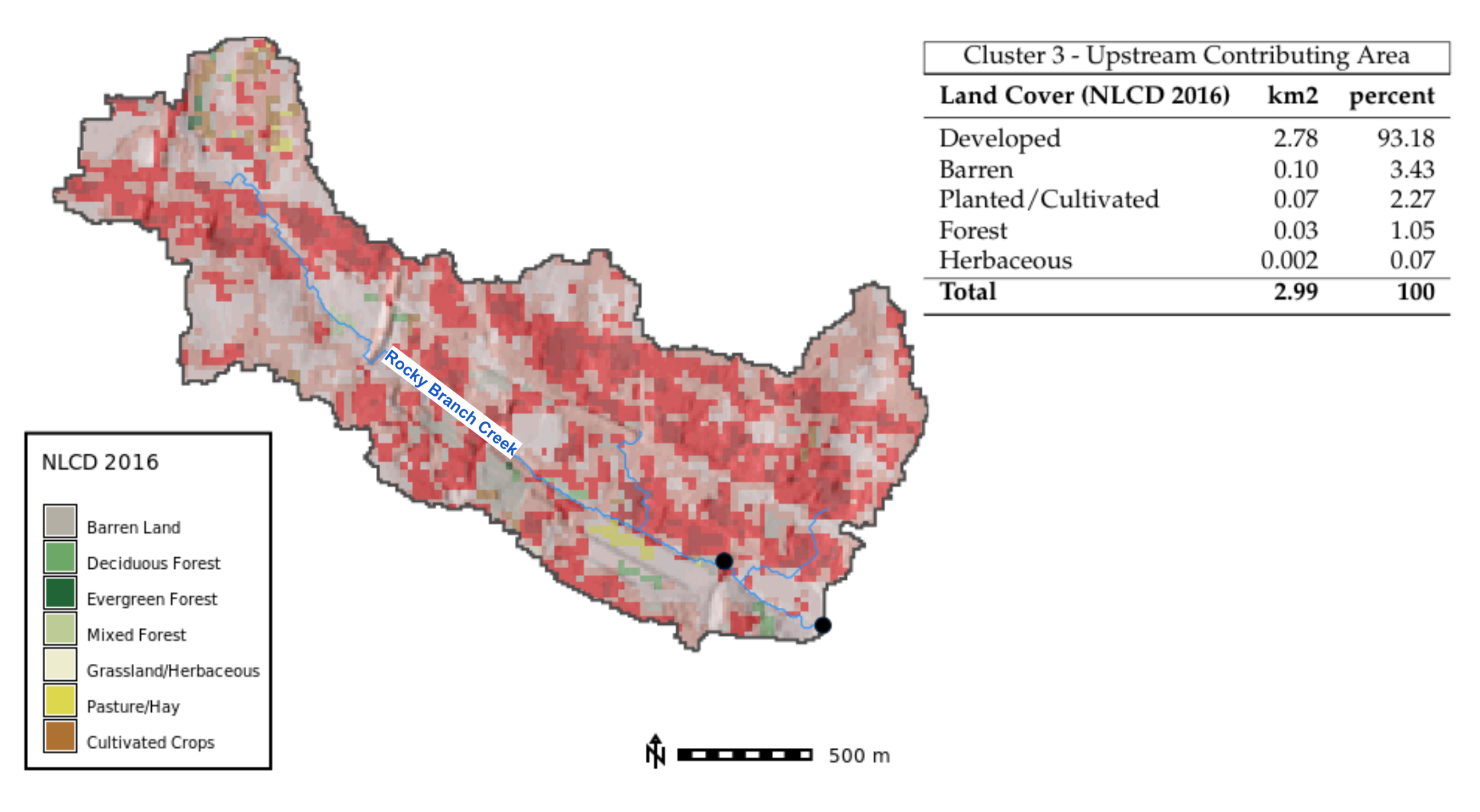
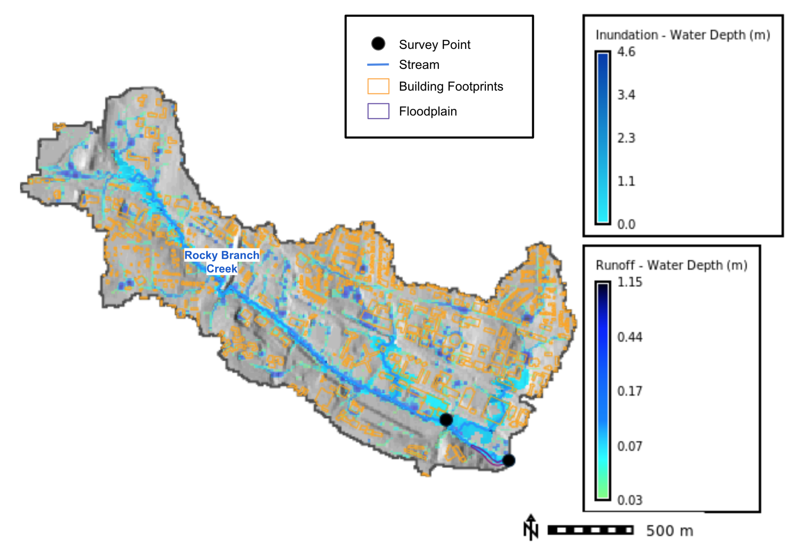
3.3.3. Cluster 3—North Carolina State University
Problem
“50 acres of land draining to a single 30 pipe”
Barrier
“How to fit a suitable sized pipe over a 10 foot tall underground tunnel”
Solution
4. Discussion
4.1. A Shared Understanding of Stormwater Management
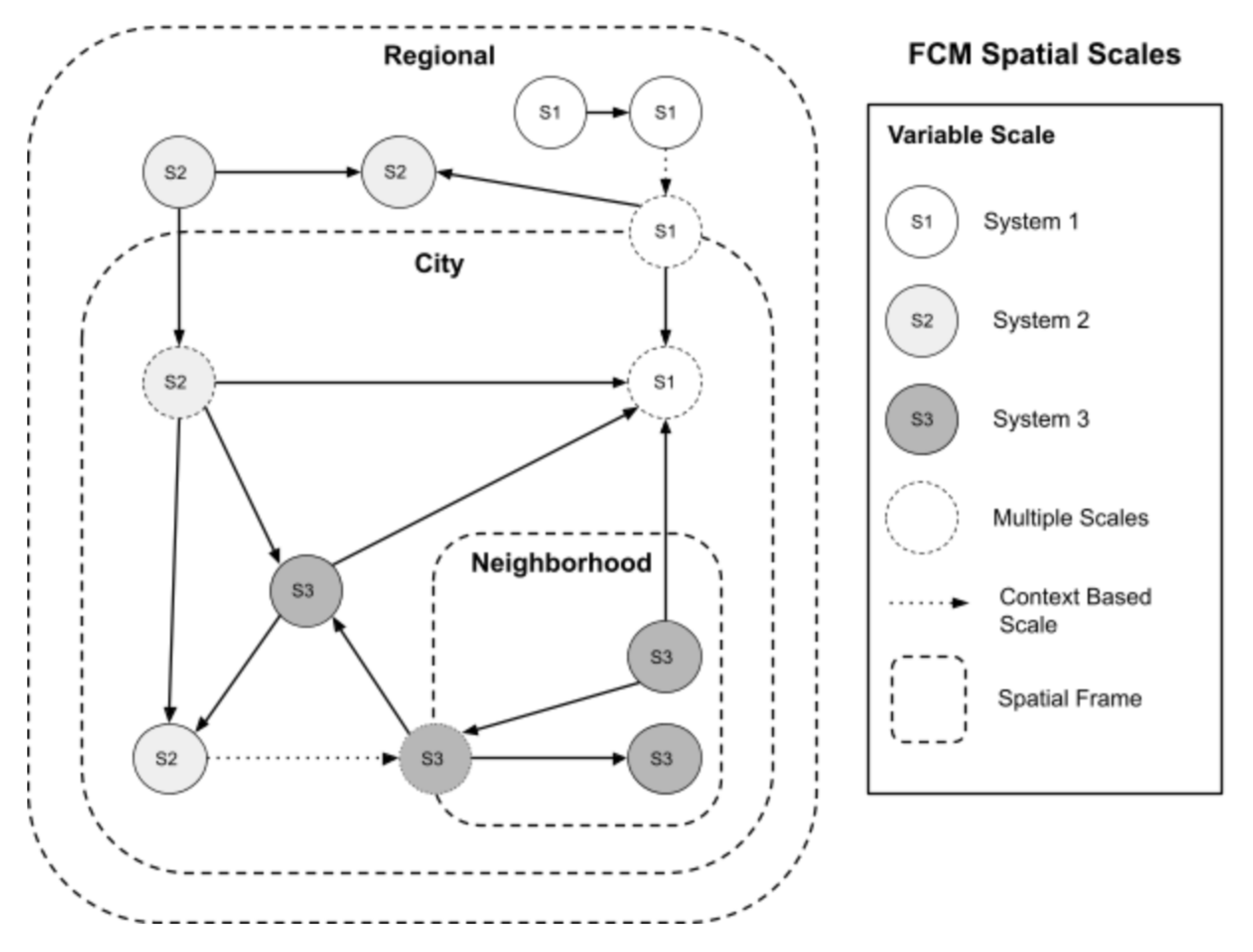
4.2. The Role of Spatial Scale on Fuzzy Cognitive Maps
4.3. Limitations
5. Conclusions
Author Contributions
Funding
Institutional Review Board Statement
Informed Consent Statement
Data Availability Statement
Acknowledgments
Conflicts of Interest
Appendix A. Regional Fuzzy Cognitive Maps
Appendix A.1. FCM Variable Contingency by Stakeholder Group

| FCM Variable Contingency Table | |||
|---|---|---|---|
| Variable | Academic (n = 7) | Government (n = 10) | Total |
| rainfall | 6.0 | 5.0 | 11 |
| flooding | 5.0 | 7.0 | 12 |
| impervious surfaces | 4.0 | 8.0 | 12 |
| climate change | 4.0 | 2.0 | 6 |
| retention/detention capacity | 3.0 | 3.0 | 6 |
| water quality | 3.0 | 3.0 | 6 |
| political will | 3.0 | 2.0 | 5 |
| runoff | 2.0 | 5.0 | 7 |
| population | 2.0 | 2.0 | 4 |
| stormwater management quality | 2.0 | NA | 2 |
| stormwater management regulations | 2.0 | NA | 2 |
| urban development with specific land uses | NA | 7.0 | 7 |
| property damage | NA | 5.0 | 5 |
| open space | NA | 4.0 | 4 |
| canopy | NA | 3.0 | 3 |
| development restrictions | NA | 3.0 | 3 |
| erosion | NA | 3.0 | 3 |
| natural areas | NA | 3.0 | 3 |
| stream/ecosystem health | NA | 3.0 | 3 |
| traffic | NA | 3.0 | 3 |
| development in floodplain | NA | 2.0 | 2 |
| green infrastructure | NA | 2.0 | 2 |
| highway commercial development | NA | 2.0 | 2 |
| local economy | NA | 2.0 | 2 |
| scm | NA | 2.0 | 2 |
| streamflow | NA | 2.0 | 2 |
| tax base | NA | 2.0 | 2 |
| Total | 36.0 | 85.0 | 121 |
References
- Cox, J. An Update on the Proposed Jordan Lake Nutrient Management Rules; City of Durham Stormwater Services Division. 2018. Available online: https://durhamnc.gov/DocumentCenter/View/3610 (accessed on 23 February 2021).
- Rittel, H.W.J.; Webber, M.M. Dilemmas in a General Theory of Planning. Policy Sci. 1973, 4, 155–169. [Google Scholar] [CrossRef]
- Gray, S.; Gagnon, A.; Gray, S.; O’Dwyer, B.; O’Mahony, C.; Muir, D.; Devoy, R.; Falaleeva, M.; Gault, J. Are coastal managers detecting the problem? Assessing stakeholder perception of climate vulnerability using Fuzzy Cognitive Mapping. Ocean. Coast. Manag. 2014, 94, 74–89. [Google Scholar] [CrossRef]
- Groffman, P.M.; Stylinski, C.; Nisbet, M.C.; Duarte, C.M.; Jordan, R.; Burgin, A.; Previtali, M.A.; Coloso, J. Restarting the conversation: Challenges at the interface between ecology and society. Front. Ecol. Environ. 2010, 8, 284–291. [Google Scholar] [CrossRef] [Green Version]
- Kosko, B. Fuzzy cognitive maps. Int. J. Man Mach. Stud. 1986, 24, 65–75. [Google Scholar] [CrossRef]
- Özesmi, U.; Özesmi, S.L. Ecological models based on people’s knowledge: A multi-step fuzzy cognitive mapping approach. Ecol. Model. 2004, 176, 43–64. [Google Scholar] [CrossRef] [Green Version]
- Voinov, A.; Jenni, K.; Gray, S.; Kolagani, N.; Glynn, P.D.; Bommel, P.; Prell, C.; Zellner, M.; Paolisso, M.; Jordan, R.; et al. Tools and methods in participatory modeling: Selecting the right tool for the job. Environ. Model. Softw. 2018, 109, 232–255. [Google Scholar] [CrossRef] [Green Version]
- Mouratiadou, I.; Moran, D. Mapping public participation in the Water Framework Directive: A case study of the Pinios River Basin, Greece. Ecol. Econ. 2007, 62, 66–76. [Google Scholar] [CrossRef]
- Voinov, A.; Kolagani, N.; McCall, M.K.; Glynn, P.D.; Kragt, M.E.; Ostermann, F.O.; Pierce, S.A.; Ramu, P. Modelling with stakeholders—Next generation. Environ. Model. Softw. 2016, 77, 196–220. [Google Scholar] [CrossRef]
- Gray, S.; Gray, S.; De Kok, J.L.; Helfgott, A.; O’Dwyer, B.; Jordan, R.; Nyaki, A. Using fuzzy cognitive mapping as a participatory approach to analyze change, preferred states, and perceived resilience of social-ecological systems. Ecol. Soc. 2015, 20, 11. [Google Scholar] [CrossRef]
- BenDor, T.K.; Kaza, N. A theory of spatial system archetypes. Syst. Dyn. Rev. 2012, 28, 109–130. [Google Scholar] [CrossRef]
- Elsawah, S.; Filatova, T.; Jakeman, A.J.; Kettner, A.J.; Zellner, M.L.; Athanasiadis, I.N.; Hamilton, S.H.; Axtell, R.L.; Brown, D.G.; Gilligan, J.M.; et al. Eight grand challenges in socio-environmental systems modeling. Socio Environ. Syst. Model. 2020, 2, 16226. [Google Scholar] [CrossRef] [Green Version]
- Vukomanovic, J.; Smart, L. GIS Participatory Modeling. Geogr. Inf. Sci. Technol. Body Knowl. 2021, 2021. [Google Scholar] [CrossRef]
- U.S. Census Bureau. Population, Population Change, and Estimated Components of Population Change: April 1, 2010 to July 1, 2019 (CO-EST2019-Alldata). 2021. Available online: https://www.census.gov/data/tables/time-series/demo/popest/2010s-counties-total.html (accessed on 10 June 2021).
- NCDEQ Stormwater Design Manual. 2017. Available online: https://files.nc.gov/ncdeq/Energy%20Mineral%20and%20Land%20Resources/Stormwater/BMP%20Manual/B%20%20Stormwater%20Calculations.pdf (accessed on 17 May 2021).
- Meentemeyer, R.K.; Mitasova, H.; Bendor, T.; Foy, K.; White, C.T. TomorrowNow Workshop 1 Report May 2018; Technical Report; Center for Geospatial Analytics at North Carolina State University. 2018. Available online: https://cnr.ncsu.edu/geospatial/wp-content/uploads/sites/12/2019/02/TomorrowNow-Workshop-1-Report.pdf (accessed on 30 January 2019).
- Hoffheimer, J. Triangle J Council of Governments: Regional Data Sharing Group. 2020. Available online: https://www.tjcog.org/partnerships/regional-data-sharing-group (accessed on 27 August 2021).
- Gray, S.A.; Gray, S.; Cox, L.J.; Henly-Shepard, S. Mental Modeler: A Fuzzy-Logic Cognitive Mapping Modeling Tool for Adaptive Environmental Management. In Proceedings of the 2013 46th Hawaii International Conference on System Sciences, Wailea, HI, USA, 7–10 January 2013; pp. 965–973. [Google Scholar] [CrossRef]
- Harary, N.; Norman, R.; Cartwright, D. Structural Models: An Introduction to the Theory of Directed Graphs; Wiley: New York, NY, USA, 1965. [Google Scholar]
- Aminpour, P. PyFCM: Python for Fuzzy Cognitive Mapping; 2018. Available online: https://github.com/tomorrownow/PyFCM (accessed on 4 June 2021).
- Bougon, M.; Weick, K.; Binkhorst, D. Cognition in Organizations: An Analysis of the Utrecht Jazz Orchestra. Adm. Sci. Q. 1977, 22, 606. [Google Scholar] [CrossRef]
- MacDonald, N. Trees and Networks in Biological Models; J. Wiley: Chichester, UK; West Sussex, NY, USA, 1983. [Google Scholar]
- Sandell, K. Sustainability in Theory and Practice: A Conceptual Framework of Eco-Strategies and a Case Study of Low-Resource Agriculture in the Dry Zone of Sri Lanka; Linkoeping University: Linkoeping, Sweden, 1996. [Google Scholar]
- Anderson, M.J. A new method for non-parametric multivariate analysis of variance. Austral Ecol. 2001, 26, 32–46. [Google Scholar] [CrossRef]
- Pearson, K.X. On the criterion that a given system of deviations from the probable in the case of a correlated system of variables is such that it can be reasonably supposed to have arisen from random sampling. Lond. Edinb. Dublin Philos. Mag. J. Sci. 1900, 50, 157–175. [Google Scholar] [CrossRef] [Green Version]
- Jaccard, P. The Distribution of the Flora in the Alpine Zone.1. New Phytol. 1912, 11, 37–50. [Google Scholar] [CrossRef]
- Morgan, C.J. Use of proper statistical techniques for research studies with small samples. Am. J. Physiol. Lung Cell. Mol. Physiol. 2017, 313, L873–L877. [Google Scholar] [CrossRef]
- Solana-Gutiérrez, J.; Rincón, G.; Alonso, C.; García-de Jalón, D. Using fuzzy cognitive maps for predicting river management responses: A case study of the Esla River basin, Spain. Ecol. Model. 2017, 360, 260–269. [Google Scholar] [CrossRef]
- Banini, G.; Bearman, R. Application of fuzzy cognitive maps to factors affecting slurry rheology. Int. J. Miner. Process. 1998, 52, 233–244. [Google Scholar] [CrossRef]
- Kokkinos, K.; Lakioti, E.; Papageorgiou, E.; Moustakas, K.; Karayannis, V. Fuzzy Cognitive Map-Based Modeling of Social Acceptance to Overcome Uncertainties in Establishing Waste Biorefinery Facilities. Front. Energy Res. 2018, 6, 112. [Google Scholar] [CrossRef] [Green Version]
- Felix, G.; Nápoles, G.; Falcon, R.; Froelich, W.; Vanhoof, K.; Bello, R. A review on methods and software for fuzzy cognitive maps. Artif. Intell. Rev. 2017. [Google Scholar] [CrossRef]
- Vukomanovic, J.; Skrip, M.M.; Meentemeyer, R.K. Making It Spatial Makes It Personal: Engaging Stakeholders with Geospatial Participatory Modeling. Land 2019, 8, 38. [Google Scholar] [CrossRef] [Green Version]
- Brown, G.; Weber, D. Public Participation GIS: A new method for national park planning. Landsc. Urban Plan. 2011, 102, 1–15. [Google Scholar] [CrossRef]
- Zolkafli, A.; Liu, Y.; Brown, G. Bridging the knowledge divide between public and experts using PGIS for land use planning in Malaysia. Appl. Geogr. 2017, 83, 107–117. [Google Scholar] [CrossRef]
- Meentemeyer, R.K.; Dorning, M.A.; Vogler, J.B.; Schmidt, D.; Garbelotto, M. Citizen science helps predict risk of emerging infectious disease. Front. Ecol. Environ. 2015, 13, 189–194. [Google Scholar] [CrossRef]
- Brown, G.; Weber, D.; de Bie, K. Is PPGIS good enough? An empirical evaluation of the quality of PPGIS crowd-sourced spatial data for conservation planning. Land Use Policy 2015, 43, 228–238. [Google Scholar] [CrossRef]
- Zolkafli, A.; Brown, G.; Liu, Y. An Evaluation of the Capacity-building Effects of Participatory GIS (PGIS) for Public Participation in Land Use Planning. Plan. Pract. Res. 2017, 32, 385–401. [Google Scholar] [CrossRef]
- Pereira, G.M. A Typology of Spatial and Temporal Scale Relations. Geogr. Anal. 2002, 34, 21–33. [Google Scholar] [CrossRef]
- GRASS Development Team. Geographic Resources Analysis Support System (GRASS GIS) Software; Open Source Geospatial Foundation: Chicago, IL, USA, 2021. [Google Scholar]
- Ester, M.; Kriegel, H.P.; Sander, J.; Xiaowei, X. A Density-Based Algorithm for Discovering Clusters in Large Spatial Databases with Noise; Number: CONF-960830; AAAI Press: Menlo Park, CA, USA, 1996. [Google Scholar]
- Jasiewicz, J.; Mickiewicz, A.; GRASS Development Team. Addon r.stream.basins. 2021. Available online: https://grass.osgeo.org/grass78/manuals/addons/r.stream.basins.html (accessed on 19 May 2021).
- Dewitz, J. National Land Cover Dataset (NLCD) 2016 Products. 2019. Available online: https://www.mrlc.gov/data/nlcd-2016-land-cover-conus (accessed on 10 June 2021).
- Mitasova, H.; Mitas, L.; Harmon, R. Simultaneous Spline Approximation and Topographic Analysis for Lidar Elevation Data in Open-Source GIS. Geosci. Remote. Sens. Lett. IEEE 2005, 2, 375–379. [Google Scholar] [CrossRef] [Green Version]
- Luke, A.; Sanders, B.F.; Goodrich, K.A.; Feldman, D.L.; Boudreau, D.; Eguiarte, A.; Serrano, K.; Reyes, A.; Schubert, J.E.; AghaKouchak, A.; et al. Going beyond the flood insurance rate map: Insights from flood hazard map co-production. Nat. Hazards Earth Syst. Sci. 2018, 18, 1097–1120. [Google Scholar] [CrossRef] [Green Version]
- Mitasova, H.; Thaxton, C.; Hofierka, J.; McLaughlin, R.; Moore, A.; Mitas, L. Path sampling method for modeling overland water flow, sediment transport, and short term terrain evolution in Open Source GIS. In Developments in Water Science; Elsevier: Amsterdam, The Netherlands, 2004; Volume 55, pp. 1479–1490. [Google Scholar] [CrossRef]
- Hofierka, J.; Knutová, M. Simulating spatial aspects of a flash flood using the Monte Carlomethod and GRASS GIS: A case study of the Malá Svinka Basin(Slovakia). Open Geosci. 2015, 7, 118–125. [Google Scholar] [CrossRef]
- Janssen, C. Manning’s n Values for Various Land Covers To Use for Dam Breach Analyses by NRCS in Kansas; Technical Report; NRCS: Wichita, KS, USA, 2016. Available online: https://rashms.com/wp-content/uploads/2021/01/Mannings-n-values-NLCD-NRCS.pdf (accessed on 19 May 2021).
- Bonnin, G.M.; Martin, D.; Lin, B.; Parzybok, T.; Yekta, M.; Riley, D. NOAA Atlas 14, 3rd ed.; U.S. Department of Commerce, National Oceanic and Atmospheric Administration, National Weather Service: Silver Spring, ML, USA, 2006; Volume 2, Version 3.0: Delaware, District of Columbia, Illinois, Indiana, Kentucky, Maryland, New Jersey, North Carolina, Ohio, Pennsylvania, South Carolina, Tennessee, Virginia, West Virginia.
- Nobre, A.D.; Cuartas, L.A.; Hodnett, M.; Rennó, C.D.; Rodrigues, G.; Silveira, A.; Waterloo, M.; Saleska, S. Height Above the Nearest Drainage—A hydrologically relevant new terrain model. J. Hydrol. 2011, 404, 13–29. [Google Scholar] [CrossRef] [Green Version]
- Tan, C.O.; Özesmi, U. A Generic Shallow Lake Ecosystem Model Based on Collective Expert Knowledge. Hydrobiologia 2006, 563, 125–142. [Google Scholar] [CrossRef] [Green Version]
- BenDor, T.K.; Salvesen, D.; Kamrath, C.; Ganser, B. Floodplain Buyouts and Municipal Finance. Nat. Hazards Rev. 2020, 21, 04020020. [Google Scholar] [CrossRef] [Green Version]
- Rahbek, C. The role of spatial scale and the perception of large-scale species-richness patterns. Ecol. Lett. 2005, 8, 224–239. [Google Scholar] [CrossRef]
- Meentemeyer, V.; Box, E.O. Scale Effects in Landscape Studies. In Landscape Heterogeneity and Disturbance; Turner, M.G., Ed.; Ecological Studies; Springer: New York, NY, USA, 1987; pp. 15–34. [Google Scholar] [CrossRef]
- Wiens, J.A. Spatial Scaling in Ecology. Funct. Ecol. 1989, 3, 385–397. [Google Scholar] [CrossRef]
- Iwanaga, T.; Wang, H.H.; Hamilton, S.H.; Grimm, V.; Koralewski, T.E.; Salado, A.; Elsawah, S.; Razavi, S.; Yang, J.; Glynn, P.; et al. Socio-technical scales in socio-environmental modeling: Managing a system-of-systems modeling approach. Environ. Model. Softw. 2021, 135, 104885. [Google Scholar] [CrossRef]
- Huck, J.J.; Whyatt, J.D.; Coulton, P. Spraycan: A PPGIS for capturing imprecise notions of place. Appl. Geogr. 2014, 55, 229–237. [Google Scholar] [CrossRef]
- United States Environmental Protection Agency. National Menu of Best Management Practices (BMPs) for Stormwater. 2015. Available online: https://www.epa.gov/npdes/national-menu-best-management-practices-bmps-stormwater (accessed on 28 September 2020).
- Arnstein, S.R. A Ladder Of Citizen Participation. J. Am. Inst. Planners 1969, 35, 216–224. [Google Scholar] [CrossRef] [Green Version]
- Basco-Carrera, L.; Warren, A.; van Beek, E.; Jonoski, A.; Giardino, A. Collaborative modelling or participatory modelling? A framework for water resources management. Environ. Model. Softw. 2017, 91, 95–110. [Google Scholar] [CrossRef]
- Phillips, J.D. The Role of Spatial Scale in Geomorphic Systems. Geogr. Anal. 1988, 20, 308–317. [Google Scholar] [CrossRef]
- Courty, L.G.; Pedrozo-Acuña, A.; Bates, P.D. Itzï (version 17.1): An open-source, distributed GIS model for dynamic flood simulation. Geosci. Model Dev. 2017, 10, 1835–1847. [Google Scholar] [CrossRef] [Green Version]
- Meentemeyer, R.K.; Tang, W.; Dorning, M.A.; Vogler, J.B.; Cunniffe, N.J.; Shoemaker, D.A. FUTURES: Multilevel Simulations of Emerging Urban—Rural Landscape Structure Using a Stochastic Patch-Growing Algorithm. Ann. Assoc. Am. Geogr. 2013, 103, 785–807. [Google Scholar] [CrossRef] [Green Version]


| Fuzzy Cognitive Maps Indices | |||||
|---|---|---|---|---|---|
| All | Academic | Government | ANOVA (p-Value) | Mann-Whitney (p-Value) | |
| Maps | 21 | 7 | 10 | ||
| Variables (N) | 13.2 ± 3.5 | 12.7 ± 4.3 | 13.5 ± 3.6 | 0.6909 | - |
| Connections (C) | 20.1 ± 8.0 | 16.9 ± 5.5 | 22.6 ± 10.0 | 0.1924 | - |
| Ordinary | 7.5 ± 2.6 | 8.1 ± 2.5 | 6.8 ± 2.5 | 0.2947 | - |
| Transmitters (T) | 3.6 ± 2.6 | 2.6 ± 2.2 | 4.4 ± 3.2 | - | 0.0667 |
| Receivers (R) | 2.1 ± 1.7 | 2.0 ± 2.4 | 2.3 ± 1.7 | - | 0.3440 |
| Complexity (R/T) | 0.8 ± 1.1 | 1.1 ± 1.7 | 0.7 ± 0.9 | - | 0.3831 |
| Hierarchy | 0.8 ± 0.3 | 0.7 ± 0.3 | 0.8 ± 0.2 | - | 0.1845 |
| Density | 0.1 ± 0.1 | 0.1 ± 0.1 | 0.2 ± 0.1 | - | 0.5 |
| Social Cognitive Model | Regional FCM | |
|---|---|---|
| Maps | 21 | 21 |
| Variables (N) | 124 | 43 |
| Connections (C) | 347 | 172 |
| Ordinary | 79 | 39 |
| Transmitters (T) | 27 | 3 |
| Receivers (R) | 18 | 1 |
| Complexity (R/T) | 0.7 | 0.33 |
| Hierarchy | 0.2 | 0.08 |
| Density | 0.02 | 0.09 |
Publisher’s Note: MDPI stays neutral with regard to jurisdictional claims in published maps and institutional affiliations. |
© 2021 by the authors. Licensee MDPI, Basel, Switzerland. This article is an open access article distributed under the terms and conditions of the Creative Commons Attribution (CC BY) license (https://creativecommons.org/licenses/by/4.0/).
Share and Cite
White, C.T.; Mitasova, H.; BenDor, T.K.; Foy, K.; Pala, O.; Vukomanovic, J.; Meentemeyer, R.K. Spatially Explicit Fuzzy Cognitive Mapping for Participatory Modeling of Stormwater Management. Land 2021, 10, 1114. https://doi.org/10.3390/land10111114
White CT, Mitasova H, BenDor TK, Foy K, Pala O, Vukomanovic J, Meentemeyer RK. Spatially Explicit Fuzzy Cognitive Mapping for Participatory Modeling of Stormwater Management. Land. 2021; 10(11):1114. https://doi.org/10.3390/land10111114
Chicago/Turabian StyleWhite, Corey T., Helena Mitasova, Todd K. BenDor, Kevin Foy, Okan Pala, Jelena Vukomanovic, and Ross K. Meentemeyer. 2021. "Spatially Explicit Fuzzy Cognitive Mapping for Participatory Modeling of Stormwater Management" Land 10, no. 11: 1114. https://doi.org/10.3390/land10111114