Article

Characterising Bedrock Aquifer Systems in Korea Using Paired Water-Level Monitoring Data

1
Department of Earth System Sciences, Yonsei University, Seoul 03722, Korea
2
National Groundwater Information Center, Korea Water Resources Corporation, Daejeon 34350, Korea
3
Division of Natural Resources Conservation, Korea Environment Institute, Sejong 30147, Korea
*
Author to whom correspondence should be addressed.
Water 2017, 9(6), 420; https://doi.org/10.3390/w9060420
Submission received: 5 March 2017 / Revised: 1 June 2017 / Accepted: 7 June 2017 / Published: 10 June 2017

Abstract

:
This study focused on characterising aquifer systems based on water-level changes observed systematically at 159 paired groundwater monitoring wells throughout Korea. Using spectral analysis, principal component analysis (PCA), and cross-correlation analysis with linear regression, aquifer conditions were identified from the comparison of water-level changes in shallow alluvial and deep bedrock monitoring wells. The spectral analysis could identify the aquifer conditions (i.e., unconfined, semi-confined and confined) of 58.5% of bedrock wells and 42.8% of alluvial wells: 93 and 68 wells out of 159 wells, respectively. Even among the bedrock wells, 50 wells (53.7%) exhibited characteristics of the unconfined condition, implying significant vulnerability of the aquifer to contaminants from the land surface and shallow depths. It appears to be better approach for deep bedrock aquifers than shallow alluvial aquifers. However, significant portions of the water-level changes remained unclear for categorising aquifer conditions due to disturbances in data continuity. For different aquifer conditions, PCA could show typical pattern and factor scores of principal components. Principal component 1 due to wet-and-dry seasonal changes and water-level response time was dominant covering about 55% of total variances of each aquifer conditions, implying the usefulness of supplementary method of aquifer characterisation. Cross-correlation and time-lag analysis in the water-level responses to precipitations clearly show how the water levels in shallow and deep wells correspond in time scale. No significant differences in time-lags was found between shallow and deep wells. However, clear time-lags were found to be increasing from unconfined to confined conditions: from 1.47 to 2.75 days and from 1.78 to 2.75 days for both shallow alluvial and deep bedrock wells, respectively. In combination of various statistical methods, three types of water-level fluctuation patterns were identified from the water-level pairs: Type I of identical aquifer systems (77.8%), Type II of the different aquifer systems with different recharge flow paths (9.5%), and Type III of unmatched aquifer system pairs and correlations (12.7%). Type I and II could be used as verification of aquifer condition in the paired monitoring system. However, Type III shows the complexity of water-level fluctuation in different aquifer conditions. This study showed that confined or not-confined conditions are not directly related to the depth of wells in the aquifer. Therefore, the utilisation of groundwater as a water-supply source should be carefully designed, tested for its hydrogeologic conditions, and managed to ensure sustainable quantity and quality.

1. Introduction

A groundwater monitoring system (e.g., water-level fluctuation, temperature, and water quality) provides essential information about short- and long-term changes in groundwater. Many countries have constructed groundwater monitoring systems and use the data to manage water resources [1,2,3]. Usually, a monitoring system considers the number, distribution, installation locations, and depths of wells. Much research using data obtained from groundwater monitoring has been reported. Examples include groundwater drought evaluation [4,5,6,7], studies of the relationship between climate change and groundwater [8,9], groundwater quality variables [10,11], seawater intrusion [12], and earthquake observation through groundwater analysis [13,14,15,16,17]. When interpreting groundwater monitoring data, fundamental information regarding the hydrogeological characteristics, the groundwater flow system, its fluctuations, and the connectivity of aquifers must be obtained and understood.
In Korea, the monitoring wells of the National Groundwater Monitoring Network (NGMN) have been constructed to provide general background data pertaining to the depth of domestic groundwater sources and to establish a systematic water resource management plan in the case that abnormalities occur in the water supply [18] (Figure 1). Therefore, the monitoring wells have not been installed from the perspective of clarifying aquifer characteristics of confined and unconfined systems, but rather to provide data to inform the utilisation of groundwater based on shallow alluvial and deep bedrock aquifers. Hence, the monitoring wells are classified by installation depths of around 30 m and 70 m, respectively. Where alluvial deposits are not well developed, monitoring wells were installed only in bedrock aquifers.
Various studies have used NGMN data to predict water-level through modelling methods [19], calculate recharge rates [20,21], and conduct long-term analyses of trends in climate change and water-level fluctuation [22,23]. However, most of these studies have simply classified the monitoring wells as alluvial and bedrock wells to compare the respective trends; the hydrogeologic characteristics of the aquifer system were not considered. In these studies, differences in the temporal-spatial changes at each monitoring well were interpreted based on depth factor. Considering the trends of global warming, water-resource shortages, and increasing risk from environmental pollution, emphasis should be placed on the sustainable management of groundwater with appropriate protective measures from known pollution sources at the land surface. From late 2010 to April 2011, a disastrous outbreak of foot and mouth disease (FMD) occurred in Korea. About four million animals were culled and buried in more than 4000 burial pits to prevent spread of the disease [24]. The burial sites are distributed widely and present a risk to groundwater contamination caused by the release of leachate. This is one reason why accurate aquifer characteristics are needed before exploitation of groundwater resources.
Groundwater in geologic formations is classified as confined, semi-confined, or unconfined based on the presence and permeability of any overlying formations which control water movement in and out of the aquifer, which result in different patterns of water-level fluctuations [25]. The confined status of an aquifer cannot be determined from the depth of the aquifer but should rather be based on a geological assessment that considers connectivity between the aquifer itself and any overlying formations. Generally, a confined aquifer lacks connectivity with the surface and is managed under the assumption that it is safe from any influx of contaminants from the surface. Therefore, the type of aquifer in which the monitoring well is installed should be defined accurately.
However, when exploiting bedrock groundwater in depth, the aquifer is often assumed to be confined without checking the water-level responses to natural precipitation while interpreting hydraulic test results [26,27]. When installing monitoring wells, the type of aquifer can be analysed by using the well logging data or through the pumping test. However, even these methods can be limited depending on site conditions (e.g., fractured rock aquifers), thus additional efforts are required. As an indirect alternative, a harmonic analysis of water-level data can be utilized. Natural water-level monitoring data include the intrinsic periodicities caused by earth tides and atmospheric pressure fluctuations, which influence the water-level fluctuations in confined, unconfined, and low-porosity aquifers [28,29,30]. Because the degree of influence can differ depending on the characteristics of each aquifer, the periodic features of such signals could be used to identify the type of aquifer more specifically [31,32,33].
In this study, deep bedrock aquifers in the NGMN, Korea, were re-interpreted to identify aquifer systems based on water-level fluctuation characteristics using various statistical approaches. The results regarding the confining status of aquifers could provide critical information on how to manage groundwater sustainably with proper protective measures.

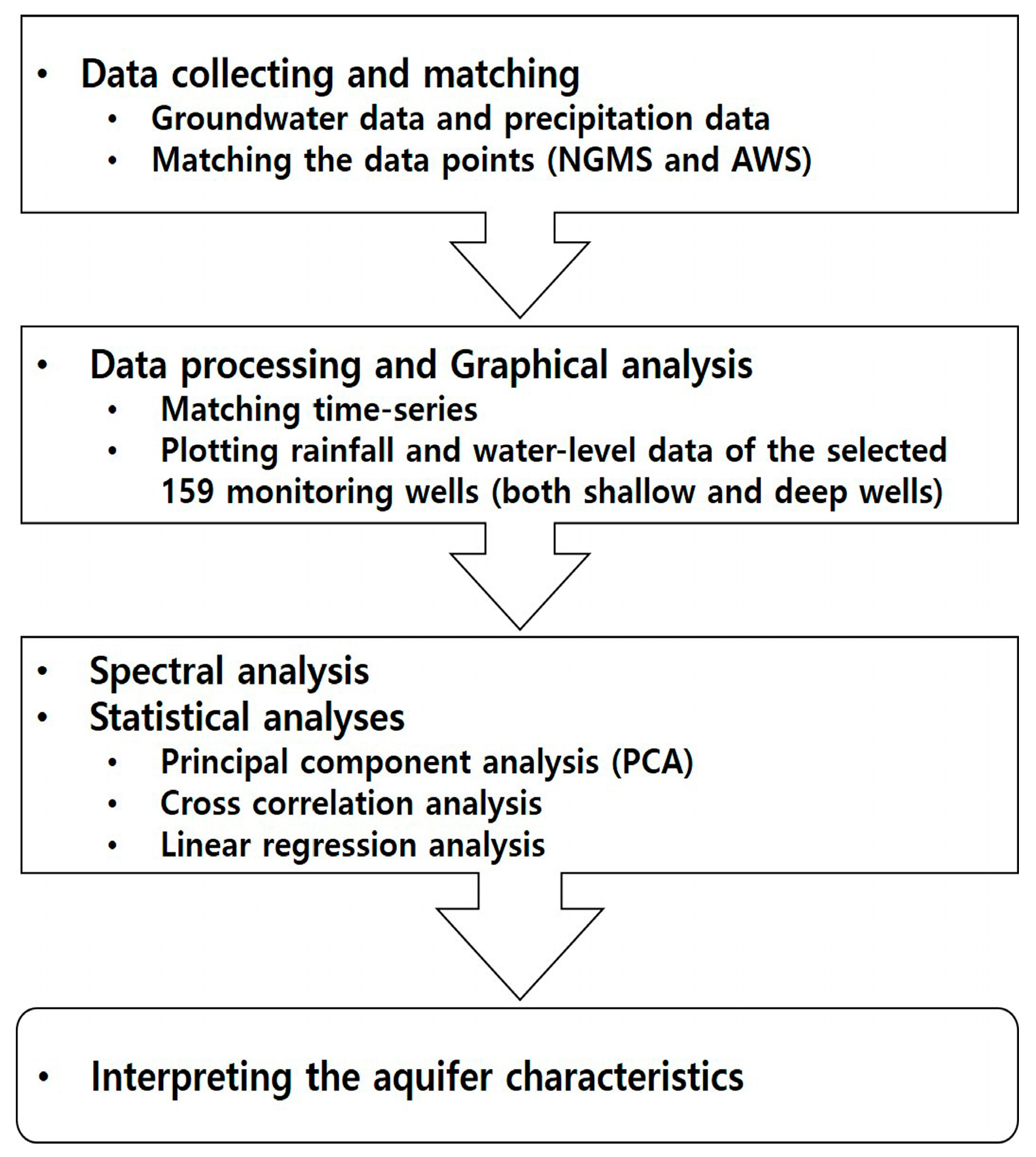
2. Data Acquisition and Methods

By 2010, bedrock monitoring wells had been implemented at 323 NGMN stations in the inland area. Among these, 159 stations also had alluvial monitoring wells [34] (Figure 1 and Table 1).
Each monitoring well is equipped with automatic data loggers to measure the water level, electrical conductivity, and temperature hourly (pressure sensors: Model Watermate (BAYTech Korea Inc., Seoul, Korea), with an accuracy of ±0.25% within the range 0–50 m and Model MK-15 CTD (HydroNet Co., Seongnam, Korea), with an accuracy of ±0.10% within the range 0–20 m; from [23]). For this study, the 159 stations with paired wells were selected for comparisons. An analysis was completed for each river basin.
Precipitation is the major source of groundwater recharge, causing water-level fluctuation with temporal and spatial variations. Thus, precipitation data were obtained from the 474 automatic weather stations (AWS) distributed locally at predetermined lattice points across the Korean Peninsula [35] (Figure 2).
The AWS stations located close to the monitoring wells were screened through computer matching, and the data from the matched stations were used for the correlation analysis with water-level fluctuations. The groundwater monitoring data from the NGMN and the precipitation data from the AWS were integrated and analysed in the following order (Figure 3):
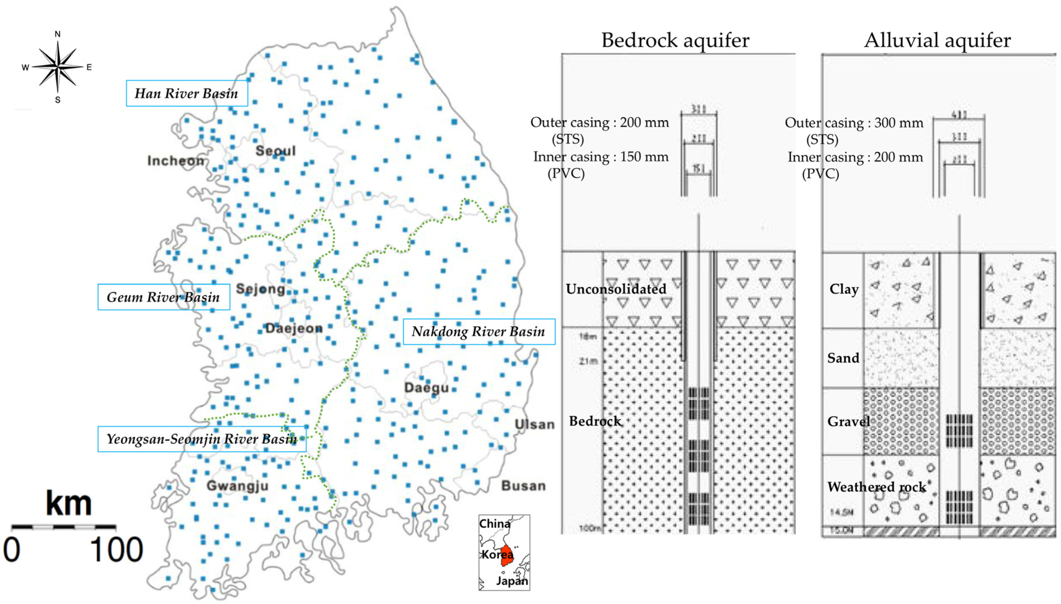
  • Considering spatial variations of precipitation and its impacts on groundwater levels, the AWS closest to the NGMN stations in the catchment were selected from the coordinates (Figure 2).
  • To analyse the temporal variations, both precipitation and groundwater monitoring data were processed to the same temporal unit of daily data.
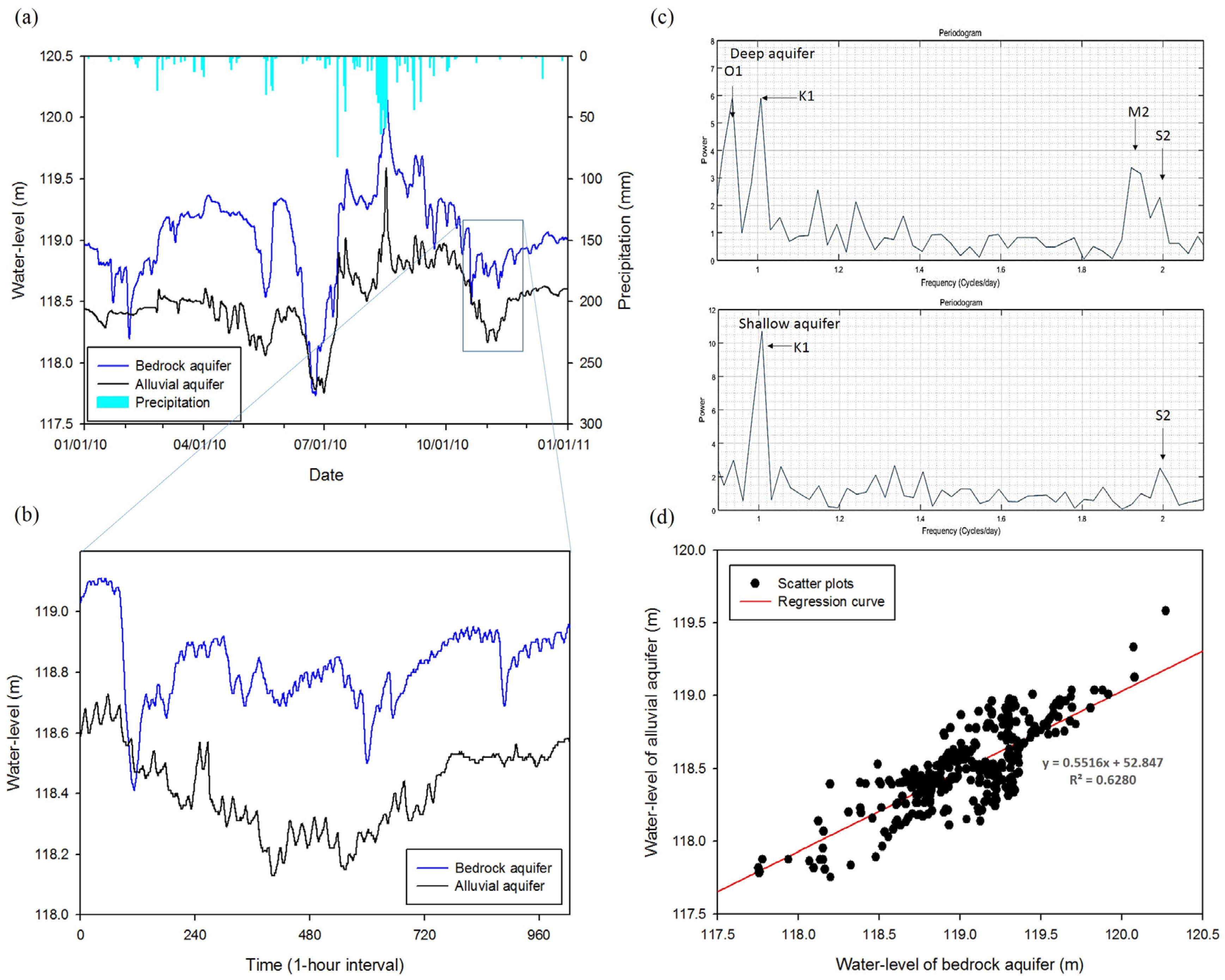
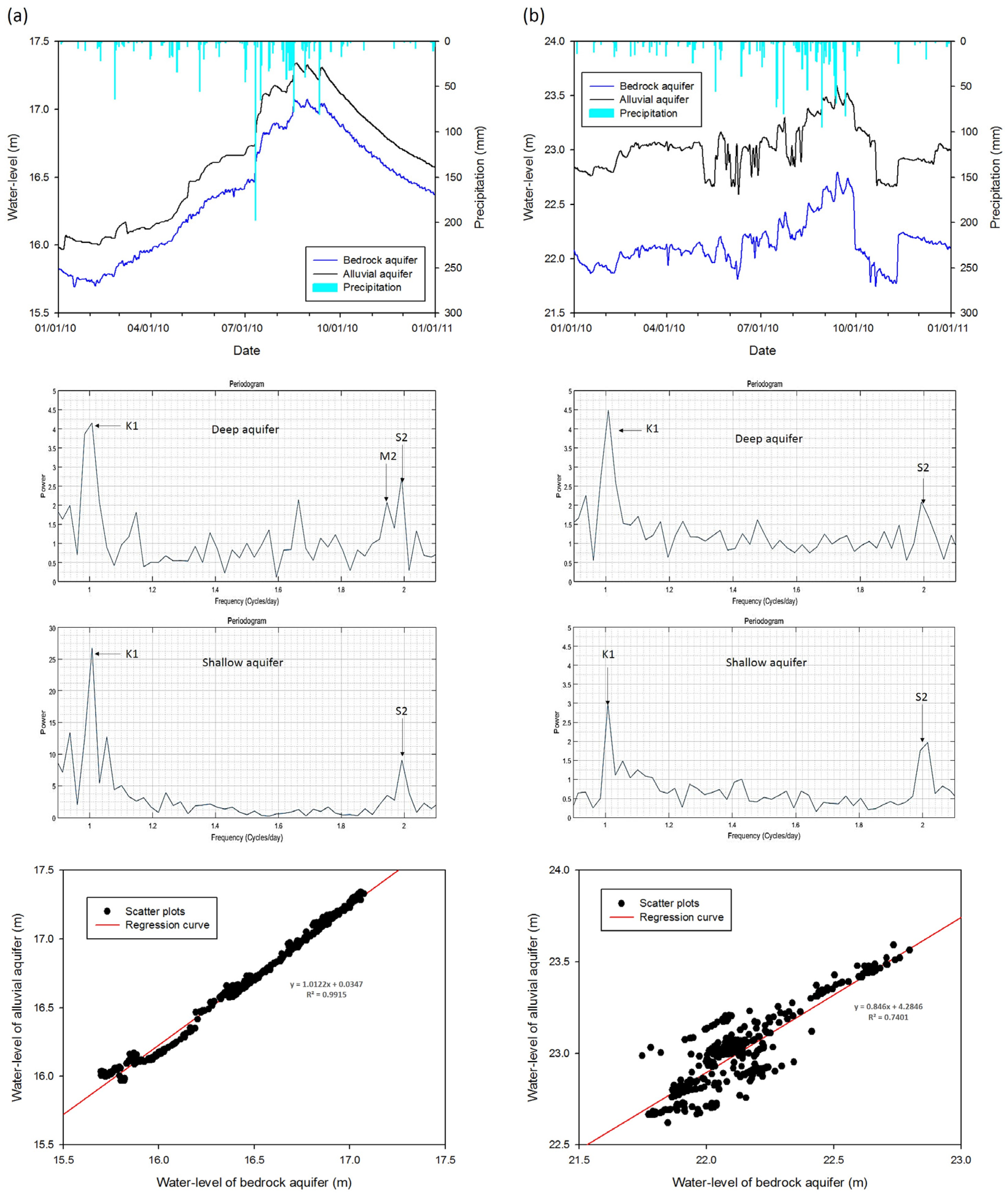
  • Using spectral analysis, the principal periodic components were extracted from the time-series data. This analysis used the hourly groundwater-level data during the dry season from February to April 2010 to minimise the noise caused by precipitation. Then, using the components, the characteristics of the aquifers were classified based on specific frequency domains, which are shown in the unconfined, semi-confined, and confined conditions [33]. In the study of water-level fluctuation, five major harmonic components of tidal potential are identified: S2, M2, N2, K1, and O1 [28,36] (Table 2).
    In an ideal unconfined condition, the response of the aquifer is the same as the effect from atmospheric pressure, and because the aquifer is not under pressure, earth tide signals or atmospheric signals do not exist [28,29]. However, if a vadose zone exists on top of the water table, lags can occur as the atmospheric changes pass through the vadose zone. The atmospheric signals of S2 and K1 occur by such lags [29], and the lack of an M2 signal can indicate an unconfined condition of an aquifer [33]. As the thickness of the vadose zone increases, the aquifer becomes contained by greater pressure and exhibits an M2 earth tide signature. In other words, even when an S2 signal is predominant and a K1 signal still exists, a weak M2 signal can lead to the interpretation of a semi-confined aquifer [32]. If the aquifer is confined under an impermeable layer, groundwater would be pressurized and a strong M2 signal, the earth tidal force, would be observed [28].
  • Using the daily average water-level data from the paired monitoring wells, the following statistical analyses were carried with the SPSS statistics program (Version 24, IBM® Corp., Armonk, NY, USA): (1) a principal component analysis (PCA) to characterize water-level fluctuation types of different aquifer conditions; (2) a cross-correlation analysis to analyse quantitatively the agreement of water-level fluctuations between the shallow and deep groundwater in paired wells with different aquifer conditions; (3) a lag-time analysis between precipitation and water-level responses of different aquifer types [37]; and (4) a linear regression analysis to confirm the fluctuation types of the two aquifers.
PCA is a multivariate statistical analysis for determining patterns and a technique that creates new variables called major components, the characteristic values and characteristic vectors of the matrix, through the spectral decomposition. By using the relationship between these variables, the features of the entire dataset can be explained [34,39].
Winter et al. [39] described how to apply PCA on groundwater hydrograph interpretation. PCA is used to reduce the dimensionality of interrelated variables using transforming the variables into a new set (i.e., principal components; PCs), which are uncorrelated [20]. “PCA quantifies the relationship between variables by computing the matrix of correlations for the entire dataset. The matrix of correlations is decomposed into a scores matrix and a loadings matrix by calculating and scaling eigenvectors and eigenvalues. PCs are linear combinations of the original variables that arise from the natural associations among the variables”, and defined as follow: (1) looking for the linear function; (2) calculating the eigenvectors and eigenvalues of the covariance matrix; (3) identifying systematic patterns of spatial and temporal variability in the original element (in this study, water-level) matrix; and (4) calculating the principal component loadings (PCL) and scores (PCS) that reflect the underlying covariance or correlation structure of the data.
PCL can be estimated as a measure of the spatial similarity between the water-level variables and each principal component, and PCS are an evaluation of the temporal similarity between the observed pattern of water levels for a given date and each principal component. Component scores are calculated as the inner product between a water-level data and a principal component. The component scores on an individual PC may have a zero as the mean value, a standard deviation equal to the component’s eigenvalue, and will be uncorrelated with the scores of all other components [39]. If the initial eigenvalues have high values, it means the proportion of the parent component group is relatively large. The “percent of variance” indicates the ratio of corresponding variables to the covariance, and the amount of variance interpreted by each eigenvalue [20].
Cross-correlation analysis is a method for obtaining the lag-time between two time-series. According to Box and Jenkins [40], the cross-correlation between two time-series x and y of length N is defined as Equation (1):
R x y ( k ) = i = 1 N k ( x i x ¯ ) ( y i + k y ¯ ) i = 1 N ( x i x ¯ ) 2 i = 1 N ( y i y ¯ ) 2
where Rxy(k) is the correlation coefficient at k, and the parameters x and y are the arithmetic means of length N, and N is the number of measurements. By calculating the value of k that maximises the correlation between the two time-series x and y, the lag-time can be determined.
In this study, PCA was used to characterize and validate the hydrographs of each aquifer type from the 63 pairs selected by the spectral analysis. Since water-level change and precipitation monitoring data were in hour and day units, respectively, in this study, lag-time between precipitation and water-level change was calculated in the unit of day.

3. Results

3.1. Analysis of Aquifer Type through Spectral Analysis

To apply the method of Rahi and Halihan [33] to the 159 paired monitoring wells, hourly measured time-series data were used to conduct a fast Fourier transform (FFT) analysis, producing a periodogram of the signal power of the frequency (cycles/day) [41,42,43]. Using the MATLAB® program (R2015a, Mathworks Inc., Natick, MA, USA), spectral analysis was conducted to classify the frequency domains and to analyse the strengths of the signals that were derived from the respective water-level data (Table S1). To minimise the influence of precipitation, which can act as noise, dry-season data from February to April 2010 were selected. Because the FFT method has a fundamental limitation in the number of time-series data for the analysis (being 2n), this study tried to use at least 2048 data points for processing. The spectral analysis could identify aquifer conditions of 93 and 68 monitoring wells (50.6% of the total 318 wells) for bedrock and alluvial aquifers, respectively (Table 3). For the rest, the signals were not clear enough to determine aquifer type, probably due to disturbances in the data continuity that caused by possible mechanical errors of monitoring equipment and the quarterly water-quality sampling processes.
Among the bedrock monitoring wells, 9 confined, 34 semi-confined, and 50 unconfined aquifer systems were identified (Table 3, Figure 4a). Among the alluvial monitoring wells, 4, 17 and 47 stations exhibited the characteristics of confined, semi-confined, and unconfined conditions, respectively (Figure 4b). The periodic components show clearer signals in the water-level data of the bedrock monitoring wells (58.5%) than those of the alluvial wells (42.8%). About 53.8% (50 out of 93 identified wells) of the deep bedrock monitoring wells exhibited the characteristics of an unconfined aquifer, and even four of shallow alluvial monitoring wells shown confined aquifer conditions. These findings clearly indicate that the characteristics of an aquifer system should not be assumed based on well depths. In this study, the number of significant components was determined by the criterion of cumulative percent, and about 80% of the variance was explained by three or four components for each aquifer condition. The hydrographs of the components were similar to the prior studies about the NGMN [20,44,45]. Among the computed components, the first principal component for the 63 pairs of monitoring wells was accounted for approximately 55% of the variance in the water-level data of each aquifer type (Table 4).
Figure 5 displays the time-series graph of the component scores for the first principal component (most dominant), and the examples of hydrograph for each aquifer condition as follows:
  • Component 1 for the unconfined aquifer: Seasonal changes between the dry season and the wet season are obvious. Water levels rise during precipitation events and decline after the wet season, following the form of an exponential function (Figure 5a).
  • Component 1 for the semi-confined aquifer: Seasonal changes appear between the dry season and the wet season, but the degree of water-level rise or decline is sharper than in PC1 of unconfined aquifer. The hydrograph pattern showed the intermediate form of the first component of unconfined and confined aquifer (Figure 5b).
  • Component 1 for the confined aquifer: The magnitude of the factor scores was two times greater than unconfined and semi-confined aquifer during the wet season, but the deviation of fluctuation pattern was less than one during the dry season. The hydrograph peak appeared after main precipitation events (Figure 5c).

3.2. Cross-Correlation Analysis

In this study, the daily average time-series of water-level data from the paired monitoring wells were correlated [37], and the resulting correlation coefficient was used to confirm the aquifer condition and the linkage between the two data pairs. When the time difference between the two datasets is shown as “0” the correlation coefficient becomes approximately 1, which implies that the two time-series data change simultaneously.
To identify the groundwater systems of bedrock aquifers, water-level fluctuations were compared with those from the alluvial wells for the 159 pairs. A total of 78.6% (125 stations) of pairs exhibited correlation coefficients above 0.9 (Table S1). The similarity of the water-level fluctuation pairs suggested that the groundwater in the deep bedrock and the shallow alluvial monitoring wells could be connected vertically, or at least not be fully separated [44]. Thus, the correlation coefficient could be used a supplementary to identify aquifer condition of paired wells with unclear periodic signals. For instance, in the case of a pair of wells with confined bedrock condition but unclear alluvial well in the spectral signal, if the correlation coefficient is greater than 0.9, the alluvial well must also be in confined condition.
Water-level changes in groundwater due to precipitation events are dependent on rainfall duration. The period of water-level rise could be even longer than the rainfall duration because of slow infiltration through pores of the geological matrix. Thus, the lag-time of water-level change due to precipitation event was calculated using the amount of daily precipitation and the daily-average water levels. The average lag times in the alluvial and bedrock monitoring wells were 1.77 days and 1.93 days, respectively (Table 5), indicating slightly faster responses in alluvial wells. Considering the average depths of those shallow alluvial and deep bedrock wells, about 30 m and 70 m, respectively, no significant difference occurs due to the depths of the monitoring wells.
In addition, among the 63 pairs that aquifer conditions were determined by the spectral analysis and PCA, the lag-times of each aquifer condition in bedrock wells (i.e., unconfined, semi-confined and confined) were estimated to be 1.78, 1.94 and 2.75 days, respectively (Table 5). The results showed that the lag-times were increasing from unconfined to confined conditions, clearly indicating that groundwater recharge takes more time from unconfined conditions to confined conditions.

4. Discussion

Spectral analysis based on the periodic components could identify unconfined, semi-confined and confined conditions of aquifer system in relatively deep bedrock monitoring wells than shallow alluvial wells. PCA of water-level fluctuation data from different aquifer conditions show significant differences in the first principal component, implying the usefulness of the method in characterising aquifer condition. Time-lag analyses further show the increasing water-level response time from unconfined to confined conditions of both unconfined and confined wells. Cross-correlation analysis could show how the water levels of shallow alluvial and deep bedrock wells in paired monitoring system correspond each other. Therefore, in combination of these various methods, three types of water-level fluctuation patterns could be drawn for the 63 pairs that aquifer conditions were clearly identified:
  • Type I (77.8%, 49 paired wells): Characterized by identical water-level fluctuation patterns in both shallow and deep groundwater, high correlation coefficients, and indistinguishable aquifer characteristics. Both alluvial and bedrock aquifers could be under the same unconfined or confined aquifer conditions (Figure 6).
  • Type II (9.5%, 6 paired wells): Characterized by low similarity between water-level fluctuations, low correlation coefficients, and clearly different aquifer characteristics. This implies that the shallow and deep aquifers are separated with different aquifer conditions. In this case, groundwater recharge could occur along different flow paths. That is, the water level in the deep bedrock wells could respond to horizontal recharge from up-gradient areas through fractures developed in the bedrock aquifer (Figure 7).
  • Type III (12.7%, 8 paired wells): As exceptions, three paired water-levels were similar in terms of high correlation coefficients with different periodic components, implying different aquifer characteristics. Even five paired data with low correlations, water-level fluctuations could become similar temporarily. This implies that groundwater flow pathways for recharge could vary depending on precipitation events (Figure 8).
Type I and II could be used as verification of aquifer condition in the paired monitoring system. However, Type III shows the complexity of water-level fluctuation in different aquifer conditions.
In Korea, the National Groundwater Information Center (GIMS) provides various information on the hydrogeological properties and the real-time information (e.g., water-level, temperature, electrical conductivity, etc.) for the groundwater monitoring wells of the NGMS, but does not provide information on the aquifer type (characteristics). Jeon et al. [46] analysed pumping-and-recovery test results for 314 observation wells of NGMS in Korea (112 alluvial and 202 bedrock aquifers) and reported that 83.7% wells (257/307; 7 wells had no data) show unconfined conditions, implying close connections between alluvial and bedrock aquifer systems. Results of this study with 71.4% of wells (85/119) in unconfined conditions conform relatively well to Jeon and co-workers’ results. However, they also noticed that some wells show different type of responses between pumping drawdowns and recovery plots, and those variations remain to be solved.

5. Conclusions

The hydrogeological characteristics of domestic aquifers need to be clarified to ensure the development and management of groundwater resources is sustainable. From a long-term perspective, these findings can inform systematic development and utilisation of groundwater resources, as well as the development of conservation management plans. This study focused on characterising the aquifer hydrogeological system based on water-level changes observed systematically from a total of 159 paired groundwater monitoring wells throughout Korea. Using statistical analyses, including spectral analysis, principal component analysis and cross-correlation analysis with linear regression, water-level changes in shallow alluvial and deep bedrock monitoring wells were analysed to identify their aquifer conditions.
Based on the periodic components, the spectral analysis could identify the aquifer conditions of 58.5% of wells in the bedrock aquifer and 42.8% of wells in alluvium: 93 and 68 wells out of 159 wells, respectively. This finding indicates that the spectral analysis on water-level responses is a relatively better approach for the bedrock aquifers than the alluvial aquifers [27,33,47]. However, still significant portions of the water-level changes remained unclear for categorising aquifer conditions, probably due to problems of data continuity occurred in the monitoring well maintenance and periodic sampling process.
Additionally, clearly identified confined conditions from the bedrock and alluvial monitoring wells were nine and four wells, respectively, indicating that confined or not-confined conditions are not directly related to the depth of wells in the aquifer. Even among the bedrock wells, 50 wells (53.7% of 93 wells with clear signals) exhibited characteristics of the unconfined condition, implying significant vulnerability of the aquifer to contaminants from the land surface and shallow depths. In contrast, only nine bedrock wells (9.7% of 93 wells with clear signals) exhibited fully confined aquifer characteristics.
PCA of water-level fluctuation shows the most significant principal component is PC1 that explains the about 55% of variance of all the unconfined, semi-confined, and confined aquifer conditions. PC1’s of each condition is significantly different from factor score and principal component pattern in aquifer conditions, implying the usefulness of the method in characterising aquifer condition.
Cross-correlation analysis could show how the water levels of shallow alluvial and deep bedrock wells in paired monitoring system correspond each other. Furthermore, time-lag analyses could show the increasing water-level response time from unconfined to semi-confined to confined conditions in both unconfined and confined wells, indicating interconnection of flow paths in various aquifer systems.
Consequently, combing various statistical methods, three types of water-level fluctuation patterns were identified for the 63 pairs of shallow alluvial and deep bedrock wells: Type I of identical aquifer systems (77.8%), Type II of the different aquifer systems with different recharge flow paths (9.5%), and Type III of unmatched aquifer system pairs and correlations (12.7%). Type I and II could be used as verification of aquifer condition in the paired monitoring system. However, Type III shows the complexity of water-level fluctuation in different aquifer conditions.
To utilize groundwater as a water supply source, it is necessary to maintain sufficient water quantity and appropriate water quality. Domestically, the contamination of surface water due to the emission of various industrial contaminants and long-term climate change with significant drought events escalate concerns about the systematic management of groundwater resources. As water quality issues raise public concerns, the demand for groundwater development from deep bedrock aquifers is increasing.
As shown in this study, aquifer conditions of confined-or-not are not dependent on the depth of wells, but should be inferred from hydrogeological conditions. Even in deep wells with depths greater than about 70 m (although it may not deep enough), more than 50% of wells are under unconfined conditions, and consequently under the influence of land-surface activities. Therefore, groundwater exploration in an underground aquifer system should be carefully designed, tested, and managed, and avoid the assumption that deep groundwater will remain sufficiently clean and plentiful over time.

Supplementary Materials

The following are available online at www.mdpi.com/2073-4441/9/6/420/s1. Table S1: Results of statistical analyses at each monitoring station.

Acknowledgments

The authors deeply appreciate the critical and constructive comments and suggestions from anonymous reviewers. This work was supported by the Korea Meteorological Industry Promotion Agency funded by the Korea Meteorological Administration Research and Development Program under grant “KMIPA 2015-6090” in Korea. The groundwater (NGMS) and precipitation (AWS) data for this work were obtained from the National Groundwater Information Management and Service Center and the Korea Meteorological Administration, respectively.

Author Contributions

Jae Min Lee and Nam C. Woo conceived and designed the research and wrote the paper; Jae Min Lee and Keunje Yoo analysed the data; and Chan-Jin Lee contributed raw data from the groundwater monitoring system.

Conflicts of Interest

The authors declare no conflict of interest.

References

  1. Taylor, C.J.; Alley, W.M. Ground-Water-Level Monitoring and the Importance of Long-Term Water-Level Data; Geological Survey (USGS): Reston, VA, USA, 2001; pp. 1–68.
  2. Lee, J.-Y.; Kwon, K.D. Current status of groundwater monitoring networks in Korea. Water 2016, 8, 168. [Google Scholar] [CrossRef]
  3. Nussbaumer, D.; Sutton, I.; Parker, A. Groundwater data management by water service providers in Peri-Urban areas of Lusaka. Water 2016, 8, 135. [Google Scholar] [CrossRef]
  4. Busciolano, R.J. Statistical Analysis of Long-Term Hydrologic Records for Selection of Drought-Monitoring Sites on Long Island, New York; Scientific Investigations Report 2004-5152; U.S. Geological Survey: Troy, NY, USA, 2005.
  5. Panda, D.K.; Mishra, A.; Jena, S.K.; James, B.K.; Kumar, A. The influence of drought and anthropogenic effects on groundwater levels in Orissa, India. J. Hydrol. 2007, 343, 140–153. [Google Scholar] [CrossRef]
  6. Li, B.; Rodell, M. Evaluation of a model-based groundwater drought indicator in the conterminous U.S. J. Hydrol. 2015, 526, 78–88. [Google Scholar] [CrossRef]
  7. Faunt, C.C.; Sneed, M.; Traum, J.; Brandt, J.T. Water availability and land subsidence in the Central Valley, California, USA. Hydrogeol. J. 2015, 24, 675–684. [Google Scholar] [CrossRef]
  8. Chen, Z.; Grasby, S.E.; Osadetz, K.G. Relation between climate variability and groundwater levels in the upper carbonate aquifer, Southern Manitoba, Canada. J. Hydrol. 2004, 290, 43–62. [Google Scholar] [CrossRef]
  9. Carter, R.C.; Parker, A.H. Climate change, population trends and groundwater in Africa. Hydrol. Sci. J. 2009, 54, 676–689. [Google Scholar] [CrossRef]
  10. Kurunc, A.; Ersahin, S.; Sonmez, N.K.; Kaman, H.; Uz, I.; Uz, B.Y.; Aslan, G.E. Seasonal changes of spatial variation of some groundwater quality variables in a large irrigated coastal Mediterranean region of Turkey. Sci. Total Environ. 2016, 554, 53–63. [Google Scholar] [CrossRef] [PubMed]
  11. Mohamed, M.M.A.; Hassane, A.B. Hydrochemistry assessment of groundwater quality in Al-Ain city, UAE. Environ. Earth Sci. 2016, 75, 353. [Google Scholar] [CrossRef]
  12. Melloul, A.J.; Goldenberg, L.C. Monitoring of seawater intrusion in coastal aquifers: Basics and local concerns. J. Environ. Manag. 1997, 51, 73–86. [Google Scholar] [CrossRef]
  13. Che, Y.; Yu, J.; Zhang, D.; Sun, Z.; Jian, C.; Peng, G. Annual regime characteristics of water level in bedrock wells in Beijing plain. Seismol. Geol. 1994, 163, 255–263. [Google Scholar]
  14. King, C.Y.; Azuma, S.; Ohno, M.; Asai, Y.; He, P.; Kitagawa, Y.; Igarashi, G.; Wakita, H. In search of earthquake precursors in the water-level data of 16 closely clustered wells at Tono, Japan. Geophys. J. Int. 2000, 1432, 469–477. [Google Scholar] [CrossRef]
  15. Kitagawa, Y.; Koizumi, N.; Takahashi, M.; Matsumoto, N.; Sato, T. Changes in groundwater levels or pressures associated with the 2004 earthquake off the west coast of northern Sumatra M9.0. Earth Planets Space 2006, 58, 173–179. [Google Scholar] [CrossRef]
  16. Lee, H.A.; Woo, N.C. Influence of the M9.0 Tohoku Earthquake on groundwater in Korea. Geosci. J. 2012, 16, 1–6. [Google Scholar] [CrossRef]
  17. Shalev, E.; Kurzon, I.; Doan, M.-L.; Lyakhovsky, V. Sustained water-level changes caused by damage and compaction induced by teleseismic earthquakes. J. Geophys. Res. Sol. Earth 2016, 121, 4943–4954. [Google Scholar] [CrossRef]
  18. Kim, N.J.; Cho, M.J.; Woo, N.C. Developing a National Groundwater Monitoring Network in Korea. Hydrogeol. J. 1995, 3, 89–94. [Google Scholar] [CrossRef]
  19. Yoon, H.; Kim, Y.; Ha, K.; Kim, G.B. Application of groundwater-level prediction models using data-based learning algorithms to National Groundwater Monitoring Network data. J. Eng. Geol. 2013, 23, 137–147. (In Korean) [Google Scholar] [CrossRef]
  20. Moon, S.K.; Woo, N.C.; Lee, K.S. Statistical analysis of hydrographs and water-table fluctuation to estimate groundwater recharge. J. Hydrol. 2004, 292, 198–209. [Google Scholar] [CrossRef]
  21. Cho, J.W.; Park, E. A study on delineation of groundwater recharge rate using water-table fluctuation and unsaturate zone soil water content model. J. Soil Groundw. Environ. 2008, 13, 67–76. (In Korean) [Google Scholar]
  22. Park, Y.C.; Jo, Y.J.; Lee, J.Y. Trends of groundwater data from the Korean National Groundwater Monitoring Stations: Indication of any change? Geosci. J. 2011, 15, 105–114. [Google Scholar] [CrossRef]
  23. Lee, B.; Hamm, S.Y.; Jang, S.; Cheong, J.Y.; Kim, G.B. Relationship between groundwater and climate change in South Korea. Geosci. J. 2014, 18, 209–218. [Google Scholar] [CrossRef]
  24. Kim, H.-S.; Kim, K. Microbial and chemical contamination of groundwater around livestock mortality burial sites in Korea—A review. Geosci. J. 2012, 16, 479–489. [Google Scholar] [CrossRef]
  25. Fetter, C.W. Applied Hydrogeology, 4th ed.; Prentice Hall: Upper Saddle River, NJ, USA, 2001. [Google Scholar]
  26. Veatch, A.C. Fluctuations of the Water Level in Wells, with Special Reference to Long Island, New York; Water Supply Paper 155; U.S. Geological Survey: Troy, NY, USA, 1906.
  27. Pachco, F.A.L.; Fallico, C. Hydraulic head response of a confined aquifer influenced by river stage fluctuations and mechanical loading. J. Hydrol. 2015, 531, 716–727. [Google Scholar] [CrossRef]
  28. Bredehoeft, J.D. Response of well-aquifer systems to earth tides. J. Geophys. Res. 1967, 72, 3075–3087. [Google Scholar] [CrossRef]
  29. Weeks, E.P. Barometric fluctuations in wells tapping deep unconfined aquifers. Water Resour. Res. 1979, 15, 1167–1176. [Google Scholar] [CrossRef]
  30. Freeze, R.A.; Cherry, J.A. Groundwater; Prentice Hall: Upper Saddle River, NJ, USA, 1979. [Google Scholar]
  31. Lambert, W.D. Report on earth tides. In U.S. Coast and Geodetic Survey, Special Publication; U.S. Government Printing Office: Washington, DC, WA, USA, 1940. [Google Scholar]
  32. Rahi, K.A. Estimating the Hydraulic Parameters of the Arbuckle-Simpson Aquifer by Analysis of Naturally-Induced Stresses. Ph.D. Thesis, Oklahoma State University, Stillwater, OK, USA, 2010. [Google Scholar]
  33. Rahi, K.A.; Halihan, T. Identifying Aquifer Type in Fractured Rock Aquifers using Harmonic Analysis. Ground Water 2013, 51, 76–82. [Google Scholar] [CrossRef] [PubMed]
  34. Ministry of Land, Transport and Maritime Affairs (MLTM). Korea Water Resources Corporation (K-Water); Groundwater Annual Report; MLTM: Daejeon, Korea, 2011. (In Korean) [Google Scholar]
  35. Korea Meteorological Administration (KMA). Annual Report of Automatic Weather Station Data; KMA: Seoul, Korea, 2012. [Google Scholar]
  36. Melchior, P. Earth Tides in Research in Geophysics; Version 2; Odishaw, H., Ed.; Massachusetts Institute of Technology Press: Cambridge, MA, USA, 1964; pp. 183–193. [Google Scholar]
  37. Davis, J.C. Statistics and Data Analysis in Geology, 2nd ed.; Wiley: New York, NY, USA, 1986. [Google Scholar]
  38. George, L.M. Introduction to Physical Oceanography; American Institute of Physics: College Park, MD, USA, 1996. [Google Scholar]
  39. Winter, T.C.; Mallory, S.E.; Allen, T.R.; Rosenberry, D.O. The use of principal component analysis for interpreting groundwater hydrographs. Ground Water 2000, 38, 234–246. [Google Scholar] [CrossRef]
  40. Box, G.E.P.; Jenkins, G.M. Time Series Analysis: Forecasting and Control; Holden-Day: San Francisco, CA, USA, 1976. [Google Scholar]
  41. Huang, N.E.; Shen, Z.; Long, S.R.; Wu, M.C.; Shih, H.H.; Zheng, Q.; Yen, N.-C.; Tung, C.C.; Liu, H.H. The empirical mode decomposition and the Hilbert spectrum for nonlinear and non-stationary time series analysis. Proc. R. Soc. Lond. A 1998, 454, 903–995. [Google Scholar] [CrossRef]
  42. Lynn, P.A.; Fuerst, W. Introductory Digital Signal Processing with Computer Application, 2nd ed.; John Wiley & Sons: Hoboken, NJ, USA, 1998. [Google Scholar]
  43. Shumway, R.H.; Stoffer, D.S. Time Series Analysis and its Applications: With R Examples, 3rd ed.; Springer: New York, NY, USA, 2011. [Google Scholar]
  44. Kim, G.B.; Yum, B.W. Classification and characterization for water level time series of shallow wells at the National Groundwater Monitoring Stations. J. Soil Groundw. Environ. 2007, 12, 86–97. (In Korean) [Google Scholar]
  45. Yi, M.J.; Kim, G.B.; Sohn, Y.C.; Lee, J.Y.; Lee, K.K. Time series analysis of groundwater level data obtained from national groundwater monitoring stations. J. Geol. Soc. Korea 2004, 40, 305–329. (In Korean) [Google Scholar]
  46. Jeon, S.-K.; Koo, M.-H.; Kim, Y.; Kang, I.-O. Statistical analysis of aquifer characteristics using pumping test data of National Groundwater Monitoring Wells for Korea. J. Soil Groundw. Environ. 2005, 10, 32–44. (In Korean) [Google Scholar]
  47. Boutt, D.F. Assessing hydrogeologic controls on dynamic groundwater storage using long-term instrumental records of water table levels. Hydrol. Process. 2017, 31, 1479–1497. [Google Scholar] [CrossRef]
Figure 1. Locations and schematic diagrams of the National Groundwater Monitoring Stations (modified from [2], www.gims.go.kr).
Water 09 00420 g001
Figure 2. Locations of the 159 well pairs among the National Groundwater Monitoring Stations (NGMS) and adjacent automatic weather stations (AWS) in the Korean Peninsula.
Water 09 00420 g002
Figure 3. Flow chart of the data analysis process for this study.
Water 09 00420 g003
Figure 4. Locations of the groundwater monitoring wells and analysed aquifer types from the various signal components: (a) bedrock aquifer; and (b) alluvial aquifer.
Water 09 00420 g004
Figure 5. Factor scores for the first principal component and groundwater hydrograph of the example site pairs of each aquifer characteristic: (a) unconfined aquifer, GimpoGimpo; (b) semi-confined aquifer, JecheonGoam; and (c) confined aquifer, SeoulMagok.
Water 09 00420 g005
Figure 6. Results of the correlation analysis and harmonic analysis of the paired water-level data from shallow and deep monitoring wells in 2010 for Type I with identical pattern, high correlation coefficient, and the same unconfined/confined aquifer: (a) groundwater hydrograph; (b) one-hour interval data for spectral analysis; (c) signal components; and (d) correlated data.
Water 09 00420 g006
Figure 7. Results of the correlation analysis and harmonic analysis of the paired water-level data from shallow and deep monitoring wells in 2010 for Type II with low similarity between water-level fluctuation pairs, low correlation coefficients and different aquifer characteristics: (a) groundwater hydrograph; (b) one-hour interval data for spectral analysis; (c) signal components; and (d) correlated data.
Water 09 00420 g007
Figure 8. Results of the correlation analysis and harmonic analysis of the paired water-level data from shallow and deep monitoring wells in 2010 for Type III with unmatched aquifer system pairs and correlation coefficients: (a) the different aquifer characteristic but high correlation coefficient; and (b) the same aquifer characteristic but low correlation coefficient.
Water 09 00420 g008
Table 1. National Groundwater Monitoring Stations in major river basins in Korea in 2010.
River BasinNo. of Monitoring StationsNo. of Stations with Paired Alluvial and Bedrock Monitoring WellsTotal Number of Wells
Han River10247149
Geum River7637113
Nakdong River9349142
Yeongsan–Seomjin River522678
Total323159482
Table 2. Principal periods by tide effects, type of aquifer, and expected response to various tides (modified from [33,38]).
Symbol (Signal Components)PeriodConfinedSemi-ConfinedUnconfinedDescription
M212.42 hPresent (dominant)PresentNot presentMain lunar
S212.00 hPresentPresent (dominant)May be presentMain solar
N212.66 hPresentMay be presentNot presentElliptical lunar
K123.93 hPresentPresentMay be presentSoli-lunar
O125.82 hPresentMay be presentNot presentMain lunar
Table 3. Aquifer characterisation for alluvial and bedrock monitoring wells based on the results of the spectral analysis.
ClassificationSignalAquifer CharacteristicMonitoring Well
BedrockAlluvial
ClearM2, K1, S2, (O1)Confined9 (5.7%)4 (2.5%)
K1, S2, M2, (O1)Semi-confined34 (21.4%)17 (10.7%)
K1, S2Unconfined50 (31.4%)47 (29.6%)
Not clearND *ND *66 (41.5%)91 (57.2%)
Overall--159 (100%)159 (100%)
* ND: Not determined.
Table 4. Total variance of water-level data as explained by the PCA from the 63 pairs of monitoring wells which characterized aquifer conditions by the spectral analysis.
ComponentInitial Eigenvalues
Unconfined AquiferSemi-Confined AquiferConfined Aquifer
Total% of VarianceCumulative% of VarianceTotal% of VarianceCumulative% of VarianceTotal% of VarianceCumulative% of Variance
154.68955.80555.80527.91154.72754.7277.26655.89655.896
215.61215.93071.7358.05015.78370.5101.67512.88468.779
35.3075.41577.1505.56310.90881.4181.1929.17177.950
44.3214.40981.560------
Table 5. Results of the lag-time for depths and aquifer conditions.
Aquifer TypeLag-Time (in Units of Days)
Depth UnconfinedSemi-ConfinedConfinedAverage
Shallow alluvial well1.47 ± 0.20 (n = 30)2.18 ± 0.78 (n = 10)2.75 ± 1.11 (n = 4)1.77 ± 0.24
Deep bedrock well1.78 ± 0.31 (n = 23)1.94 ± 0.50 (n = 16)2.75 ± 1.11 (n = 4)1.93 ± 0.26

