
A New Method for Evaluating Riverside Well Locations Based on Allowable Withdrawal


Abstract
:1. Introduction
2. Methodology
2.1. Groundwater Flow Model
2.2. Arrangement of Well Locations
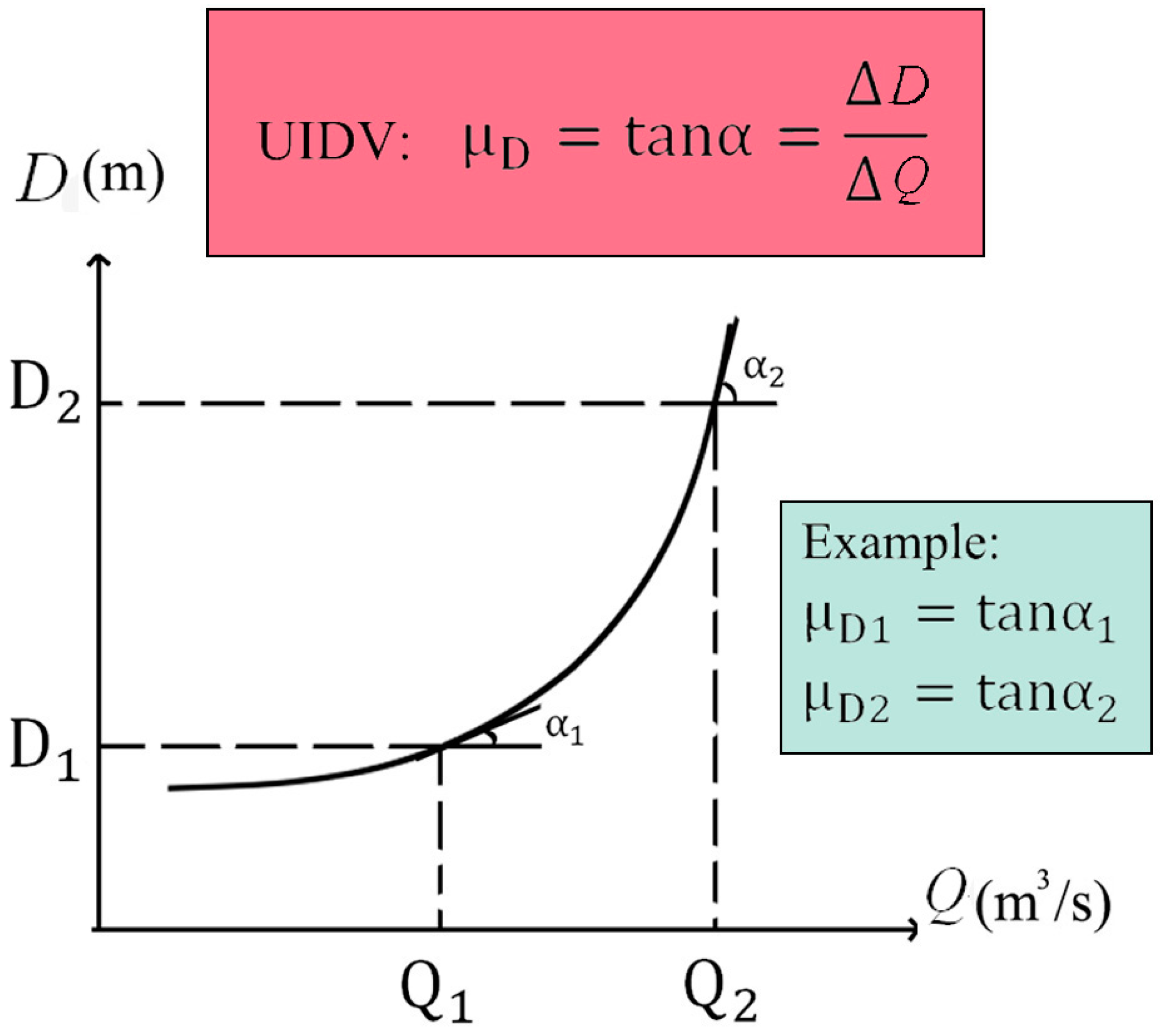
2.3. Unity Increased Drawdown Value (UIDV)
2.4. Method for Evaluating the Well Location Arrangement
- Low observed drawdown;
- A low value of UIDV;
- A stable UIDV.
- Maximum value of UIDV: this is used to evaluate whether the magnitude of change in drawdown is appropriate. Based on the maximum drawdown, the standard value of UIDV is set to be the minimum thickness of the aquifer (26.7 m/(m3/s)).
- Stability standard of UIDV: this parameter is used to evaluate whether the sequence of UIDV has recursive relationships. We determined that the sequence should be monotonic, or close to it. If the sequence of UIDV is monotonically increasing (or decreasing), it is possible to predict that the trend in drawdown would increase (or decrease) when a basic unit value was added in any extraction scenario.
3. Application and Discussion
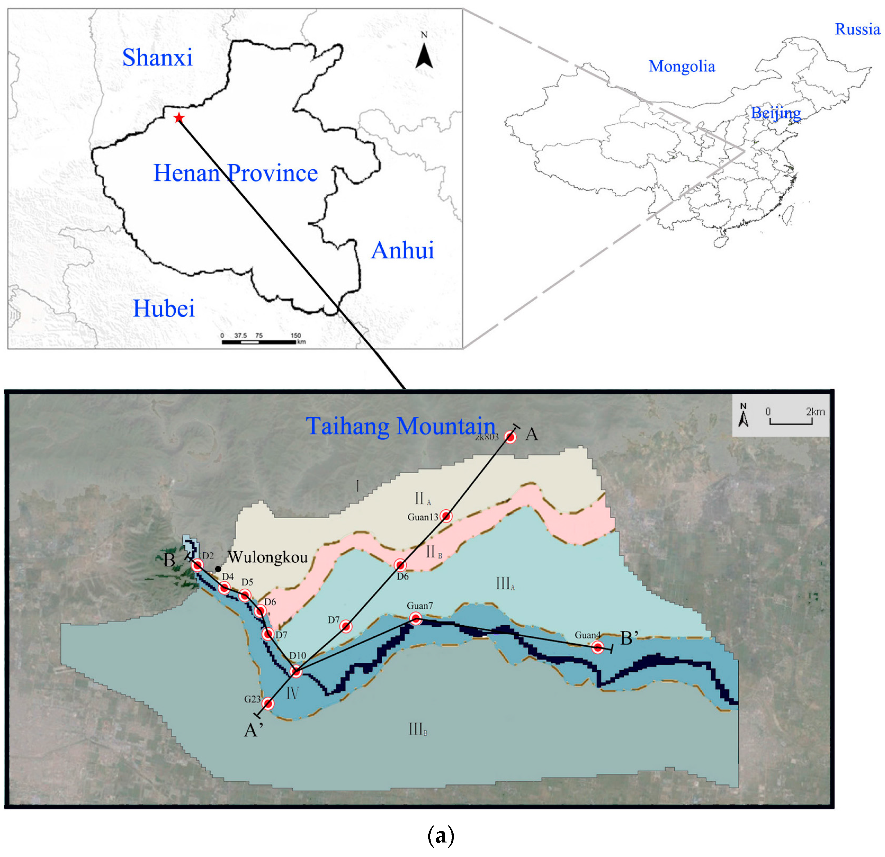
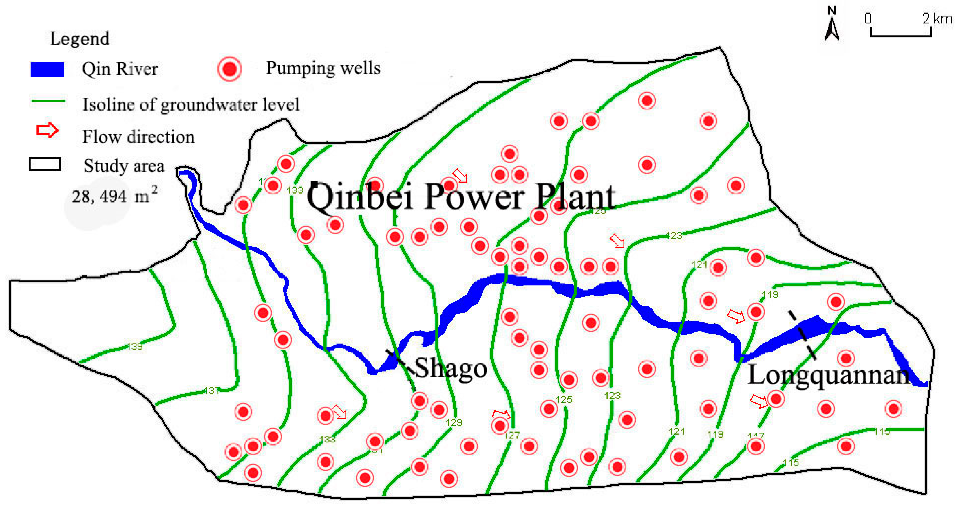
3.1. Study Area
- Mountainous area (part I): this area consists of the Taihang Mountains. This part contains terrain that is 250–750 m higher than that at the well field, and a distinct topography is present in the southern region.
- Alluvial area (part II): this area is located near the Taihang Mountains, and it can be divided into two sub-parts according to the topography, namely:
- Part IIA: a zonal distribution from west to east. The width from north to south is about 3–4 km. The length from west to east is about 8–9 km. The lithology consists of stone and pebble.
- Part IIB: a fringe along the alluvial area. The width from north to south is about 1–2 km. The length from west to east is about 8–9 km. The lithology consists of pebble and gravel.
- Low-lying area (part III): this area can be divided into two sub-parts according to the topography, namely:
- Part IIIA: an area located along the left bank of the Qin River. The width from north to south is about 3–5 km. The ground elevation ranges from 135 to 142 m (from west to east). The lithology consists of round gravel.
- Part IIIB: an area located along the right bank of the Qin River. The width from north to south is about 5–7 km. The length from west to east is about 20 km. The lithology consists of loam.
- Valley area (part IV): this area is located in the valley of the Qin River. The width of the floodplain ranges from 200 to 500 m. Gravel is distributed around the valley, and sand covers the ground in the downstream reaches of the Qin River.
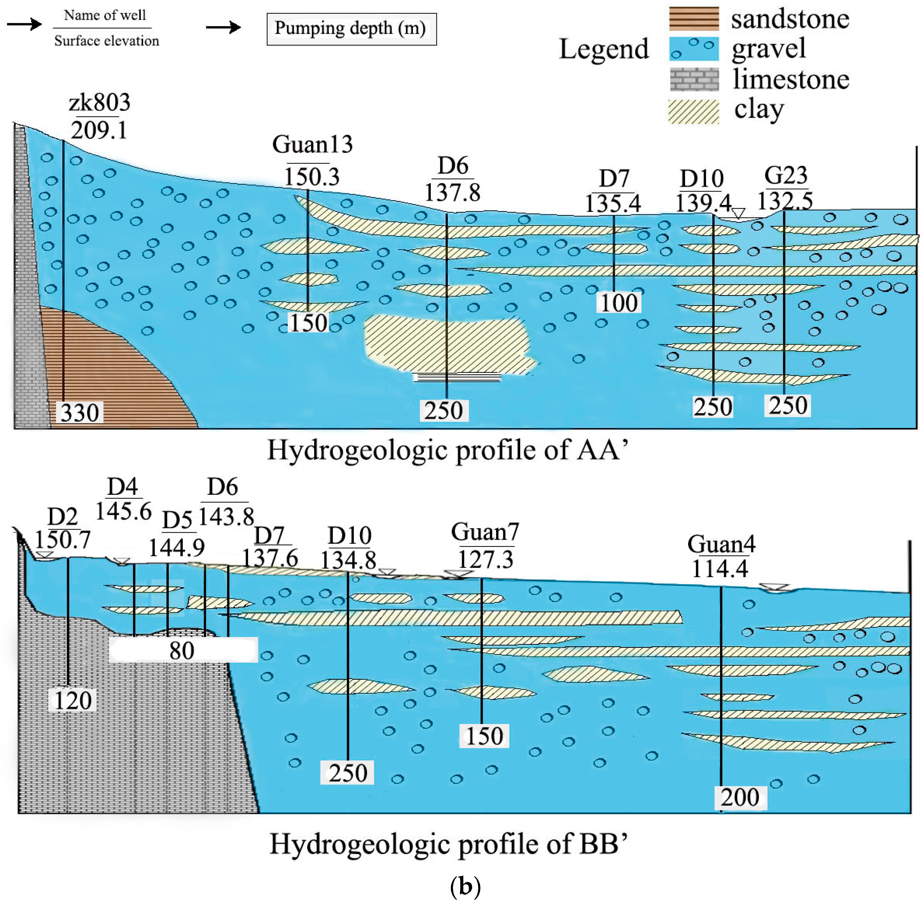
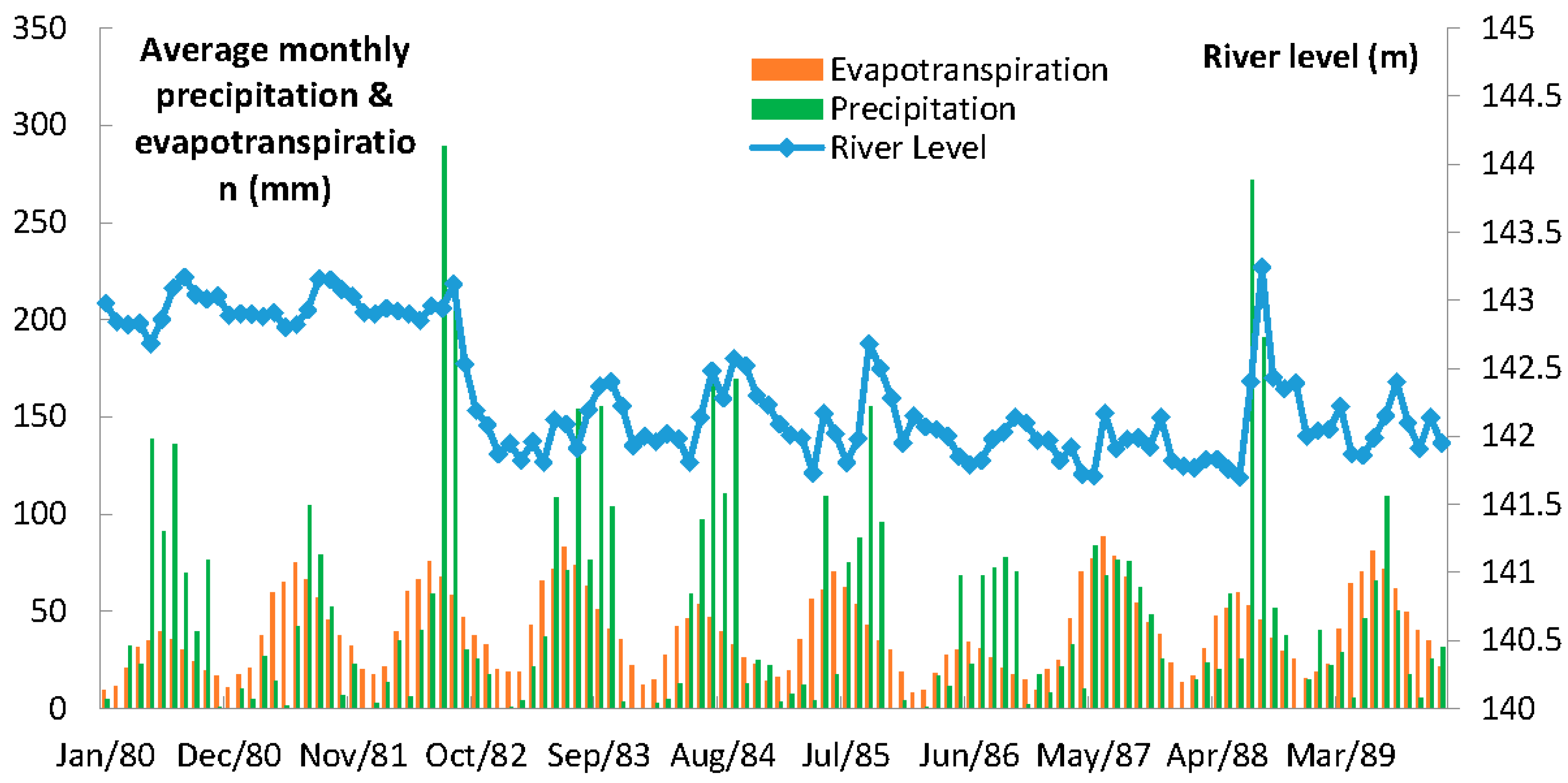
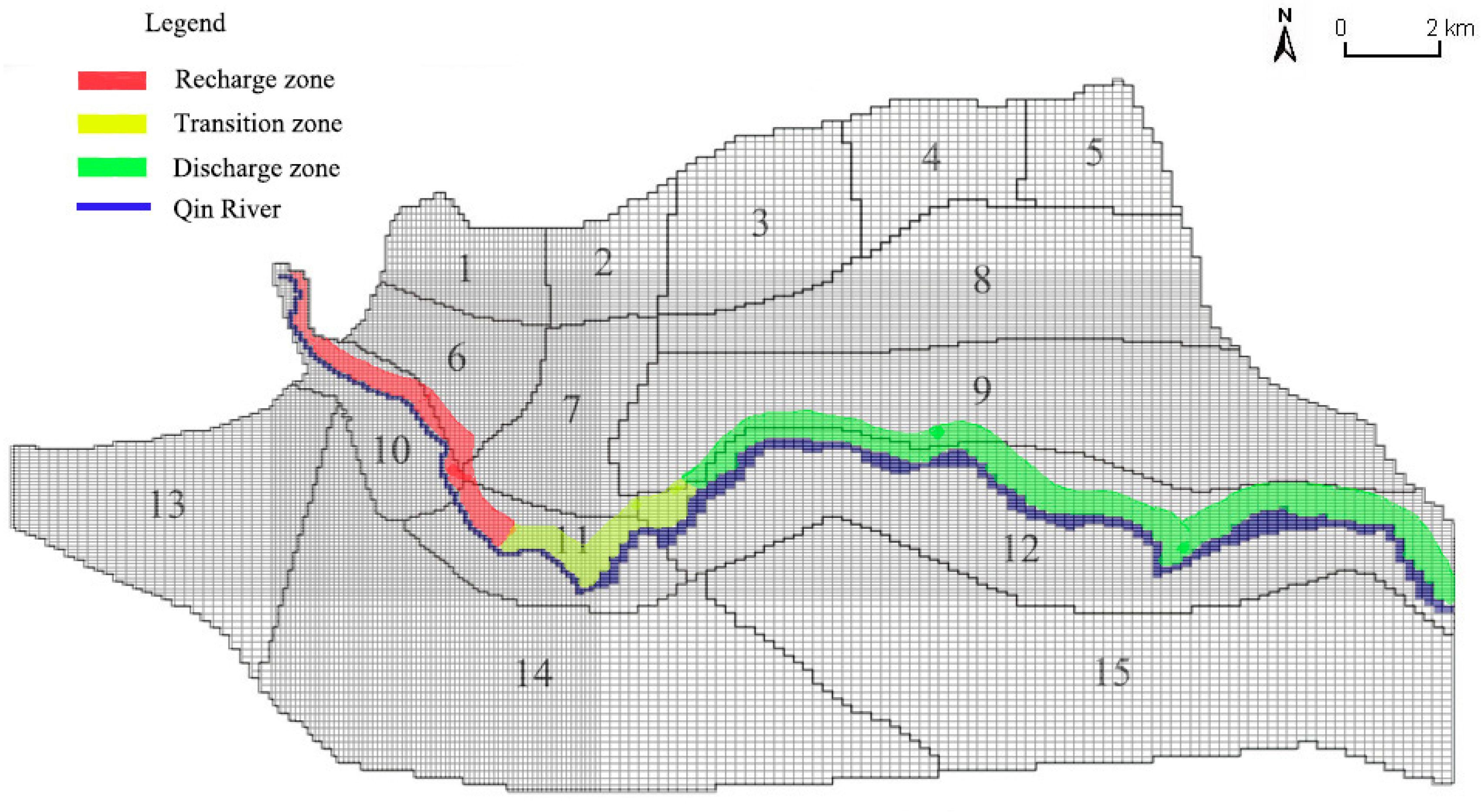
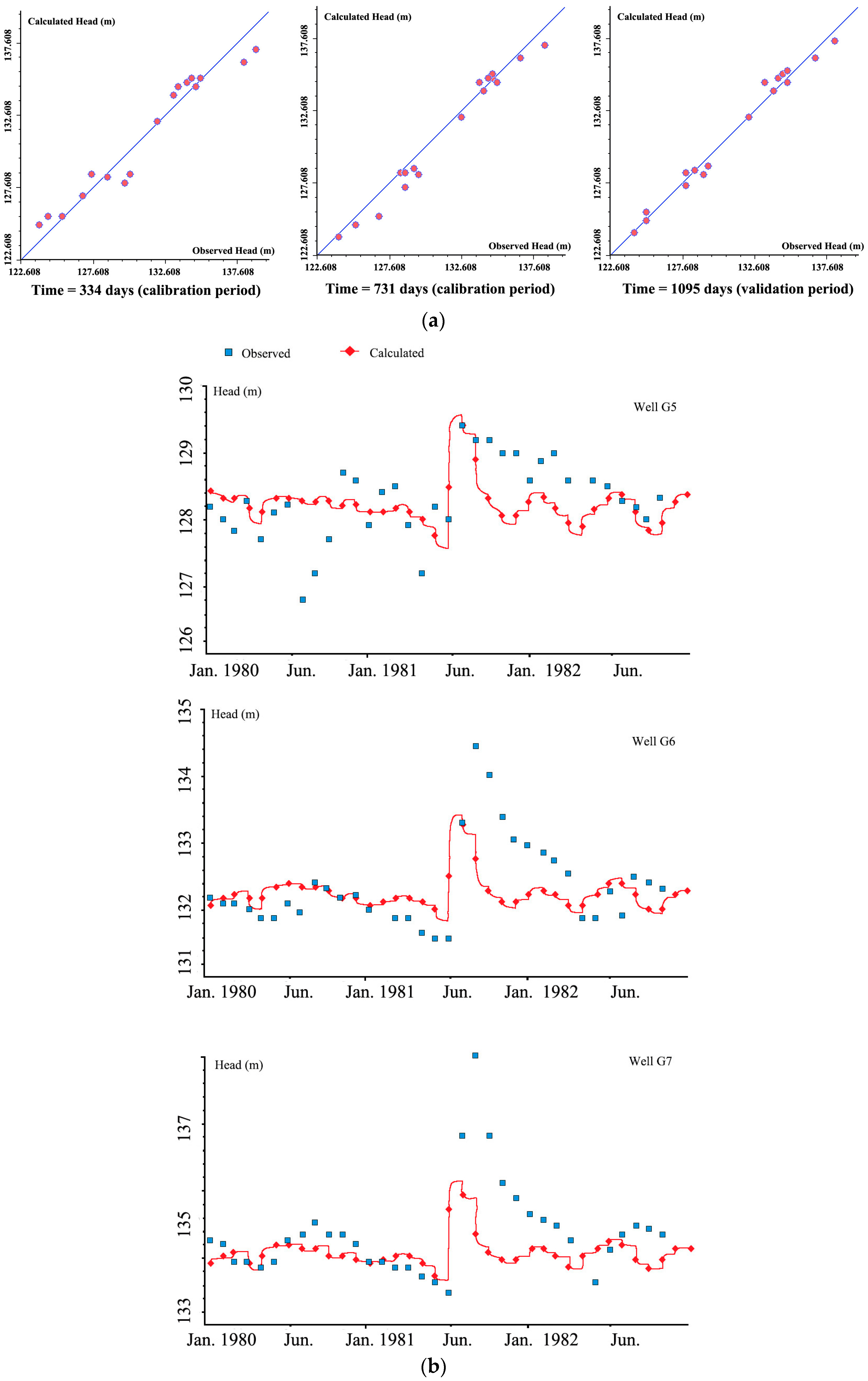
3.2. Establishment of the Groundwater Flow Model
- The terrain to the west of the study area is higher, and groundwater flows here from west to east, which makes the discharge of the upper reaches of the river in the study area larger.
- The aquifer materials of the upper reaches of the river in the study area were mostly boulders and gravels, with high permeability, thus resulting in high hydraulic conductivity. Therefore, larger changes in drawdown can occur as groundwater in this area is more easily exploited.
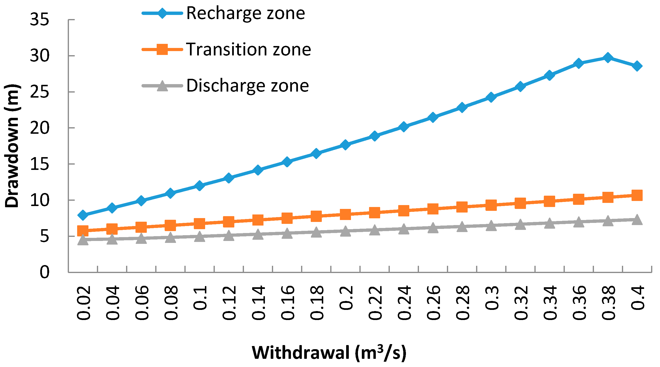
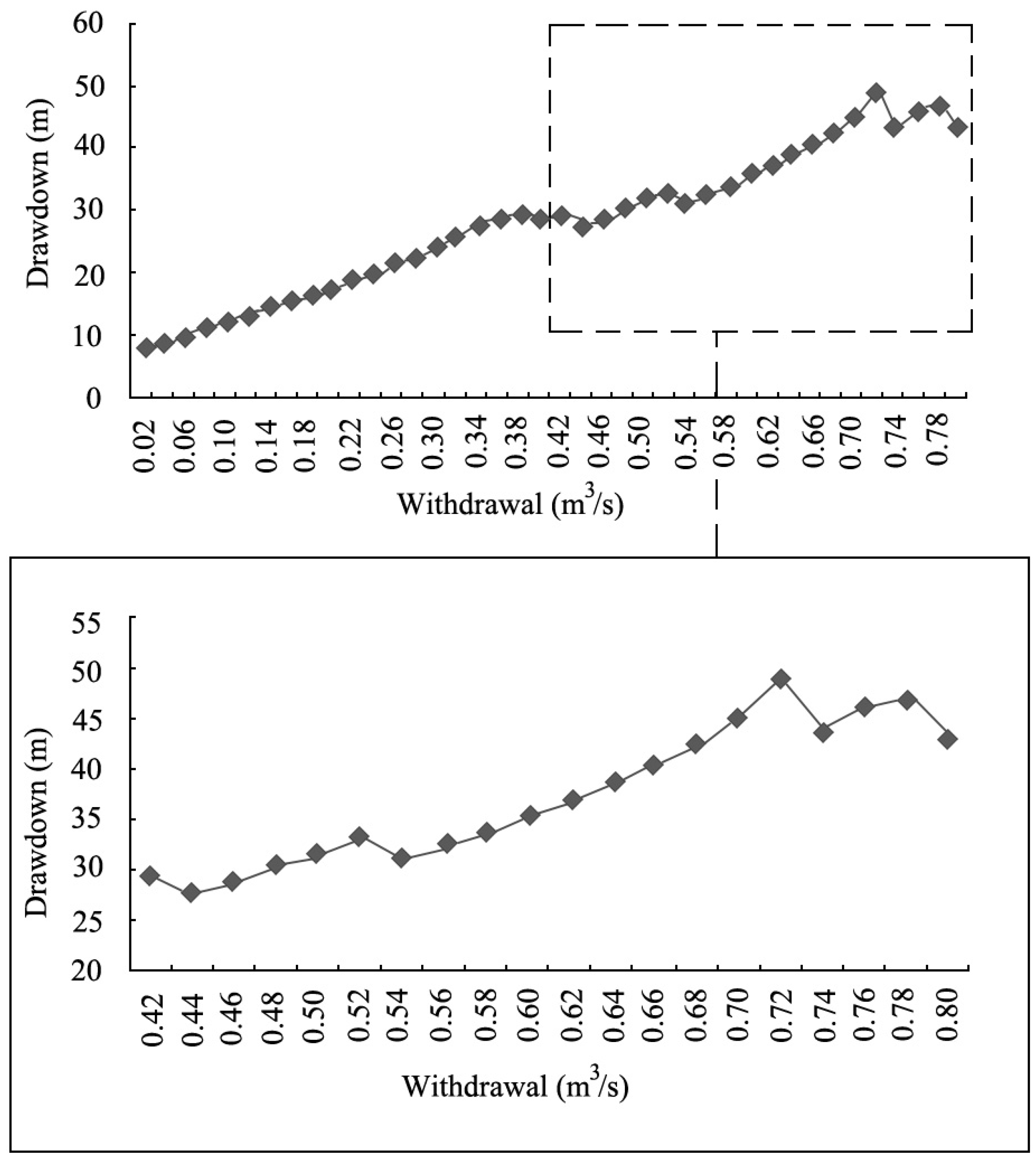
3.3. Drawdown Changes under Different Cases
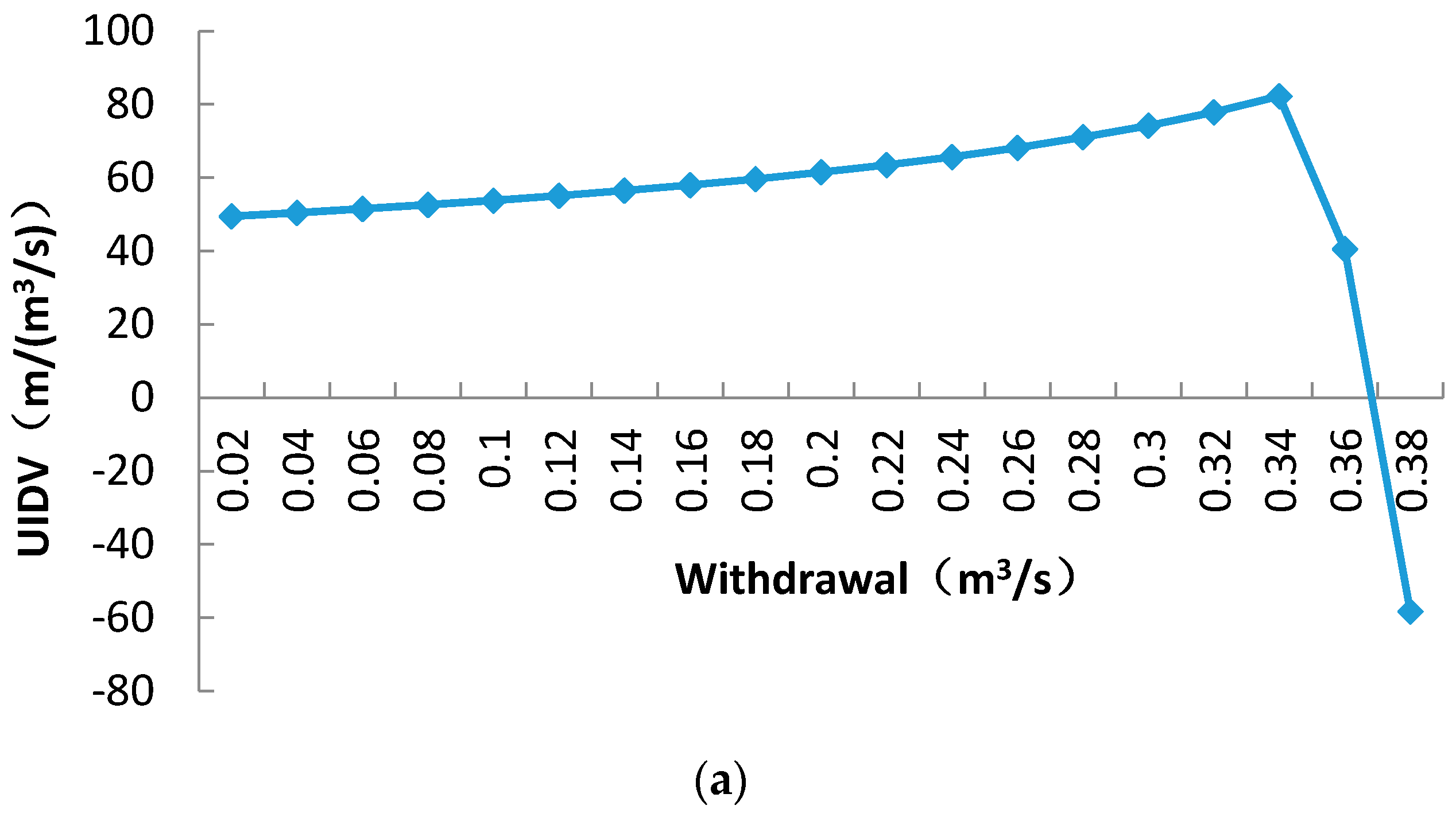
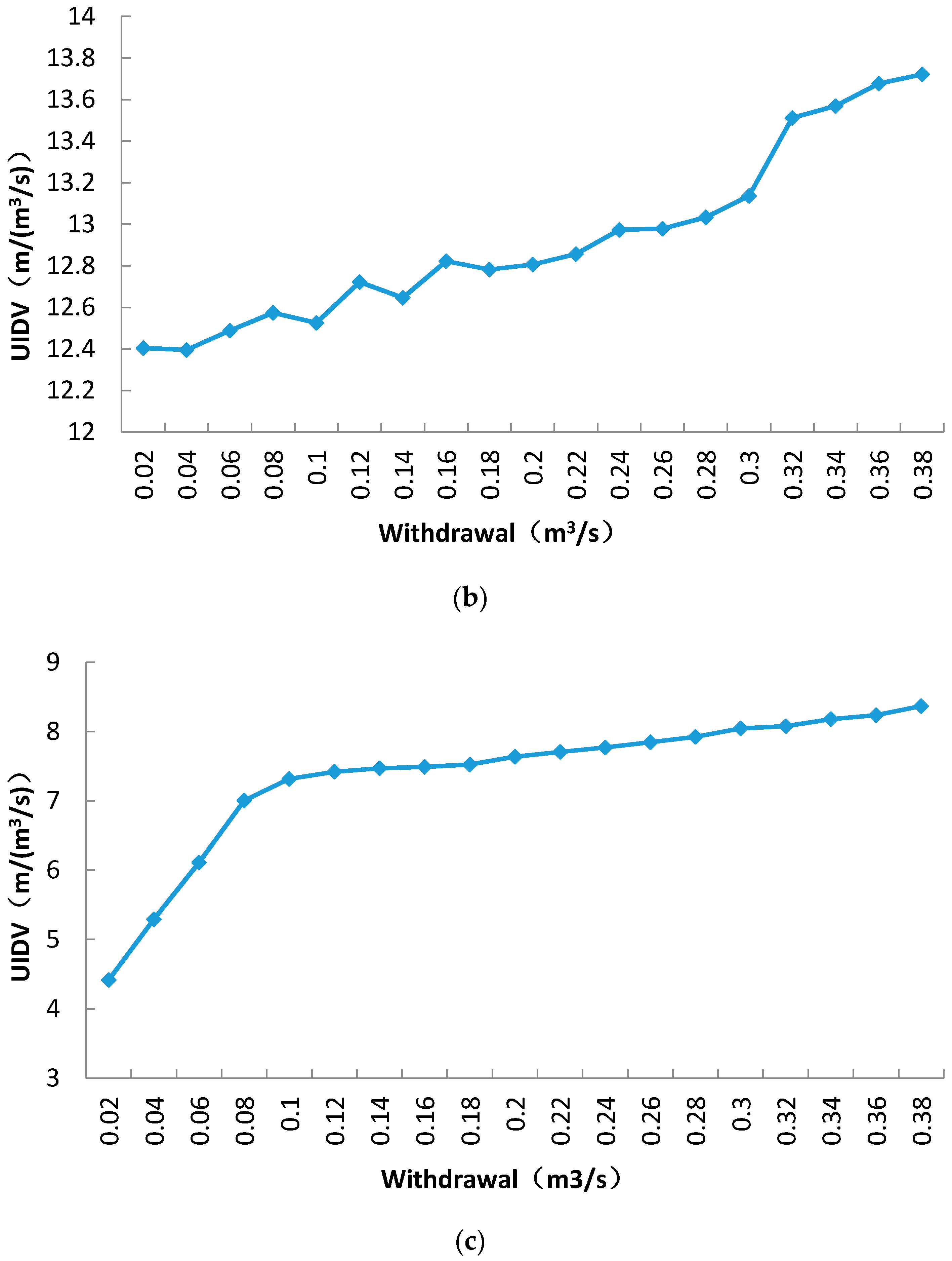
3.4. Unit Increased Drawdown Value (UIDV) Changes under Different Cases
- In the recharge zone case, UIDV increased with increases in the withdrawal, and the values ranged from 49.4 m/(m3/s) to 82.2 m/(m3/s) (Figure 13a). This trend continued until the 19th and 20th scenario, where UIDV dropped sharply and displayed negative values. These results suggest that with the trend of increasing withdrawal, the groundwater level decreased and presented an upward decreasing trend until the moment when the groundwater level fell below the confining bed of the aquifer (which is consistent with the drawdown conditions). This implies that when the withdrawal forces the groundwater level to be lower than the confining bed of the aquifer, neither drawdown nor UIDV were calculated properly by the model. Moreover, according to the familiar trend between UIDV and drawdown conditions, the data imply that UIDV expresses the same physical meaning as the drawdown to some extent.
- In the transition zone case, UIDV ranged from 12.4 m/(m3/s) to 13.7 m/(m3/s), as shown in Figure 13b. We could assume from the modeling results that the UIDV in the transition zone would always be smaller than that in the recharge zone, but obviously the change in UIDV in the transition zone is not monotonic according to the model.
- In the discharge zone case, UIDV ranged from 4.41 m/(m3/s) to 8.37 m/(m3/s) (Figure 13c). The value of UIDV in the discharge zone was the smallest and most stable, with a monotonically increasing trend, which was similar to the trend for the drawdown conditions. However, a key difference between UIDV and drawdown was as follows: UIDV reflects the increasing rate of drawdown, and thus, the value of UIDV could better reflect the situation of drawdown changes.
3.5. Results for the Pumping Well Location Selection
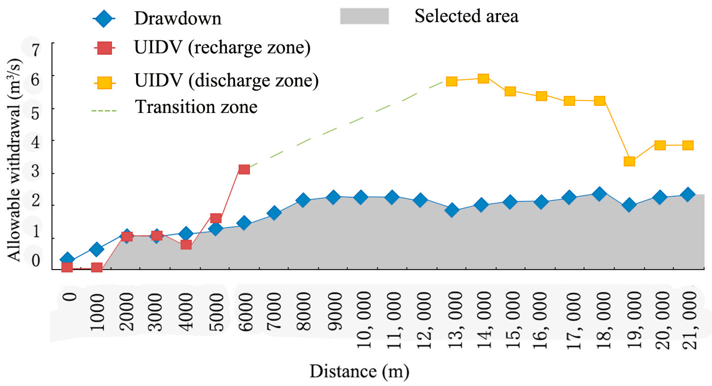
- To maximize exploitation, wells should be set in the area 18 km from the upstream reaches, and the pumping rates should not exceed 2.44 m3/s. This area was classified as the river discharge zone. Due to the lower elevation, local groundwater could also be recharged from upstream. Drawdown in this zone changes slowly and steadily.
- To minimize costs, wells should be set in the area with a distance of 2000 m from the upstream reaches of the Qin River, and withdrawal should not exceed 1.07 m3/s. This area is known as the river recharge zone. Because of the higher terrain in the study area, the aquifer is underdeveloped. Drawdown changes will thus likely be larger for extraction in this area. If wells are located in the area less than 2 km from the upstream reaches, this will lead to excessive drawdown even at low pumping rates.
- In the area at a distance between 7000 and 12,000 m from the upstream area (this area belongs to the transition zone), the relationships between groundwater and surface water were unstable, and this caused the UIDV to be highly variable. During the pumping scenarios, the trend of increasing drawdown per unit withdrawal could not be estimated, and therefore, this paper does not consider the viability of locating wells in this area.
4. Summary and Conclusions
- A numerical groundwater model was built to represent a particular study area, the Qinbei Power Plant well field. Calibration and validation of the model were performed, and the results demonstrated the reliability of this model in simulating practical problems. Based on a ten-year numerical model simulation that only considered the withdrawal of the aquifer from existing irrigation wells, drawdown for the existing withdrawal in the recharge zone and transition zone were found to be larger than in the discharge zone.
- Three cases of pumping well locations (recharge zone, transition zone, and discharge zone) were evaluated. Each case was simulated by using 20 different scenarios (with different withdrawal values) to calculate the associated drawdown. The results showed that with the same extraction volume, locating the well field in the recharge zone will produce the maximum drawdown. The well field in the transition zone had the second largest drawdown, while extraction from the discharge zone showed the minimum drawdown. Among the cases evaluated, if the groundwater level is lower than the confining bed of the aquifer, the calculated drawdown does not change monotonously with the extraction. These results indicate that groundwater recharge cannot be completely reliant on the river as a source, even though the river water level is higher than the groundwater level.
- The concept of the UIDV was introduced. Based on the drawdown results calculated in this study, UIDVs for the three cases were presented. The results showed that for the same extraction volume, well fields in the recharge zone, transition zone, and discharge zone produced the maximum, moderate, and minimum UIDVs, respectively. These results also showed that the calculated value of UIDV produced trends that were similar to drawdown, and further, that the zone of larger drawdown is likely to occur where there is a larger increasing rate of drawdown when extraction is increased by a unit value. Thus, the UIDV was useful for revealing the uncontrollability of excessive drawdown. According to the familiar trend between UIDV and drawdown conditions, the data imply that UIDV expresses the same physical meaning as the drawdown to some extent. However, a key difference between UIDV and drawdown was that UIDV reflects the increasing rate of drawdown, and thus, the value of UIDV could better reflect the situation of drawdown changes.
- The selection of a well field location was done based on the results of the allowable withdrawal evaluation. For maximum exploitation, wells should be in the area 18 km from the upstream reaches, and the allowable withdrawal should not exceed 2.44 m3/s. For a program with minimum costs, wells should be in the area at a distance of 2000 m from the upstream reaches, with the allowable withdrawal not exceeding 1.07 m3/s. In the area with a distance between 7000 and 12,000 m from the upstream reaches, the relationships between groundwater and surface water were unstable, and we considered this area as an unsuitable location for a well field. The aquifer of study area, the Qinbei Power Plant, belongs to an unconfined aquifer consisting of porous media, which is a ubiquitous type around China and even all over the world. Based on the representativeness of the study area, this proposed method can be applied to other sites in China as well as in regions outside of China where there are similar issues about jointly managing groundwater and surface water resources.
Acknowledgments
Author Contributions
Conflicts of Interest
References
- Qiu, S.; Liang, X.; Xiao, C.; Huang, H.; Fang, Z.; Lv, F. Numerical simulation of groundwater flow in a river valley basin in Jilin Urban area, China. Water 2015, 7, 5768–5787. [Google Scholar] [CrossRef]
- Parsons, M.C.; Hancock, T.C.; Kulongoski, J.T.; Belitz, K. Status of Groundwater Quality in the Borrego Valley, Central Desert, and Low-Use Basins of the Mojave and Sonoran Deserts Study Unit, 2008–2010: California GAMA Priority Basin Project; U.S. Geological Survey: Sacramento, CA, USA, 2014.
- Sophocleous, M. From safe yield to sustainable development of water resources-the Kansas experience. J. Hydrol. 2000, 235, 27–43. [Google Scholar] [CrossRef]
- Lerner, D.N. Predicting pumping water levels in single and multiple wells using regional groundwater models. J. Hydrol. 1989, 105, 39–55. [Google Scholar] [CrossRef]
- Székely, F. Pumping test data analysis in wells with multiple or long screens. J. Hydrol. 1992, 132, 137–516. [Google Scholar] [CrossRef]
- Jiao, J.J.; Rushton, K.R. Sensitivity of drawdown to parameters and its influence on parameter estimation for pumping tests in large-diameter wells. Ground Water 1995, 33, 794–800. [Google Scholar] [CrossRef]
- Singh, V.S. Well storage effect during pumping tests in an aquifer of low permeability. Hydrol. Sci. J. 2000, 45, 589–594. [Google Scholar] [CrossRef]
- Singh, S.K. Aquifer parameters from drawdowns in large-diameter wells: Unsteady pumping. J. Hydrol. Eng. 2008, 13, 636–640. [Google Scholar] [CrossRef]
- Székely, F. Evaluation of pumping induced flow in observation wells during aquifer testing. Ground Water 2012, 51, 762–767. [Google Scholar] [CrossRef] [PubMed]
- Saeed, M.M.; Ashraf, M.; Asghar, M.N. Hydraulic and hydro-salinity behavior of skimming wells under different pumping regimes. Agric. Water Manag. 2003, 61, 163–177. [Google Scholar] [CrossRef]
- Rao, S.V.; Manju, S. Optimal pumping locations of skimming wells. Hydrol. Sci. J. 2007, 52, 352–361. [Google Scholar] [CrossRef]
- Zhao, W.Q.; Pang, D.H.; Zhang, Y.S.; Leng, X.S. Location selection of deepwater relief wells in South China Sea. Pet. Explor. Dev. 2016, 43, 315–319. [Google Scholar] [CrossRef]
- Salmachi, A.; Bonyadi, M.R.; Sayyafzadeh, M.; Haghighi, M. Identification of potential locations for well placement in developed coalbed methane reservoirs. Int. J. Coal Geol. 2014, 131, 250–262. [Google Scholar] [CrossRef]
- Rodrigues, H.W.L.; Prata, B.A.; Bonates, T.O. Integrated optimization model for location and sizing of offshore platforms and location of oil wells. J. Pet. Sci. Eng. 2016. [Google Scholar] [CrossRef]
- Boyce, S.E.; Nishikawa, T.; Yeh, W.W. Reduced order modeling of the Newton formulation of MODFLOW to solve unconfined groundwater flow. Adv. Water Resour. 2015, 83, 250–262. [Google Scholar] [CrossRef]
- Ou, G.; Chen, X.H.; Kilic, A.; Bartelt-Hunt, S.; Li, Y.S.; Samal, A. Development of a cross-section based streamflow routing package for MODFLOW. Environ. Model. Softw. 2013, 50, 132–143. [Google Scholar] [CrossRef]
- Ou, G.; Li, R.; Pun, M.; Osborn, C.; Bradley, J.; Schneider, J.; Chen, X.H. A MODFLOW package to linearize stream depletion analysis. J. Hydrol. 2015, 532, 9–15. [Google Scholar] [CrossRef]
- Guzman, J.A.; Moriasi, D.N.; Fowda, P.H.; Steiner, J.L.; Starks, P.J.; Arnold, J.G.; Srinivasan, R. A model integration framework for linking SWAT and MODFLOW. Environ. Model. Softw. 2015, 73, 103–116. [Google Scholar] [CrossRef]
- McDonald, M.G.; Harbauch, A.W. A Modular Three-Dimensional Finite-Difference Ground-Water Flow Model; U.S. Geological Survey: Reston, VA, USA, 1988; Chapter A1.
- Iyalomheb, F.; Rizzia, J.; Pasinia, S.; Torresana, S.; Crittoa, A.; Marcominia, A. Regional Risk Assessment for climate change impacts on coastal aquifers. Sci. Total Environ. 2015, 537, 100–114. [Google Scholar] [CrossRef] [PubMed]
- Goderniauxa, P.; Brouyèreb, S.; Wildemeerschd, S.; Therrienc, R.; Dassarguesb, A. Uncertainty of climate change impact on groundwater reserves—Application to a chalk aquifer. J. Hydrol. 2015, 528, 108–121. [Google Scholar] [CrossRef]
- Bolster, C.; Genereux, D.; Saiers, J. Determination of specific yield for a lime-stone aquifer from a canal drawdown test. Ground Water 2001, 39, 768–777. [Google Scholar] [CrossRef] [PubMed]
- Saiers, E.J.; Genereux, D.P.; Bolster, C.H. Influence of calibration methodology on ground water flow predictions. Ground Water 2004, 42, 32–44. [Google Scholar] [CrossRef] [PubMed]
- Hughes, J.D.; Langevin, C.D.; Chartier, K.L.; White, J.T. Documentation of the Surface-Water Routing (SWR1) Process for Modeling Surface-Water Flow with the U.S. Geological Survey Modular Groundwater Model (MODFLOW-2005): U.S. Geological Survey Techniques and Methods; U.S. Geological Survey: Tampa, FL, USA, 2012; pp. A6–A40.
- Harbaugh, A.W.; Banta, E.R.; Hill, M.C.; McDonald, M.G. MODFLOW-2000, the U.S. Geological Survey Modular Ground-Water Model—User Guide to Modularization Concepts and the Ground-Water Flow Process; Open-File Report; U.S. Geological Survey: Reston, VA, USA, 2000.
- Huo, C.R.; Wang, Y.L. Hydrogeology; Water Power Press: Beijing, China, 1988. [Google Scholar]
- Zhang, M.; Yuan, H. The PauTa criterion and rejecting the abnormal value. J. Zhengzhou Univ. Technol. 1997, 18, 84–88. [Google Scholar]
- Cardenas, M.B.; Zlotnik, V.A. Three-dimensional model of modern channel bend deposits. Water Resour. Res. 2003, 39, 1141. [Google Scholar] [CrossRef]
- Chen, X.H. Statistical and geostatistical features of streambed hydraulic conductivities in the Platte River, Nebraska. Environ. Geol. 2005, 48, 693–701. [Google Scholar] [CrossRef]


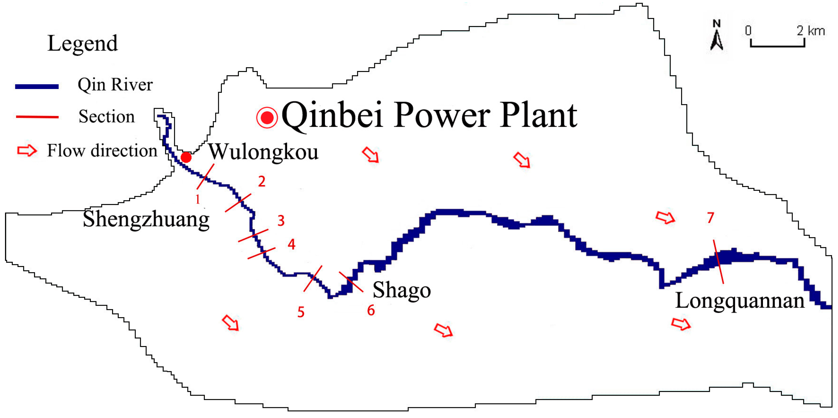
| Section | Interval Distance | Recharge Item | Discharge Item | Amount of Infiltration |
|---|---|---|---|---|
| No. 1 (Shengzhuang)–No. 6 (Shagou) | 7.80 km | Qin River | Aquifer | 0.35 m3/s |
| No. 6 (Shagou)–No. 7 (Longquannan) | 14.40 km | Aquifer | Qin River | 2.09 m3/s |
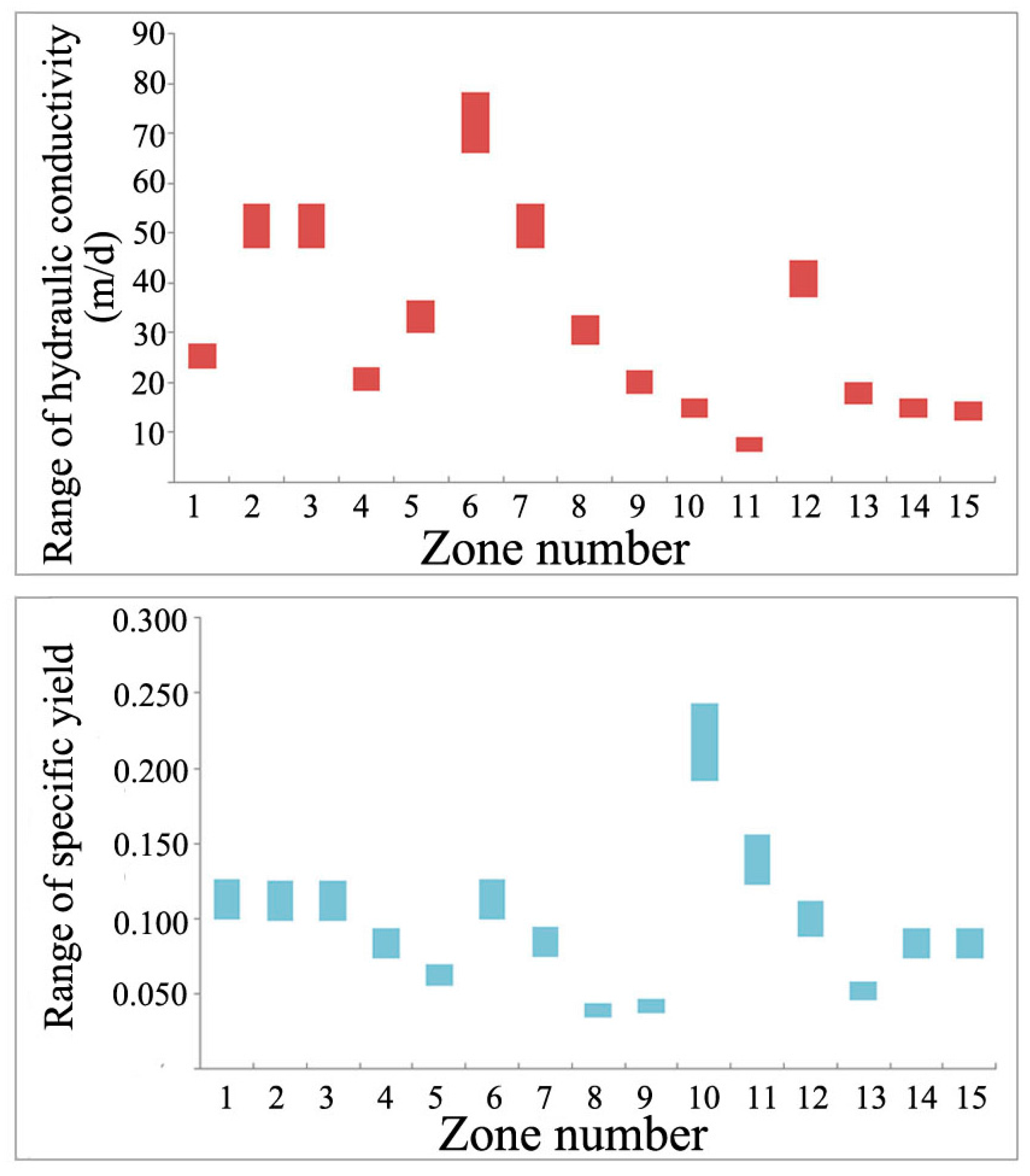
| Zone | 1 | 2 | 3 | 4 | 5 | 6 | 7 | 8 |
|---|---|---|---|---|---|---|---|---|
| K (m/d) | 25 | 50 | 50 | 20.5 | 32.6 | 70 | 50 | 30 |
| Zone | 9 | 10 | 11 | 12 | 13 | 14 | 15 | – |
| K (m/d) | 20 | 15 | 8 | 39.9 | 17.9 | 15 | 14.5 | – |
| Zone | 1 | 2 | 3 | 4 | 5 | 6 | 7 | 8 |
| μ | 0.113 | 0.112 | 0.112 | 0.084 | 0.062 | 0.113 | 0.085 | 0.039 |
| Zone | 9 | 10 | 11 | 12 | 13 | 14 | 15 | – |
| μ | 0.042 | 0.217 | 0.139 | 0.1 | 0.052 | 0.084 | 0.084 | – |
© 2016 by the authors; licensee MDPI, Basel, Switzerland. This article is an open access article distributed under the terms and conditions of the Creative Commons Attribution (CC-BY) license (http://creativecommons.org/licenses/by/4.0/).
Share and Cite
Chen, S.; Shu, L.; Lu, C. A New Method for Evaluating Riverside Well Locations Based on Allowable Withdrawal. Water 2016, 8, 412. https://doi.org/10.3390/w8090412
Chen S, Shu L, Lu C. A New Method for Evaluating Riverside Well Locations Based on Allowable Withdrawal. Water. 2016; 8(9):412. https://doi.org/10.3390/w8090412
Chicago/Turabian StyleChen, Sining, Longcang Shu, and Chengpeng Lu. 2016. "A New Method for Evaluating Riverside Well Locations Based on Allowable Withdrawal" Water 8, no. 9: 412. https://doi.org/10.3390/w8090412