1. Introduction
Inland navigation is clearly one of the most environment-friendly manners of transportation, however, it can also have negative effects. The direct contact with the propellers may cause mechanical damage to aquatic animals [
1] and plants. Oil and fuel contaminations may affect the water quality [
2]. Canals built to connect river systems result in removing biogeographical boundaries, which may lead to the degradation of biodiversity by the invasion of non-native species [
3,
4].
Inland navigation also has a direct physical effect on aquatic habitats through the alteration of the local hydraulic regime, i.e., the generation of currents and ship-induced waves. These waves may cause the resuspension of sediment in shallow water areas [
5,
6], which reduces the availability of light for the growth of phytoplankton [
7] and biofilms in particular and also affect the hunting success of visually orientated fishes [
8].
Studies have shown that the local increase of bed shear stress—generated by ship induced waves—has serious impact on fish eggs, juvenile fish and macroinvertebrates living in, on or close to the river substrate. Increased shear stress can detach individuals from their natural habitats, which may even be lethal. The ecological aspects of this issue have already been investigated in several studies (e.g., [
9,
10,
11]), but thorough analyses focusing on near bed hydrodynamics and related variation of bed shear stress can hardly be found.
Recent studies conducted in a short reach of the Austrian Danube showed that characteristics of the complex wave system can be assessed based on data acquired by proper field measurements [
12]. They found that drawdown caused by vessels travelling at sub-critical speed to be the highest, however the highest and longest waves were induced by a supercritical fast catamaran and a speedboat. Another notable feature was the long duration of the wave events, which is probably explainable by the reflections between the riverbanks. Eco-hydraulic investigations estimated the drift of fish larvae by the exposing of drift nets near the shore to collect specimens being swept into the current [
13,
14]. It was found that near-bank, shallow water habitats with inhomogeneous morphology and woody debris may provide safer conditions compared to more exposed areas with gravel bed, where displacements and drifting due to ship induced waves are more likely. Moreover, the effects of different hydrological conditions were also investigated, which might mean a first step towards durability-based eco-hydraulic investigations in connection with the effects of inland navigation.
Besides the experimental studies a few examples can be found on the numerical modeling of ship induced waves focusing on the effects on the riverbed [
15,
16]. These studies focused on the influence of waves on sediment resuspension and highlighted the connection between maximal suspended particle matter (SPM) concentrations and the speed of the ships, and also showed the dependency of sediment concentration on the position of the ships. According to the authors’ knowledge there are no studies yet which focus on the fine scale simulation of ship induced waves at the riverbank in terms of wave velocities, wave breaking and related bed shear stress.
The main goal of this study is to introduce a methodology, using field observations and numerical methods, for the quantification of the influence of ship induced waves on the riverbank. As to the field measurements acoustic (Acoustic Doppler Velocimetry (ADV)) and image based (Large Scale Particle Image Velocimetry (LSPIV)) techniques are proposed and for the computational modeling a computational fluid dynamics (CFD) model is applied. In order to prove the future applicability of the method, the study makes an attempt to reveal the answers to the following issues:
Is there a significant spatial variability (perpendicular with the bank) of wave generated near-bed velocities and bed shear stress in the littoral zone?
Which is the most suitable formula to estimate local bed shear stress in rivers when waves present?
Can the LSPIV method be an alternative way to measure wave propagation in zones where acoustic methods are not feasible anymore (e.g., at temporally dry areas)?
Can a numerical tool provide such detailed information as the field measurement methods for situations where no field data collection is feasible (e.g., to analyze the effect of planned measures)?
Compared to previous studies a significant step forward using ADV for near-bed velocity measurements is the parallel application of three devices to reveal the spatial variation of characteristic velocities and bed shear stress values towards the riverbank. Besides the acoustic methods, we present the application of LSPIV of the water surface. LSPIV is used to estimate the propagation velocity of the breaking waves at the bank in zones which are only temporally wetted due to the waves. The local bed shear stress is estimated based on the velocity measurements, testing several formulas, some of which take into account the turbulent effects and others the wave effects. Besides the field data analysis, an attempt is made to simulate ship generated waves with computational fluid dynamics (CFD). The open-source numerical model REEF3D is employed, which is capable to calculate complex free surface flows and waves [
17,
18]. As a sample application we analyze the hydrodynamic characteristics of waves induced by different ship types in the littoral zone of a study section of the Hungarian Danube.
2. Materials and Methods
2.1. Study Site
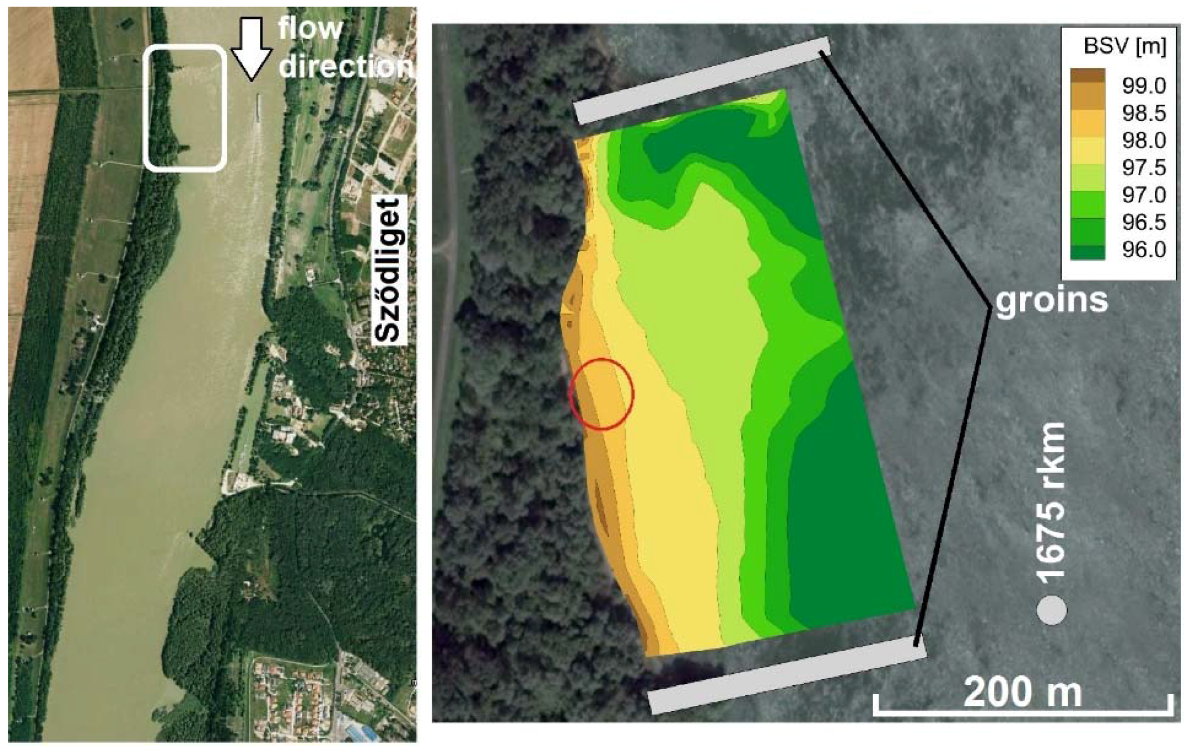
The study area is located in a free flowing reach of River Danube at river kilometer (rkm) 1675 close to the town of Sződliget, at the right bank of the main channel. Actually this is the left branch of the Danube divided by the 31 km long Szentendrei Island. Two-thirds of the total discharge flows in this branch of the river, with an annual mean of 1300 m3·s−1; consequently, this arm is used as the navigational channel. The mean flow depth is around 5 m, and the river width is 400 m.
In order to ensure the adequate navigational depth in the river, two pairs of groins were built in the area. The field measurements were performed between the upstream pair of groins, at the near bank zone (
Figure 1). The riverbank can be characterized with a slope of 1:7. The bed material is sand with a mean diameter of 0.2 mm. At low flows, due to the groins, the flow velocities at the study zone are quite low and the bank is, in fact, impacted chiefly by ship generated waves.
2.2. Field Data Collection
In order to understand the hydrodynamic features and to assess the spatio-temporal variability of the bed shear stress caused by the waves, high time resolution, three-dimensional near bed velocity time series were collected. Three ADVs (2 × Nortek Vectrino and a Nortek Vector) were deployed during the field campaign using a sampling frequency of 16 Hz. The instruments were set up at a regular interval along a line perpendicular to the riverbank, at distances 1.8 m, 3.8 m and 5.8 m from the bank, respectively. The ADVs were carefully fixed to sample the boundary layer right above the riverbed at a distance of approximately 1 cm. The velocity sampling by the devices was synchronized using a separate unit for this purpose. Besides the velocity measurements, the ADV located farthest from the riverbank detected the pressure fluctuations as well.
The measurement setup was completed with a Full HD video camera (GoPro Hero 4, GoPro, Inc., San Mateo, CA, USA) mounted on fixed frame at the riverbank, in the zone of the breaking waves. The camera had wide-angle lens making it suitable to record the approaching and breaking waves. The setup provided a usable area of approximately 5 m2. The recorded videos were later analyzed with LSPIV.
During the one-day-long measurement campaign, the flow discharge was 1750 m
3·s
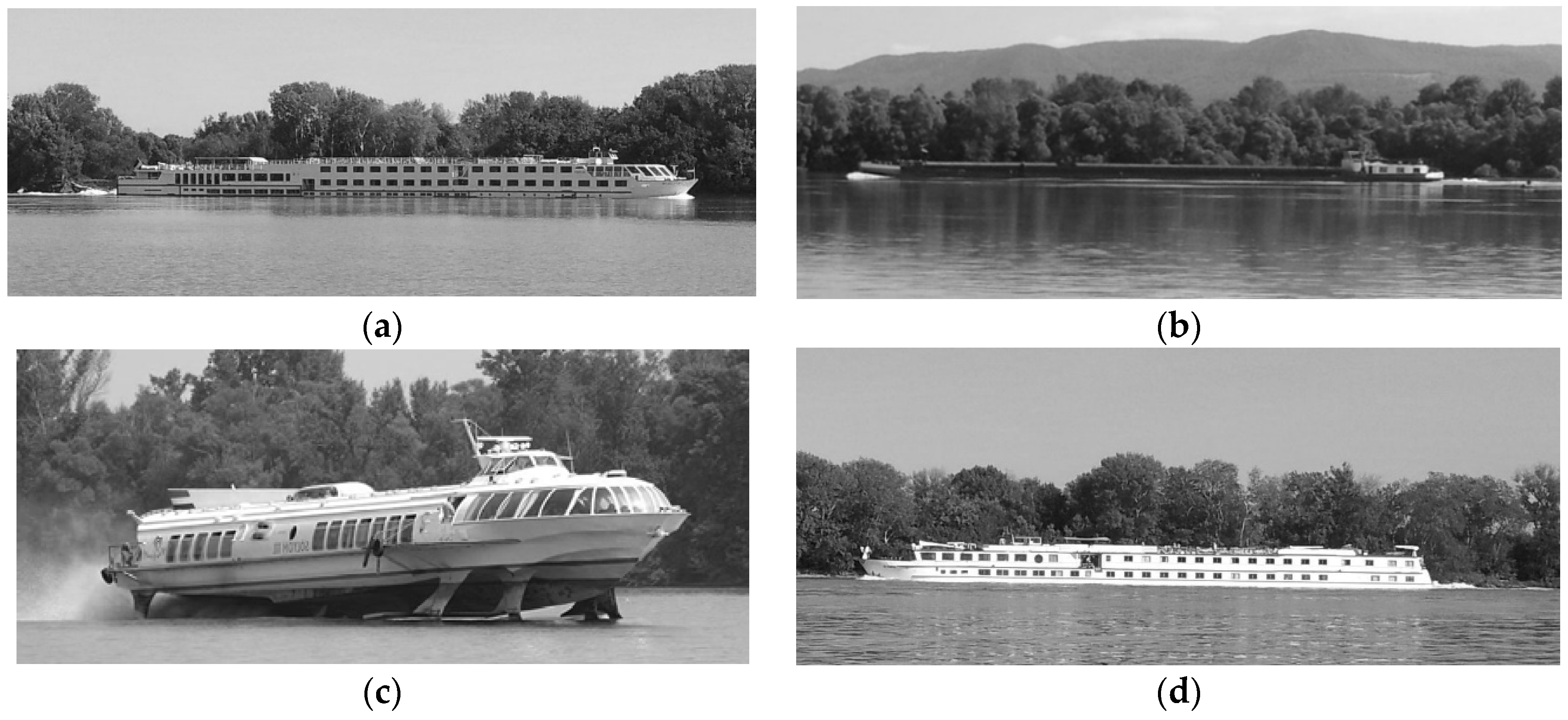
−1, somewhat higher than the annual mean. However, the crests of the nearby groins were still emerged resulting in a very slow recirculation at the study section, and negligible flow velocities compared to the ship generated waves. During the measurements, four passenger vessels, a barge and a hydrofoil passed by, and so the hydrodynamic effects of their movement were analyzed. Due to the similarity of the results of the same vessel type, in the following, we focus on the data analysis of two passenger vessels, the barge and the hydrofoil (
Figure 2).
The most relevant data regarding the geometry and the speed of the ships are presented in
Table 1. It is noted that the present study does not aim to investigate the connections between ship and wave parameters, and the following data are only presented for the sake of completeness.
2.3. Data Analysis
2.3.1. Analysis of the Velocity Measurements
The high time resolution three-dimensional velocity series obtained by the ADV devices were used for several purposes: (i) analyze the spatial and temporal variability of wave propagation in the littoral zone; (ii) estimate wave generated bed shear stress; and (iii) provide boundary conditions for CFD modeling. The raw velocity data obtained by the ADV were synchronized and filtered. The data filtering was performed based on the quality of the signals, which can be characterized by the correlation of the signals and with the signal to noise ratio (SNR). The data filtering was conducted with the introduction of a correlation limit (70%) and a SNR limit (20 dB) recommended by [
20]. Where these conditions were not met, the data portion was cut out.
The filtered data series were used to analyze the flow field and to estimate turbulence related velocity fluctuations. In general, this can be performed with the Reynolds decomposition separating the actual velocity vector u into a time-averaged and a fluctuating u′ component.
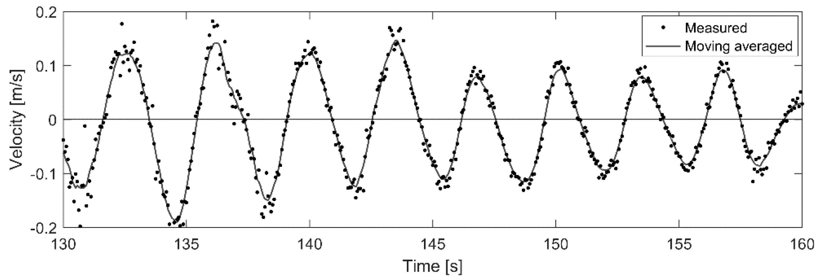
The separation of mean and turbulent components is, however, not straightforward when analyzing waves as the mean velocity is itself fluctuating with the waves at a much longer time scale than turbulence. In this case, we applied the following assumption: moving averaged velocity values were accepted as mean values, and the deviation from that was considered as turbulent fluctuation (
Figure 3). After performing a sensitivity analysis on the window size and considering the spectral range of the waves, a time window of 0.7 s was used for the central moving averaging. This window size was found to be suitable for the all the collected time series, as the bulk wave parameters (wave amplitude, frequency) derived from the smoothed and the raw data series matched this way [
21].
Using the Reynolds decomposed velocity time series an attempt was made to quantify the bed shear stress related to turbulence. In riverine conditions, there are different methods available to perform these calculations based on turbulence related parameters, however, wave induced bed shear stress could be derived from wave related parameters as well.
In the case of three-dimensional velocity measurements, all components have to be decomposed (
u is in the direction of the mean flow,
v is perpendicular to u in the horizontal plane and
w is the upward vertical component). The relationship between the mean of the product of fluctuating components and the bed shear velocity is the following [
22]:
where
κ is the von Kármán constant (≈0.4),
ν is the kinematic viscosity of the water (≈10
−6 m
2·s
−1),
Re is the Reynolds number and
is the bottom friction velocity. In the case of turbulent flows, the Reynolds number
, thus
and
τb is the bed shear stress
therefore
where
ρ is the density of water.
It has been reported that there is a linear connection between the bed shear stress and the turbulent kinetic energy (TKE) appearing on the riverbed [
23]. The ratio between these parameters is
C1 ≈ 0.19 [
24]. The value of the TKE can be evaluated from the turbulent fluctuation of the velocity components:
therefore
There is an alternative form to estimate bed shear stress that only requires the turbulent fluctuation of the vertical velocity component (
w) [
25]:
where the constant ratio
C2 ≈ 0.9.
In the case of wave induced turbulence, however, these calculations are far from trivial, e.g., the direction of the slowly fluctuating mean flow is not unequivocal due to the spatial complexity of flow field. This is why a fourth method developed for wave bottom boundary layers was also employed in the present study. This method assumes that the effects of wave-phase averaged currents are negligible and the bed shear stress can be determined uniquely from phase-averaged wave variables. The bed shear stress is proportional to the second power of the maximum orbital velocity at the bed,
Uw [
26]:
where
fw is the Darcy-type wave friction factor [
27]:
and
A is the semi-orbital excursion determined using
Uw (average of the ten highest measured near-bed velocities from the filtered time-series) and wave period
T (averaged for every measurement period) as
2.3.2. Large Scale Particle Image Velocimetry
LSPIV is an image based velocity measurement method, which requires video records capturing the water surface to calculate two-dimensional (horizontal) velocity fields (see e.g., [
28]). The method was developed for fast, cost-efficient discharge measurements in streams and is proven to be a good alternative to conventional in situ methods [
28,
29,
30,
31,
32]. The LSPIV identifies patches and patterns on the consecutive video frames and evaluates their displacement, thus the velocity vectors can be calculated by dividing displacements with the elapsed time between two frames. The strength of the method lies in its simplicity and low computational cost: its field deployment requires a video camera, a personal computer and a water level gauge only.
The goal of using LSPIV in this study was to assess the dynamics of the breaking waves, where the acoustic methods are not applicable anymore because the permanent submergence of the device cannot be ensured due to intermittent wetting and drying. In order to employ the LSPIV algorithm, the video recordings, introduced in detail later in this paper, were first broken into a series of images, and then geometrically transformed to obtain a plane view orthogonal to the free surface. These orthorectification transformations were conducted by the freely available Fudaa-LSPIV software (version 1.4.4, IRSTEA, Villeurbanne, France) [
33] based on the reference points measured during the field measurements. The relation between world and image coordinates is
where [
i,
j] are the coordinates in the reference system of the images (in pixels), (
x,
y,
z) are the world coordinates (in meters) and [
ak,
bk,
ck] are the calibrated coefficients of the transformation (in m
−1) constant for the whole recording.
Once the images have been orthorectified, the LSPIV could be performed. After conducting a sensitivity analysis on all the LSPIV parameters, the following ones were shown to have major effect on the quality of the results and on the solution time as well, hence their proper determination was crucial.
Size of the interrogation area (IA): the area of a rectangle (pixel2) where the algorithm identifies patches and patterns.
Size of the search area (SA): the area of a rectangle in the next image frame (pixel2) where the algorithm searches for the displaced patches and patterns identified in the IA.
Time step size (δt): time step between consecutive frames considered by the algorithm. This is required to evaluate velocities from the calculated displacements.
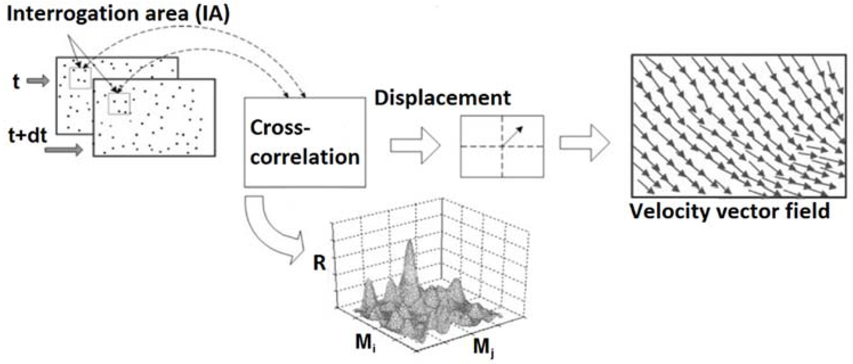
In order to perform the calculations, a grid has to be defined, where every gird point will be a center of an IA. During the calculations, the software evaluates the cross-correlation (
R) between the patterns found in every IA centered on a point
aij and the same IA centered on a point
bij in the following frame:
where
Mi and
Mj are the respective dimensions of the IA in pixels;
Aij and
Bij are the gray scale intensity of the rectangles (IA and SA, respectively); and the overbars denote averages over IA or SA. This calculation is performed for
bij included in the SA. The displacement with the highest correlation is accepted for every grid point, and then the velocity vectors are calculated. The flow chart of the algorithm is presented in
Figure 4.
The software offers different options to filter the instantaneous results. The results can be filtered with a minimal accepted correlation coefficient: if the calculated displacement has a lower R than the given minimum, the calculated velocity vector is to be removed (i.e., that grid point will be blank for the actual time interval). The other option is to set a maximal and minimal limit for the velocity components in both directions, which is an effective way to remove implausibly high velocity vectors as well.
2.4. Numerical Modeling
2.4.1. Applied Solver
The main feature of breaking waves is the complex motion of the free surface, which calls for numerical models that can resolve overturning free surfaces with multiple air-water interfaces for any vertical. For the numerical analysis, the three-dimensional numerical model REEF3D (the software name is not an abbreviation) [
34] was employed which solves the incompressible Reynolds-averaged Navier–Stokes (RANS) equations together with the continuity equation using the finite difference method. The governing RANS equations, presented here in Cartesian form, express the conservation of mass and momentum:
where
U is the velocity averaged over time;
ρ is the fluid density (considered constant here);
P is the pressure;
ν is kinematic viscosity;
νt is the turbulent eddy viscosity; and
g is the acceleration due to gravity. Indexes
i and
j refer to the Cartesian components of vector variables, and terms containing
j are implicitly summed over
j = 1...3.
The unknowns
Ui are discretized at the nodes of a regular rectangular grid. The advective term (second term of the momentum equation) is solved with the Weighted Essentially Non-Oscillatory (WENO) scheme [
35]. The stencil of the WENO scheme consists of three substencils, which are weighted according to the local smoothness of the discretized function. The scheme achieves a minimum of 3rd-order accuracy for discontinuous solutions, up to 5th-order accuracy for a smooth solution and provides robust numerical stability. Time discretization of the momentum equations is achieved with a third-order accurate total variation diminishing (TVD) Runge–Kutta scheme [
36]. The pressure term is solved with the projection method [
37] and the BiCGStab algorithm [
38] with Jacobi scaling preconditioning is used to solve the Poisson equation for the pressure. The RANS equations are closed with the two-equation k-ω turbulence model that links turbulent eddy viscosity to the Reynolds-averaged flow variables [
39].
The model employs the level set method [
40] to capture the free surface between the two phases: air and water. The method uses a signed scalar function, called level set function, to track the location of the free surface. The property of this function
is that its value gives zero on the free surface. In every point of the computational domain, the level set function gives the closest distance to the interface and the phases are distinguished by the sign as follows:
The interface moves with the water particles and its movement can be described with the advection of the level set function:
Again, the last term is summed for
j = 1 ... 3. The assumption of incompressibility and immiscibility of the fluids cause a jump in the values of the parameters at the interface, which may lead to numerical stability problems. This is avoided by smoothing the material properties in the region around the interface with a regularized Heaviside function
H(ϕ). This region is 2
ϵ thick, with
ϵ being proportional to the grid spacing
dx. In the present study, it was chosen to be
ϵ = 1.6
dx. The density and the viscosity can be written as:
and the regularized Heaviside function is defined as
2.4.2. Numerical Setup
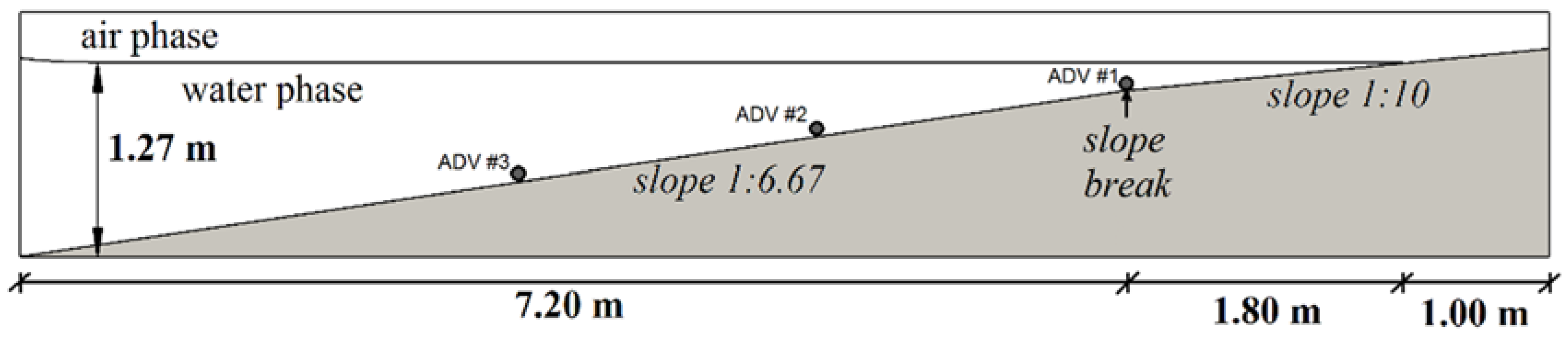
An idealized 2D slice model of the near bank region perpendicular to the bank was set up with a length of 10.0 m and a height of 1.6 m (
Figure 5). The bed profile along this perpendicular slice consisted of two sections with different slopes (1:6.67 and 1:10). An orthogonal square grid was laid over the computational domain using a uniform cell size of
dx =
dz = 10 mm. The bed geometry was discretized on this grid. The measured water depth and water levels at the points of the ADV devices from the field measurements were used to build up the geometry and to adjust the still water level. The ADV device farthest from the bank (the one equipped with the pressure sensor) was placed at 5.8 m from the bank (=still water edge). The computational domain was extended by 3.2 m towards the river, and by 1.0 m towards the initially dry land.
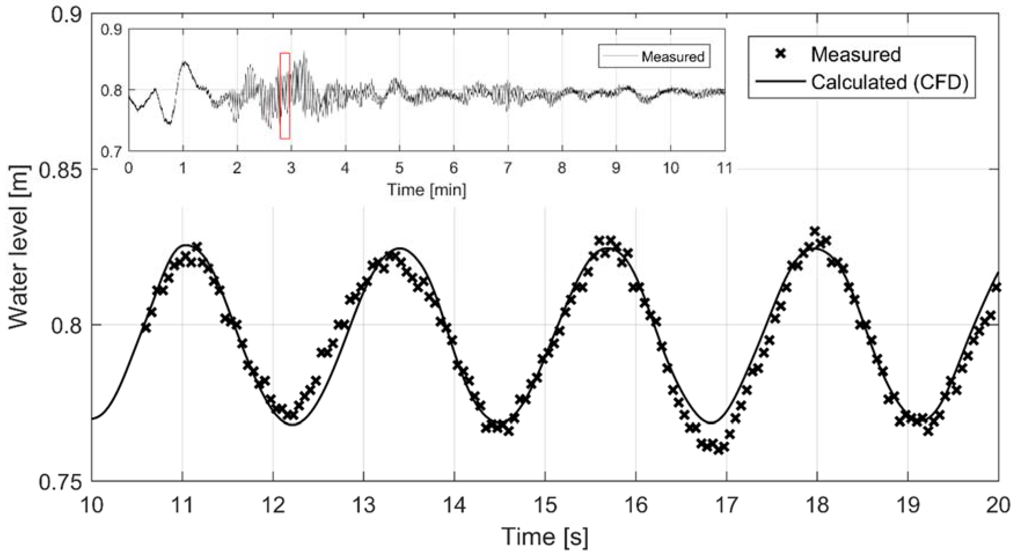
A short period of a measured wave event with fairly regular wave properties was selected for the simulations. Water level time series collected with the pressure sensor were used for defining the left boundary conditions, i.e., a wave amplitude of
A = 3.0 cm and a wave period of
T = 2.3 s was applied for wave generation according to linear wave theory.
Figure 6 presents the measured and calculated water levels in the location of the pressure gauge.
The presented section was chosen for numerical modeling because both the wave heights and the near-bed velocities were the one of the highest then, which is believed to be crucial considering near-bed habitats. It is noted that from the ecological aspect, vessel-induced drawdown may also have negative effects as the drawdown temporarily result in habitat area loss [
11], however, this study does not aim to investigate this effect.
The boundary conditions on the left end of the domain were defined based on pressure measurements taken 3.8 m closer to the bank (ADV #3), thus wave transformation might be expected. However, the comparison presented in
Figure 6 shows no notable sign of this effect, considering that deviation between the idealized and the actual wave parameters result in noticeable errors anyway.
Adaptive time stepping was used for the simulations applying the Courant–Friedrichs–Lewy (CFL) condition of 0.1. The Nikuradze roughness of the substrate was set to ks = 0.01 m based on the local d90 of the bed material.
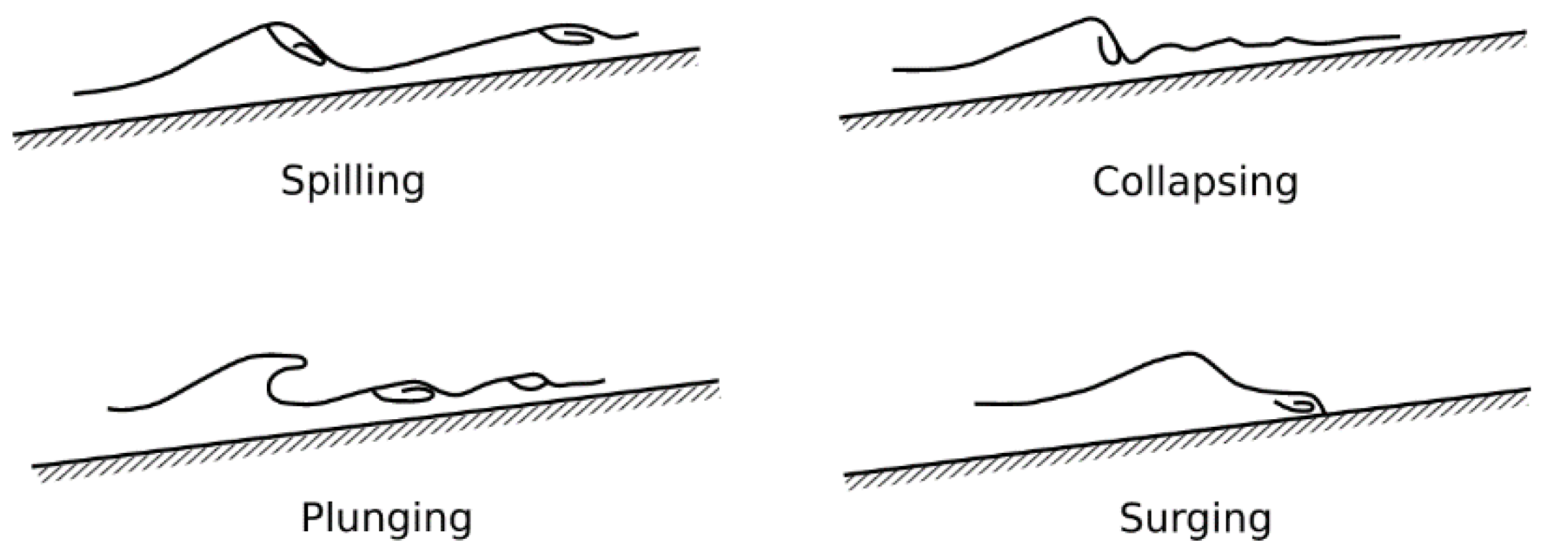
As the employed model incorporates an up-to-date free surface capturing method, the question rises whether the solver is suitably for the numerical reproduction of breaking waves. When dealing with breaking waves it has to be noted that wave height is limited by both depth and wavelength. For a given water depth and wave period, there is a maximum height limit above which the wave becomes unstable and breaks. This upper limit of wave height, called breaking wave height, is a function of the wavelength in deep water. In shallow and transitional water, it is a function of both depth and wavelength. Wave breaking is a complex phenomenon and it is one of the areas in wave mechanics that has been investigated extensively both experimentally and numerically [
41]. There are four basic types of breaking water waves: spilling, plunging, collapsing and surging (
Figure 7).
The type of wave breaking is determined by the Iribarren number (
ξ), which is a function of the slope of the shoreline (tan
α) and the wave steepness (
H/L, where
H is the wave height and
L is the wavelength):
The categorization based on the Iribarren number is the following:
3. Results
3.1. ADV Results
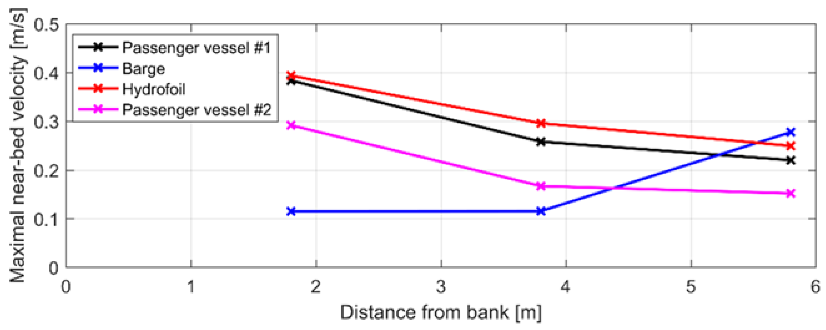
As described at the Reynolds decomposition, the measured velocity time series were filtered to remove erroneous data and moving averaged in order to eliminate turbulent fluctuations. Using the resulting dataset the maximal near bed velocity values were evaluated for each instrument (i.e., at the three points along the line perpendicular to the bank) and for each passing ship (
Figure 8).
The highest near-bed velocities resulting from ship generated waves range between 0.1 and 0.4 m/s. Compared to the mean flow velocity with no ships, which is around 0.02 m/s, this means an increase of an order of magnitude. In each case, except the barge, the highest velocities increase towards the riverbank, indicating at the same time potentially increasing bed shear stress.
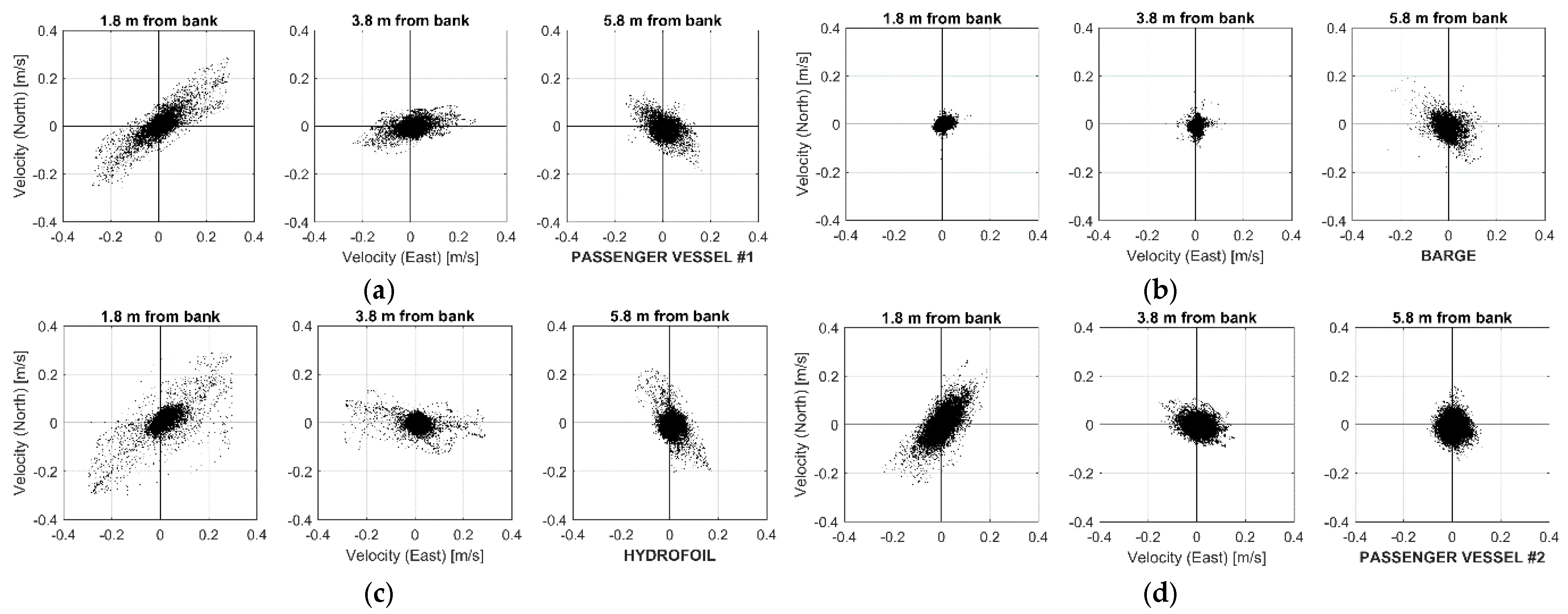
Together with the velocity magnitudes, the direction of the wave propagation towards the riverbank was also assessed. For this purpose, the velocity time series, collected during the whole measured period of each passing ship (~15 min), were post-processed. The results are shown on rose plots from the horizontal velocity component (
Figure 9).
Waves are typically approaching the riverbank in the normal direction due to wave refraction [
42]. However, in this case, the mentioned behavior cannot be observed in the figures. A significant variation of the wave direction, showing almost 90° diffraction between the measurement points farthest and closest to the bank, can be observed. This means at the same time that the direction of the approaching waves does not necessarily determine the direction of the near bed velocities. Moreover, it is noted that these directions were observed for all studied events, regardless of the ship directions (upstream, downstream). The initial orientation of the ship generated waves is determined by the ship direction, however, when the waves reach the littoral zone, the topographic steering might play a more important role. This behavior of the wave refraction, however, requires further research. Nevertheless, the results point out the surprisingly complex pattern within a small near shore area of the wave affected near bed hydrodynamics in natural conditions.
Using the estimation methods presented in
Section 2.3.1 (Equations (4) and (6)–(8)), characteristic bed shear stress values were evaluated for each ship type and for all the three measurement points. Since the first three methods derive shear stress from the mean of turbulent fluctuations, lower, time-averaged shear stress values are expected compared to the Jonsson method, which provides with a single maximal value for a whole period. From the ecological aspect, however, the latter is more relevant, since the highest shear forces result in the detachment of benthic creatures. Bed shear stress values calculated from turbulence related formulas provided (average) shear stress values between 2.25 × 10
−4 and 4.06 × 10
−1, while the Jonsson method indicated one order of magnitude higher values between 2.24 × 10
−1 and 9.51 × 10
−1 N·m
−2.
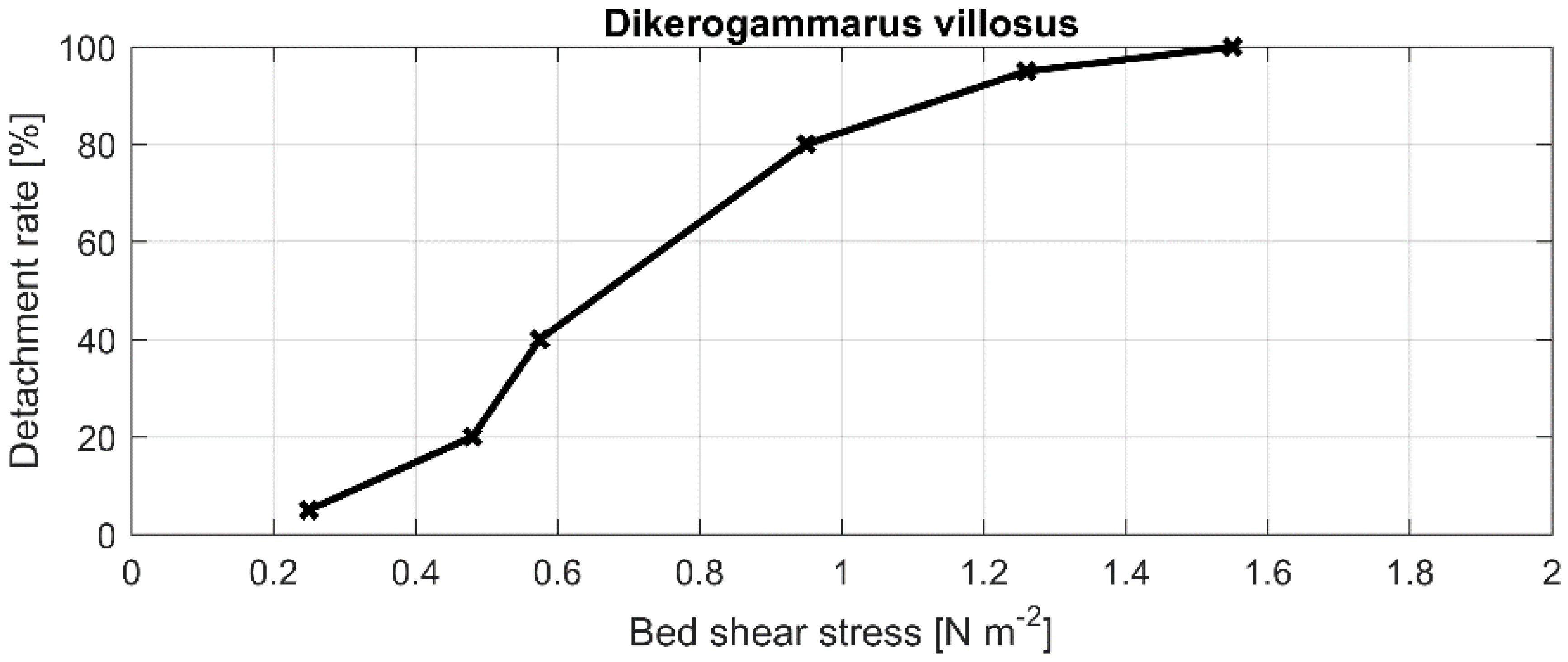
One of the main goals of the hydrodynamic assessment of ship induced waves is to provide a tool for near-bed habitat characterization. In this regard, one relevant issue is the potential detachment of the individuals caused by the wave enhanced bed shear stress. The relationship between the detachment of different macroinvertebrates from different substrates and the bed shear stress has already been investigated in both laboratory and real conditions [
9]. In the referred study, graphs were prepared which describe the relationship between the local bed shear stress and the detachment rate of different macroscale creatures. For instance, such a graph for the
Dikerogammarus villosus (a macroinvertebrate crab) is shown in
Figure 10.
In [
9], a single ADV device was deployed to evaluate the bed shear stress with the Jonsson method. In the following we perform a sample application based on the findings of that study and, as already mentioned above, we accept the applicability of the Jonsson method to estimate bed shear stress. Assuming that the study site is a suitable habitat for the
Dikerogammarus villosus the potential proportion of the detached individuals is estimated for each ship type and each measurement location.
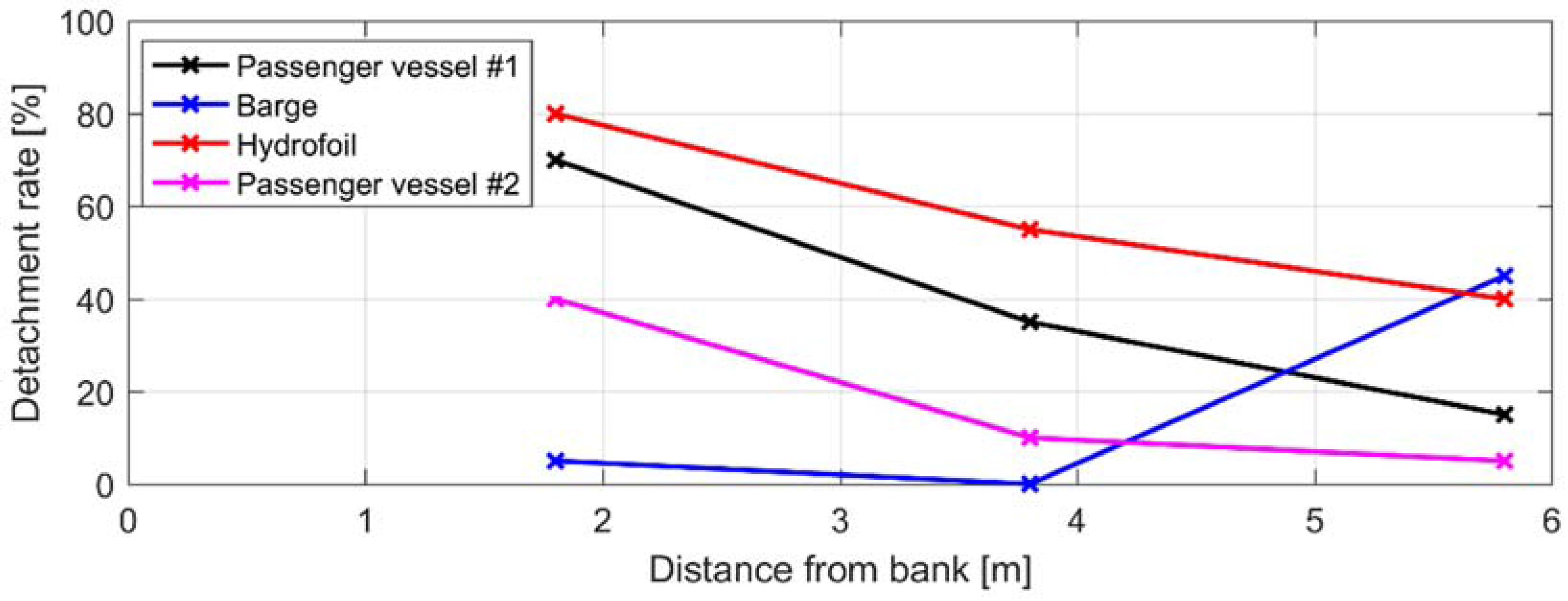
The ratio of detachment was calculated for all ship induced wave events (
Figure 11) and it is observed that the ship types typical to the studied Danube reach might have significant effects on these animals, especially in the shallowest parts of the littoral zone. Although the presented sample is not representative (four ships and three types), the results point out that significant differences between the effects of different ship types may occur, which calls for further investigations including ship related properties as well on larger samples. However, it has to be noted that the herein introduced results are rather qualitative considering that a thorough habitat study involving biologists are still to be performed to reveal locally typical species.
3.2. LSPIV Results
A section of the study area in the zone of the breaking waves was recorded using a GoPro action camera. In this area, the acoustic devices cannot be used due to the dynamically changing wet and dry zones, since the permanent submergence of the device is not ensured. The aim of this novel application of the LSPIV method was to quantify the wave propagation velocities at the bank, based on which the bed shear stress in this zone could also be estimated. As discussed in relevant LSPIV studies, one of the main prerequisites of the method is the presence of tracers on the free surface. In this case, the foam resulting from the breaking waves was detected and followed by the algorithm. It was, however, questionable if the LSPIV method is capable to quantify dynamically changing flow features, considering that the method was originally developed for discharge estimations, where the flow is quasi-steady. The following values were set for the previously mentioned parameters: image resolution = 5 mm/pixel; IA = 900 pixel
2; SA = 3250 pixel
2;
δt = 0.033 s;
Rmin = 0.75 and the computational grid had 750 (30 × 25) nodes. The calculated results for the most intense section of the wave event (highest waves) induced by passenger vessel #1 are presented in
Figure 12.
3.3. CFD Results
The 2D numerical slice model was set up as discussed in
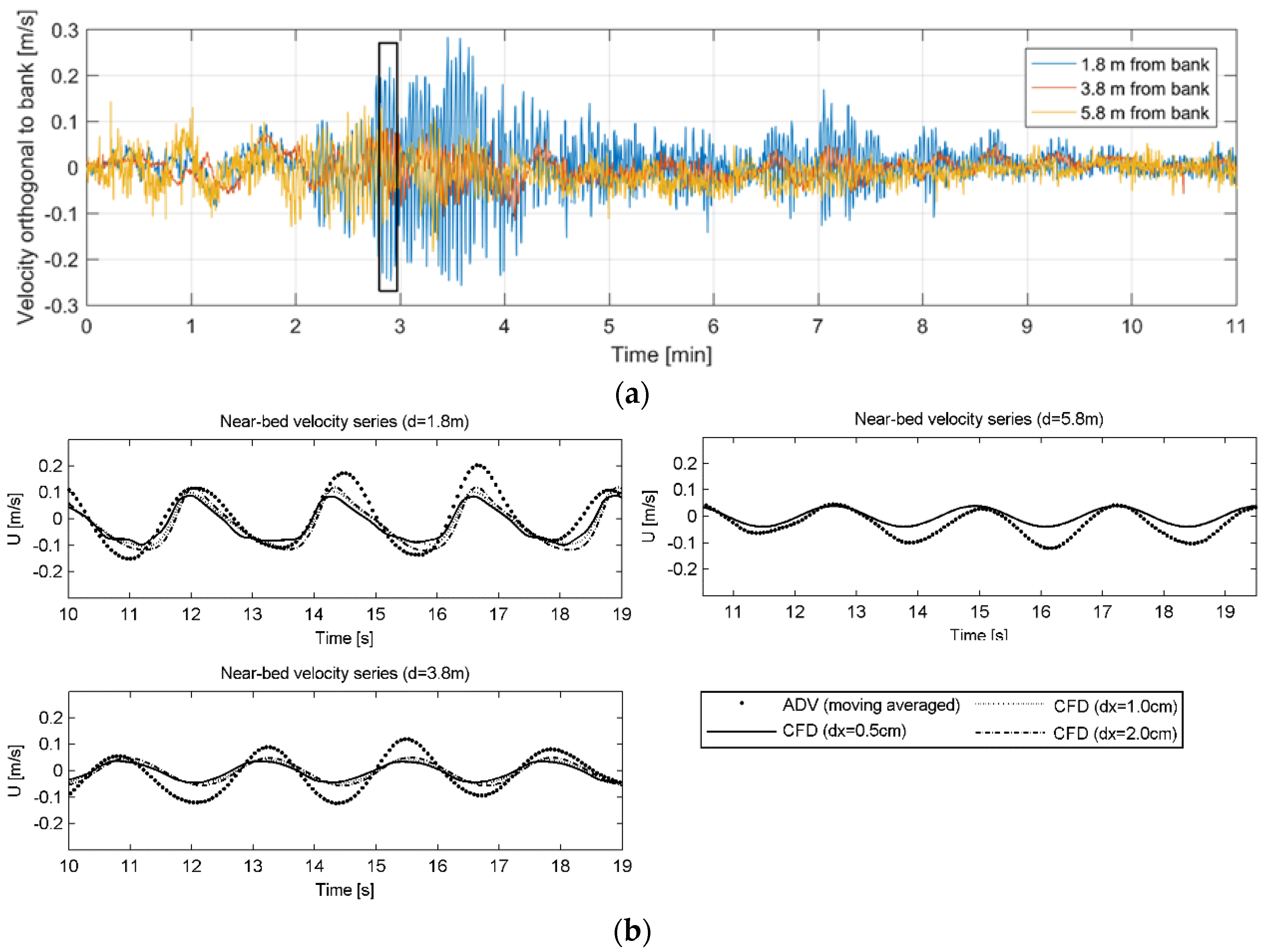
Section 2.4.2. The simulations were performed for the same period where the LSPIV was employed (during the most intense interval of passenger vessel #1 waves). For model validation, we used the measured near-bed velocity time series at the three measurement locations. Specifically, calculated velocity time series were queried in the numerical model at 1.8 m, 3.8 m and 5.8 m distances from the bank line, respectively, right above the bed, exactly at the same locations where the ADV measurements were conducted in the field. The left boundary conditions for incoming waves were properly defined as already shown in
Figure 6. First, a sensitivity analysis was performed to investigate the effect of the grid resolution on the simulation results.
Figure 13 presents the comparison of the
x-wise components of the wave induced near-bed velocities for the three sampling points.
The model seems to underestimate the near-bed velocities, which might be a result of the simplifications made in order to decrease computational times. It is noted that the real flow problem, which is represented by the measured data, having a spatial behavior as shown in
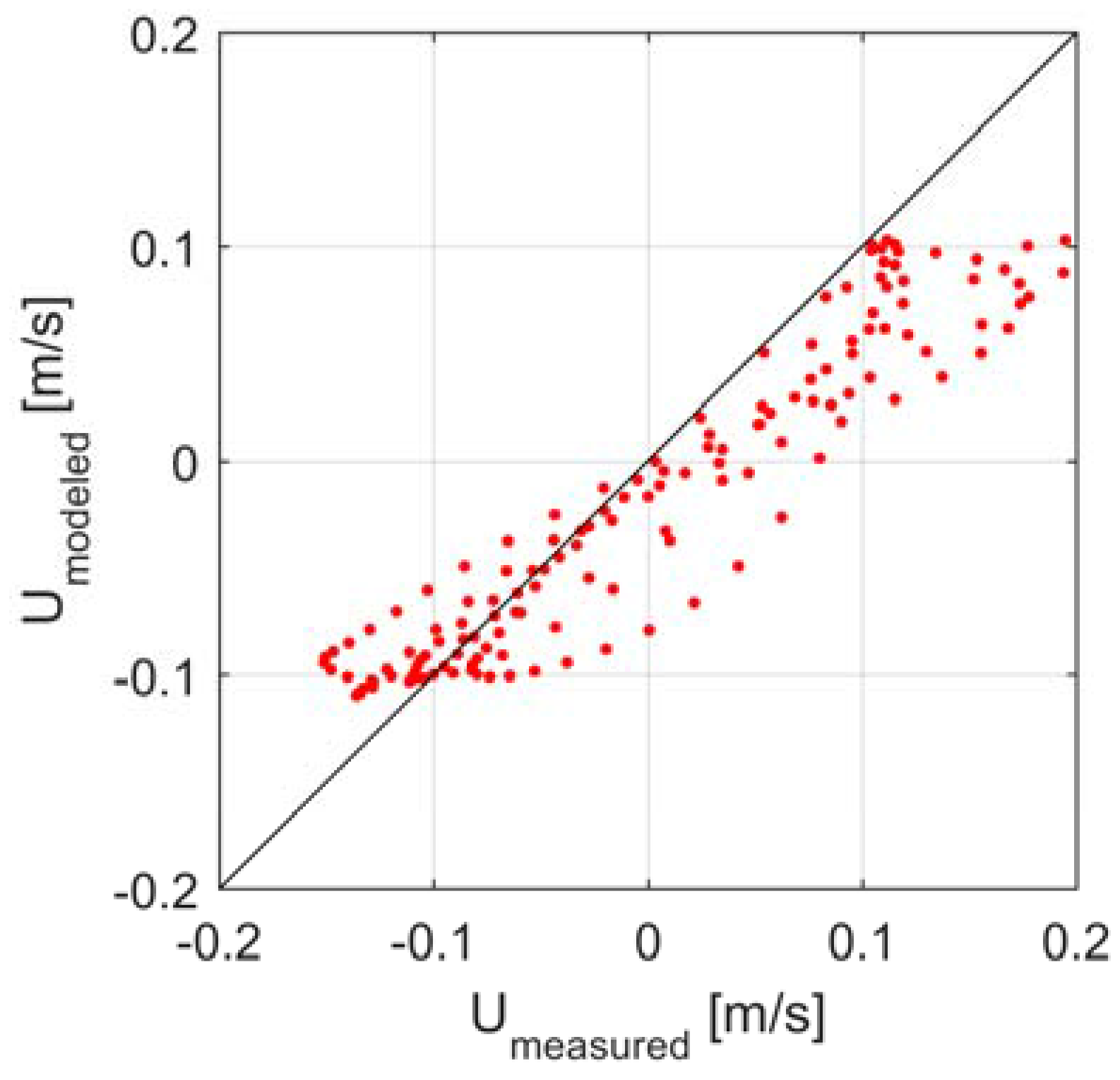
Figure 9, is more complex than the modeled situation; therefore, a perfect match cannot be expected. However, the best match is observed closest to the bank which is the most crucial zone from ecological aspects, since, as already introduced above, the strongest influence of waves is expected here. A scatter plot of the measured and calculated velocities for this point, using the highest grid resolution (d
x = 0.5 cm) is shown in
Figure 14. Indeed, the overall agreement is acceptable, but an underestimation of the velocities by the CFD model can be observed due to the 3D nature of the wave velocities, which is not reproduced by the slice model.
The shallower the water, the more sensitive the solution becomes to the grid resolution. Closest to the inlet section of the numerical model, at a distance of 5.8 m from the bank the three simulated velocity time series are overlapping (
Figure 13b top-right) i.e., at this point the numerical solution is not sensitive to the grid resolution. At a distance of 3.8 m from the bank (
Figure 13b, bottom-left) slight deviations are noted between the simulation results. The amplitude of the velocity time series are very similar, however, a minor phase shift can be noticed.
Figure 13b (top-left) presents the results of the sensitivity analysis for the measurement point closest to the bank (1.8 m). Noticeable differences can be observed in the amplitudes of the velocity series: the velocities decrease with increasing grid resolution. Moreover, with the finer grids, the time series lose their smoothness, and a slight disturbance is observed. This can be explained as the following: when the wave crests reach the bank (in fact, they break before it), the water starts flowing back from the bank in the direction of the river. This is a classic wetting-drying problem, which is increasingly better resolved due to finer grids. The more and smaller cells make the numerical treatment of the phenomenon smoother, and smaller water volume stays on the bank, as the critical water level for the drying criterion becomes smaller with the cell size. This way, a larger volume of water heads back in the direction of the river, with higher momentum, having a stronger effect on the next approaching wave, and consequently on a larger part of the whole domain at the same time.
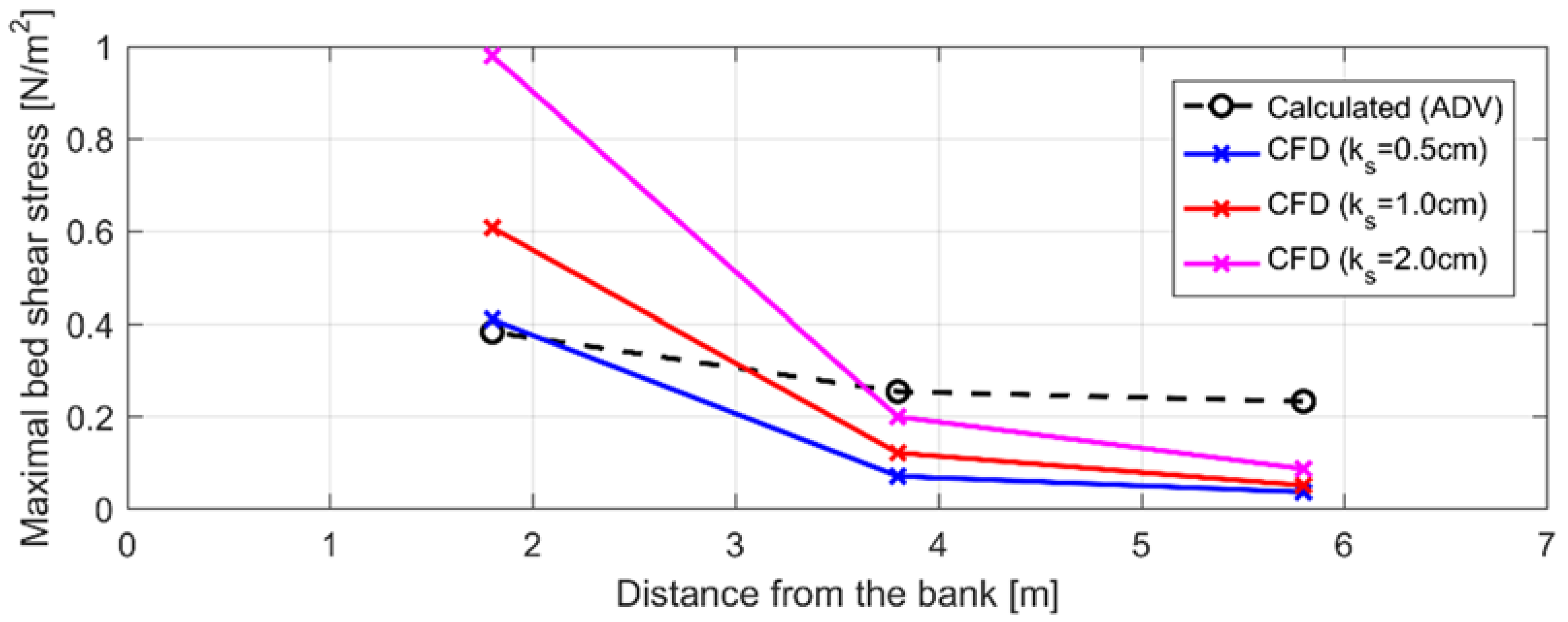
Maximal bottom shear stress was evaluated for the modeled section of the measurements with the Jonsson method and was compared with the numerical results, where the shear stress was determined as [
43]
It is known that there is a strong relationship between the bottom shear stress and the roughness height of the substrate; therefore, a sensitivity analysis was also conducted for this parameter.
Figure 15 presents the comparison of the measured (calculated) and modeled bottom shear stress values.
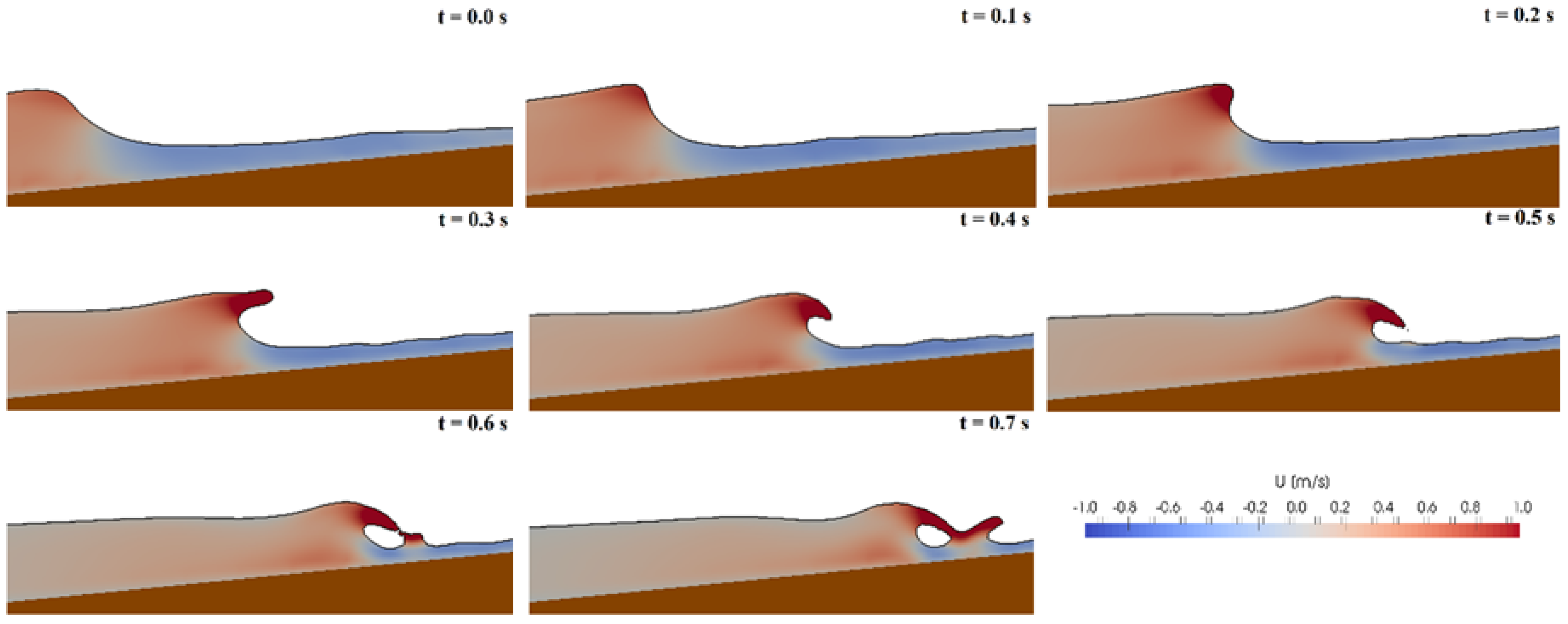
During the field measurements, breaking waves were observed along the riverbank. It is therefore expected that the numerical simulations also reproduce this behavior if the spatial resolution of the model is fine enough. Based on the Irribarren number (Equation (19)), which is a function of wave parameters and geometry, plunging breakers are expected for the present case. Indeed,
Figure 16 presents the breaking (plunging) of a wave for the test case resulted by the CFD model.
The numerical results underline the presence of plunging breakers presented in
Figure 16. The water phase has been colored based on the horizontal velocity component, where red is for the direction towards the bank, blue is towards the river. The results above show that the model is indeed capable to reproduce the phenomenon of breaking waves, moreover, the complex free surface presented in
Figure 16 emphasizes the relevance and the suitability of the level set method applied in the CFD modeling.
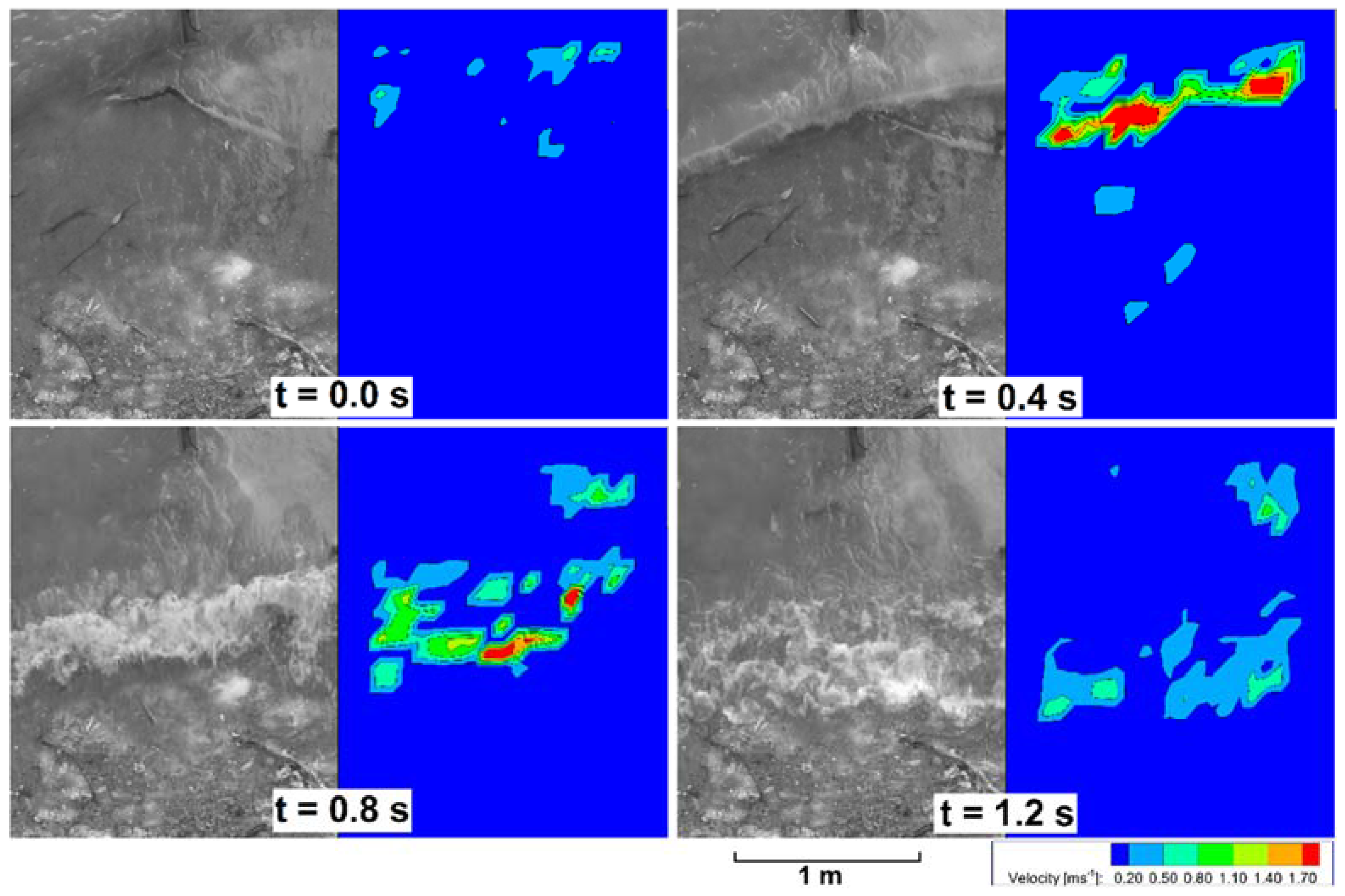
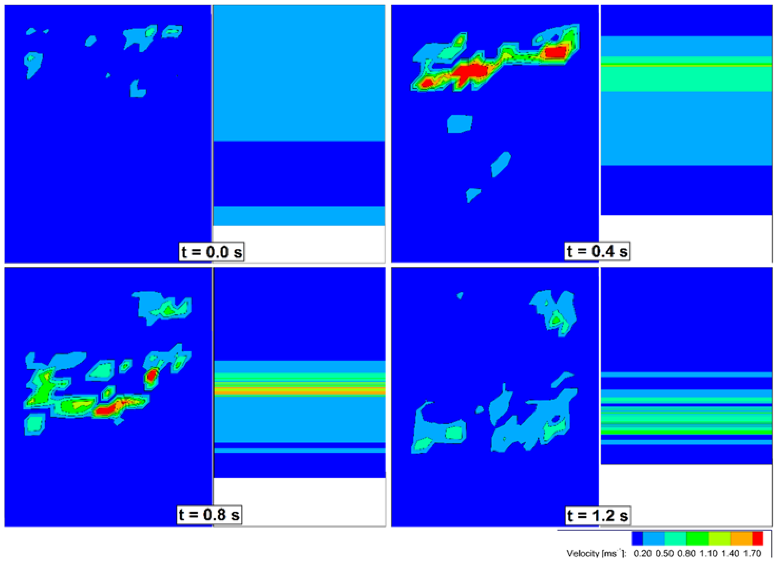
Besides the comparative analysis of simulated near-bed flow velocities using ADV data, a comparison for the velocities of the breaking waves was also performed using the results obtained with LSPIV. Since LSPIV provides two dimensional horizontal velocity distributions at the free surface, simulated velocities had to be provided also from the uppermost modeled layer for the comparison. For a better understanding, the numerical results from the slice model were simply stretched assuming that the waves are unidirectional.
Figure 17 presents the measured (LSPIV) and calculated (CFD) wave propagation velocities at the free surface (the boxes containing the pictures and the LSPIV results are approximately 2.0 m high × 1.5 m wide each).
Despite the fact that two completely different techniques were applied for the wave analysis the main characteristics of the velocity fields match fairly well. Both the LSPIV and the CFD model provide maximal surface velocities for the breaking waves in the range of 1.5–2.0 m·s−1. It has to be noted that the LSPIV method is not able to distinguish the wetted and dried areas, and therefore gives zero velocities for the dried parts as well.
4. Discussion
The potentially negative effects of ship induced waves on riverine habitat have been recognized, however, only very few studies can be found in the literature which attempt to reveal the complex hydrodynamic nature of this phenomenon and link the findings to habitat characteristics. The present study aimed to investigate the waves and currents induced by different ship types in the littoral zone of the Danube, with a major focus on the near-bed region, where the increasing bed shear stress might adversely affect the aquatic ecosystem.
Acoustic measurements, using ADVs, were carried out to reveal the temporally and spatially varying nature of the near-bed velocities, based on which the applicability of different estimation methods for the bed shear stress was also tested. It was shown that the turbulent effects are negligible compared to the larger scale flow features resulted by the waves when estimating bed shear stress. In addition, a significant improvement compared to previous studies was the parallel application of three measurement devices, which pointed out the increasing nature both the velocities and the derived bed shear stress values towards the riverbank.
Besides the acoustic measurements, a novel application of the Large Scale Particle Image Velocimetry (LSPIV) was presented to prove the applicability of this cost-efficient data processing method in the investigation of waves. It was shown that the foam resulted by the breaking waves along the bank is a suitable tracer for the algorithm to track. However, it is clear that the method requires further development and adaptation for the proper treatment of such dynamic and complex phenomena, where the original ideas and assumptions related to the method are not necessarily valid, such as that the surface flow field can be properly characterized with time averaged velocities or the assumption of a constant water level. Moreover, the field deployment and the settings of the camera also requires further development in order to capture larger areas of the water surface and to eliminate the disturbing effect of the stand legs appearing in the frames, where the calculation fails due to its immobility.
The CFD model REEF3D was found to be an adequate and robust computational tool for the simulation of waves. Although the simulations were restricted to a two-dimensional vertical slice, simplifying the actual hydraulic characteristics of ship induced waves, the results show good agreement with measured near-bed velocities and suggest the continuation and extension of the simulations to three-dimensions. As expected, the simulated bed shear stress values were found to be quite sensitive to the bed roughness, however, both the order of magnitude and the tendency towards the riverbank show good agreement with the measurements, however the attenuation is stronger in the model. Considering the hydrodynamic complexity of the simulated phenomenon these first results are more than encouraging and prove the applicability of the chosen numerical tool for such analysis. The results at the same time clearly demonstrate the importance of the information on bed material composition for accurate numerical model parameterization. The CFD model also successfully reproduced the wave breaking, which enhances the stability and relevance of the level set method in multiphase CFD.
Based on the field data a sample application was presented to introduce a likely interconnection of hydrodynamic and ecological parameters, estimating the detachment rate of a macroinvertebrate crab caused by the waves. It was shown that the field data collected with the herein introduced field methodology is suitable to quantify habitat related features. It is noted, that all the methods presented have uncertainties, but it is believed that the combined employment of such field and numerical methods could result in reliable estimation of habitat related parameters such as bed shear stress, which requires very specific instruments for direct measurements [
44].
5. Conclusions and Future Work
The main goal of this study was to present a novel methodology to analyze ship induced waves, combining acoustic, image processing and computational tools, and also to find limits and restrictions of these techniques to support future developments. As to the acoustic measurements, it was found that the main flow features can indeed be quantified, such as highest flow velocity and bed shear stress, but much more information of the complex wave characteristics could be gained with a more sophisticated analysis, which also involves the determination and removal of the background currents, principal component analysis, and spectral analysis. In addition, the extension of the velocity measurements along the vertical, using acoustic profilers such as ADCP could better explain the 3D behavior of wave induced flows. The LSPIV method at the zone of the breaking waves was found to be an effective tool for capturing wave propagation, however, the method introduced here obviously requires further development in order to capture velocities in larger spatial scale and to improve image quality with the usage of some sort of floating tracer or by the elimination of different external disturbances (i.e., tree shadows and stand legs). A major advantage of the LSPIV method is that in contrast with the acoustic velocity measurements, where a single point (volume of 1 cm3) is sampled, it can provide time-dependent horizontal velocity distributions for the free surface. The main goal of the LSPIV based wave measurements is to provide a tool for quantifying the erosion forces caused by breaking waves. As to the numerical simulations, the herein applied solver was found to be an adequate tool for the reproduction of waves and even the breakers with complex free surface. However, as a first attempt on the ship induced wave modeling, certain simplifications were done compared to the real situation, with e.g., simulating a 2D slice model. Clearly, expanding the computational domain to the third dimension, along the bank line, could yield a more detailed description of the flow features. Moreover, the possibility to discretize spatially varying riverbed geometry in 3D could support the design of engineering measures aiming at e.g., the improvement of habitat conditions. Furthermore, as a likely future development of the CFD model, the direct simulation of ship movement and related wave generation would be possible, and so the effect of different ship related parameters (e.g., speed, shape, and load of ships) on the properties of the waves and currents could also be investigated.
The authors believe that the combined field and numerical methods introduced in this study mean a significant improvement compared to existing techniques, however, as described above, there is much more potential in this topic and future developments in several directions are to be done. Nevertheless, it is clear that the hydrodynamic effects of ship induced waves play a unique role in the ecology of the Hungarian Danube, especially in the near-bed regions in the littoral zone, which are important spawning places for fish and habitat for macrobenthos and macrozoobenthos. Due to the multiple uses of the Danube River, which is the second largest river in Europe, it is vital to establish a compromise among the different stakeholders such as ecology and navigation. Moreover, the implementation of the EU Water Framework Directive within the European countries, thus in Hungary as well, enhances the importance of eco-friendly approaches. Improving the investigation tools to reveal the wave phenomena will significantly contribute to this field.


 ,
, 


