Article

Predicting Soil Infiltration and Horizon Thickness for a Large-Scale Water Balance Model in an Arid Environment

1
Faculty of Agriculture, Tottori University, 4-101 Koyama-Minami, Tottori 680-8553, Japan
2
Arid Land Research Center, Tottori University, 1390 Hamasaka, Tottori 680-0001, Japan
3
Department of Materials and Life Science, Seikei University, 3-3-1, Kichijoji-kitamachi, Musashino, Tokyo 180-8633, Japan
4
School of Veterinary and Life Sciences, Murdoch University, 90 South Street, Murdoch 6150 WA, Australia
5
University of Tsukuba, 1-1-1 Tennodai, Tsukuba, Ibaraki 305-8577, Japan
*
Author to whom correspondence should be addressed.
Professor Emeritus.
Water 2016, 8(3), 96; https://doi.org/10.3390/w8030096
Submission received: 16 January 2016 / Revised: 1 March 2016 / Accepted: 3 March 2016 / Published: 10 March 2016
(This article belongs to the Special Issue Water Resources Assessment and Management in Drylands)

Abstract

:
Prediction of soil characteristics over large areas is desirable for environmental modeling. In arid environments, soil characteristics often show strong ecological connectivity with natural vegetation, specifically biomass and/or canopy cover, suggesting that the soil characteristics may be predicted from vegetation data. The objective of this study was to predict soil infiltration characteristics and horizon (soil layer) thickness using vegetation data for a large-scale water balance model in an arid region. Double-ring infiltrometer tests (at 23 sites), horizon thickness measurements (58 sites) and vegetation surveys (35 sites) were conducted in a 30 km × 50 km area in Western Australia during 1999 to 2003. The relationships between soil parameters and vegetation data were evaluated quantitatively by simple linear regression. The parameters for initial-term infiltration had strong and positive correlations with biomass and canopy coverage (R2 = 0.64 − 0.81). The horizon thickness also had strong positive correlations with vegetation properties (R2 = 0.53 − 0.67). These results suggest that the soil infiltration parameters and horizon thickness can be spatially predicted by properties of vegetation using their linear regression based equations and vegetation maps. The background and reasons of the strong ecological connectivity between soil and vegetation in this region were also considered.

1. Introduction

Prediction of soil characteristics over large areas is desirable for environmental modeling, precision agriculture and natural resources management. In arid environments, soil permeability is one of the most important characteristics because it governs infiltration and runoff characteristics of the landscape. Horizon (soil layer) thickness above underground hardpans or basement rocks is also significant because hardpans and basement rocks are impermeable and constrain water movement. These soil characteristics are essential as input parameters or boundary conditions for water balance analysis by rainfall-runoff modeling. Rainfall-runoff models are important to predict the movement of precious water resources in arid landscapes. The accuracy of the input parameters used in such models has a significant effect on model performance [1]. A lack of data for the models is a major limitation for simulation of regional hydrologic processes [2]. However, it is well known that soil characteristics often show high spatial variability. Direct measurements of soil characteristics are time-consuming, labor-intensive and costly to characterize for areas >100 km2.
Stemming from land system surveys of the 1950s to 1970s [3,4,5], two main approaches are widely used to predict the spatial variability of soil characteristics on large scales: geostatistics [6] and environmental correlation [7]. In this paper, we focus on the environmental correlation, specifically using correlations between soil and vegetation properties. An environmental correlation approach evaluates the spatial distribution of soil characteristics by quantifying the relationship between soil and environmental attributes. Terrain attributes derived from digital elevation models (DEM) are the most major predictive factor in this approach [8,9]. Explicit, quantitative, and usually simple empirical models are developed to describe the relationships between georeferenced soil samples and predictive factors (e.g., [10,11]). Multiple linear regression has been most widely used in the modeling processes (e.g., [12,13,14,15]). In addition to the topographical factors, climatic, organic, lithologic and temporal factors can be used as predictors [16].
Land cover is one of the useful indicators of soil properties and class because the natural vegetation and its dynamics should represent some kind of equilibrium relation with soil type [16,17,18]. Recently, vegetation data such as vegetation structure and canopy coverage can be obtained relatively easily even over large areas by remote sensing techniques. These data have been used as predictive factors in combination with terrain attributes and other factors in several studies [19,20,21]. For example, vegetation indices from Landsat Thematic Mapper and Enhanced Thematic Mapper Plus (Landsat TM and ETM+) were used to predict soil classes [22], soil drainage classes [23], soil hydraulic properties [2] and soil profile depth, total phosphorus and total carbon [24]. Zhu [25] used canopy coverage from Landsat TM to predict soil classes. Park and Vlek [26] used a vegetation map to predict soil properties. Vegetation indices from SPOT images were also used to predict soil organic matter [27] and soil organic carbon [28]. In these studies, vegetation data are just one category of the predictive factors, however, successful deployment of this data suggests that the vegetation attributes may play an important role in the environmental correlation approach.
To predict soil infiltration properties and horizon thickness, vegetation factors may be particularly useful because these soil characteristics are highly correlated to vegetation due to the co-evolution of landscapes [29]. A considerable number of studies have been reported on the strong relationship between infiltration parameters and vegetation data (e.g., [30,31,32,33,34,35,36]). Regarding the horizon thickness, Lamotte et al. [37] showed that the depth and distribution of hardpans were associated with differences in vegetation. Pracilio et al. [38] also reported that tree height was limited by the depth to hardpans in southwestern Australia. Therefore, these soil characteristics may be simply predicted from vegetation data only if quantitative and strong correlations can be found between the soil characteristics and vegetation attributes for large areas.
The objective of this study is to investigate the prediction of soil infiltration characteristics and soil horizon thicknesses using vegetation data for areas of the order of hundreds to thousands of km2 in an arid environment. We conducted infiltration tests (at 23 sites), horizon thickness measurements (58 sites) and vegetation surveys (35 sites) in an established research area (30 km × 50 km) in Western Australia. The relationships between obtained soil parameters and vegetation data were evaluated quantitatively by simple linear regression analyses. The infiltration properties and horizon thickness in the whole research area were predicted from regression equations and vegetation maps derived by remote sensing.

2. Area Descriptions and Methods

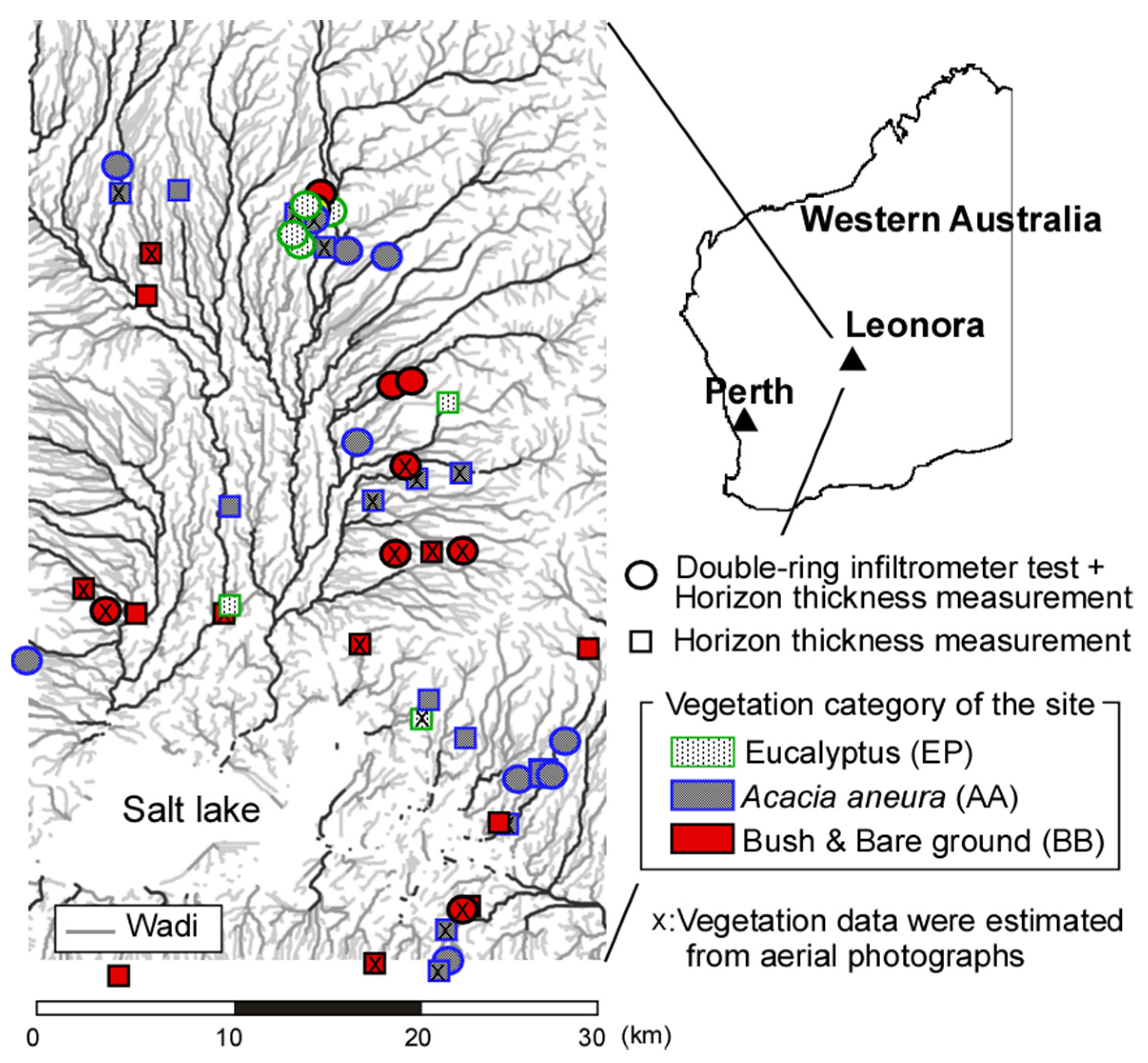
2.1. Research Area and Measurement Sites

The Leonora research area (lat 28°38′13″ S, long 120°59′15″ E) was located about 600 km northeast from Perth, the capital city of Western Australia, covering approximately 1500 km2 (30 km in an east-west direction and 50 km in a north-south direction) (Figure 1). This research area was originally established to assess arid zone afforestation and to estimate the effect of carbon fixation in arid lands [39]. A large-scale water balance model and a tree growth simulator have also been developed to estimate water and carbon flow in the research area [40,41]. Thus, information on soil characteristics for the whole research area was needed for these models and also to establish boundary conditions for the models [42].
The area is arid: average annual rainfall measured in the area (1917–1998) is 211 mm with a standard deviation of 109 mm [43]. Although the topographical gradient is less than 1% for almost the entire research area, there are many wadis (dry riverbeds containing water only during times of heavy rain). When intensive rainfall occurs, the wadis function as drainage paths for runoff to the large and shallow salt lake at the lowest elevation. The surface soil contains abundant quantities of ferric oxide and is colored red due to laterization [44]. The feature of the soil in this area is the presence of the Wiluna hardpan [45], which is extremely hard, impermeable and consists of laminated layers of silica with ferruginous and calcareous cement, and which is often up to 10 m thick [46]. According to a fluorescent X-ray analysis, these hardpans in the research area consist of 45% Al2O3, 39% SiO2 and 12% Fe2O3.
The research area has been used for extensive grazing by one farm family, but all of the forest and woodland in the research area is considered natural forest and woodland [47]. The vegetation of the area is a mixture of Acacia woodland, Acacia shrub land (Acacia aneura with small shrubs, e.g., Eremophilla sp.) and bare ground [47,48]. About half of the research area is bare ground or low open woodland, where canopy coverage is less than 10%, and the other half is woodland and open forest, where canopy coverage varies between 10% and 50% [49]. The dominant species is Acacia aneura; Eucalyptus camaldulensis open forest and woodland are adjacent to some wadis; and salt-tolerant shrubs and bushes are observed around the salt lake. Abe et al. [50] reported that the biomass distribution is related with the slope, position of the wadi and the distance from the wadi.
Measurements on soil infiltration, horizon thickness and vegetation were conducted at a maximum of 58 sites of size 50 m × 50 m. The soil surveys were intensively conducted in November and December in 1999 and 2002. The vegetation surveys were conducted from 1999 to 2003. All sites were classified into three vegetation categories by the dominant species at the sites: Eucalyptus (EP), Acacia aneura (AA), or bush or bare ground (BB) sites. The locations of sites on which measurements were taken were chosen by preliminary ground inspections and interpretation of aerial photographs in order to satisfy the following conditions: (i) the ecological and topographical conditions within each site were homogeneous: and (ii) there was a wide range in the biomass (Figure 1). In addition, the distances of the sites from the nearest wadis were measured by visual interpretations of aerial photographs in order to categorize the sites into “around wadis” (within 100 m of the nearest wadis) and “others”. The reason for the categorization was that the areas around wadis had a characteristic ecosystem. The distribution of wadis was able to be determined also from terrain analysis of a DEM [50].

2.2. Analyzed Data Set

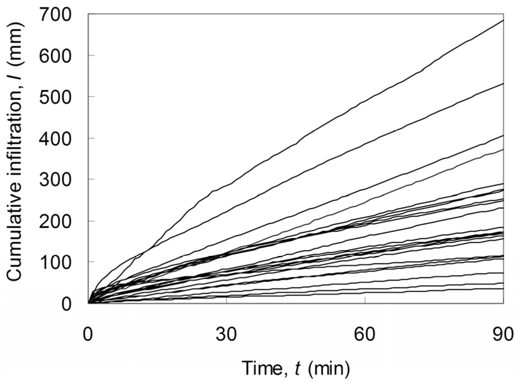
2.2.1. Infiltration Data

Double-ring infiltrometer tests were performed at 23 sites (4 EP, 10 AA and 9 BB sites) (Figure 1). All other variables shown in Section 2.2.2 and Section 2.2.3 were also recorded at these sites. At each site, one point was chosen that gave a satisfactory representation of the surface soil condition of the site. An inner ring, 0.30 m in diameter and 0.30 m deep, was carefully driven 0.10 m into the soil at the chosen point. Each infiltration run continued for 90 min by which time a steady state rate had been attained. Soil profile surveys to measure depth to hardpans were also conducted at all sites at which measurements were made. The horizons were generally dry during the measurement period and the variation of the volumetric water contents was small (0.02–0.08 m3·m−3). The effect of the difference in the soil moisture on infiltration rate was therefore small. At one site with little vegetation, infiltration tests were performed at three locations to evaluate the spatial variability in the soil permeability within the site.
Two commonly used infiltration equations were fitted to the infiltration data collected during tests: the Kostiakov [51] and Philip [52] equations. Cumulative infiltration (I, mm) is expressed by the Kostiakov equation as:
I = ktm,
where t (min) is the time that water has been in contact with the soil, and k and m are constants. The Kostiakov equation is empirical; its parameters do not have clear physical meanings but it is simple and easy to define. Note that if t = 1 in Equation (1), then I = k. This means k is 1 minute of infiltration. In contrast, the Philip equation is based on physical parameters and given by:
I = St1/2 + At,
where S (mm·min−1/2) accounts for the sorption of water at the beginning of the infiltration process and A (mm·min−1) accounts for the long-term (steady-state) infiltration rate. We introduced a parameter It (mm), which is the measured cumulative infiltration for any period of time (t). As above, parameters k, m, S, A and It were obtained as soil infiltration characteristics at each of the sites.
According to visual interpretation of the aerial photographs, six of the 23 sites were within 100 m of the nearest wadis. Analyses excluding these six sites were also performed. A subscript _ew was added to the infiltration parameters when the six sites were excluded in the analyses (e.g., k_ew).

2.2.2. Horizon Thickness Data

Horizon thickness was measured at 58 sites (10 EP, 25 AA and 23 BB sites). The surface horizon above the underground hardpan was dug out by engine augers and the horizon thickness (Th, cm) was determined by measuring the depths of the augered holes. The horizon thicknesses sometimes varied within a short distance thus they were measured at 10–15 locations within each site area, and the average horizon thickness was adopted as the Th data at the site. The maximum measurement range of Th was limited to 115 cm by the length of the drill. Therefore, at 10 sites (seven EP and three AA sites) where the horizon thickness was over 115 cm, Th was tentatively assigned a value of 115 cm. Analyses excluding these 10 sites were also performed.

2.2.3. Vegetation Data

The stand biomass (Bm, kg·m−2) and canopy coverage (Cc, m2·m−2) were measured or estimated at every site. The stand biomass was defined as the sum of the biomass of the individual trees above ground that comprised stand per the unit ground area. The canopy coverage was defined as the ratio of the vertical projection area of the forest and woodland canopy per unit area [47]. Cc was obtained relatively easily from both vegetation surveys and remote sensing analyses. In contrast, Bm was more difficult to estimate than Cc but we considered that it was a more efficacious measure of the amount of vegetation.
At 35 of the 58 sites, vegetation surveys were conducted originally for the remote sensing analyses. Various vegetation parameters were measured for all trees such as tree height, diameter at breast height and canopy silhouette area. Each tree biomass was calculated by the allometric equation for each tree species using a destructive sampling method [53]. From these results, the values of Bm and Cc were calculated for each site. To extrapolate the site based Bm and Cc values to the entire study area, satellite images (Landsat TM and ETM+; 16 scenes from June 1998–December 1999; 30 m resolution) and aerial photographs (on 10–11 November 1999; digitized ortho color photograph consisted of Red, Green and Blue bands, 0.25 m quadrate) were used. As results of analyses for both images, distribution maps of Bm and Cc were made for the entire area. The details of the estimation methods adopted are described by Taniguchi et al. [54] and Suganuma et al. [47,49]. An example of the Bm distribution map developed by satellite image analyses is shown in Figure 2 [54]. At 23 sites at which vegetation surveys were not conducted (Figure 1), Bm and Cc were estimated from the aerial photographs that had higher resolution and accuracy than the satellite images. The Cc values were estimated by visual interpretation of the aerial photographs (e.g., R2 = 0.99 [49]). The Bm values were estimated using high correlation between Bm and Cc for each vegetation type (e.g., R2 = 0.92 [47]).

2.3. Data Analysis and Development of Prediction Equation

Liner regression analysis was used to quantify relationships between the infiltration parameters or horizon thickness and vegetation data. In this paper, soil characteristics were predicted from vegetation data, thus k, m, S, A, It and Th were used as the dependent variables (y) and Bm and Cc were used as the independent variables (x). In addition to regression parameters, some statistical measures were provided to evaluate the model performance: mean (M) and standard deviation (SD) for each observed and predicted variable, mean bias error (MBE) and root mean square error (RMSE) [55].
The dependent variables highly correlated with the vegetation variables were predicted using their linear regression based equations. Prediction equations of time series of infiltration were also developed by substituting the regression equations for each infiltration constant into the original infiltration equations (Equations (1) and (2)). The detailed development is shown in the results section (Section 3.2).

3. Results

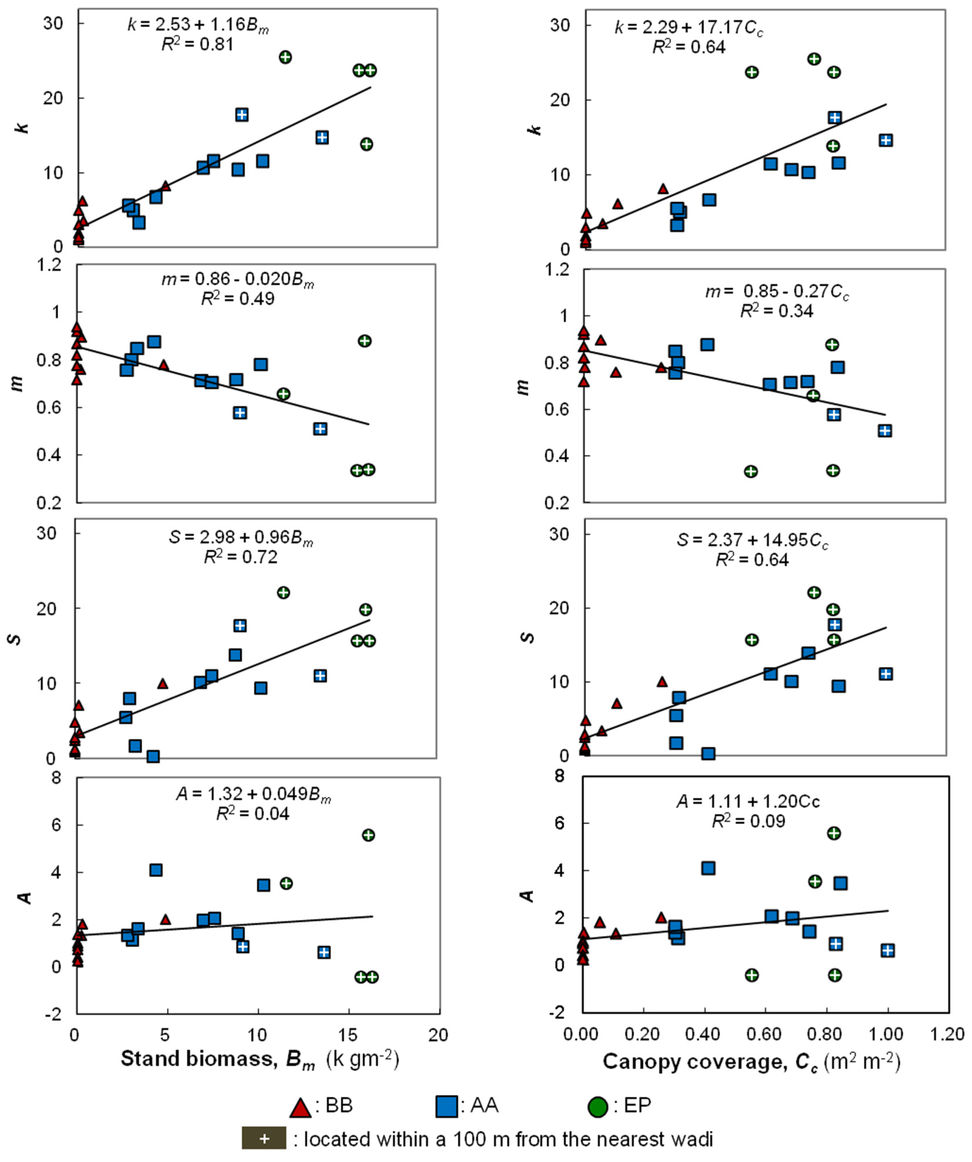
3.1. Relationships between Infiltration Parameters and Vegetation Data

The cumulative infiltrations varied greatly from site to site, suggesting a high spatial variability in the soil permeability in the research area (Figure 3). At a final cumulative infiltration (90 min), the maximum value was 685 mm, minimum 37 mm, mean 226 mm and standard deviation 155 mm. Both Equations (1) and (2) were in close agreement with the measured cumulative infiltration at every site; The coefficients of determination of the fittings were within a range of 0.99 to 1.00, and the RMSE between the measured and fitted cumulative infiltrations were within a range of 0.45 mm to 10.0 mm. At one site where the infiltration tests were performed at three locations, the final cumulative infiltrations (I90) of three tests were 180, 193 and 214 mm and the standard deviation was 17 mm, suggesting the spatial variability in the soil permeability was small within the site.
Table 1 shows the output of the resulting linear regression analysis relating vegetation data to infiltration parameters and statistical measures. Several infiltration parameters correlated highly with vegetation data. The constants k in the Kostiakov equation and S in the Philip equation showed particularly high and positive correlations with Bm and Cc (Figure 4). Both k and S are measures of the infiltrability at the beginning of the infiltration process and results indicate that surface soil permeability was strongly correlated with the vegetation. With an increase in the t value of It, the correlation coefficients between It and Bm or Cc decreased (Table 1). Thus, the rate of infiltration into shallower soil has a stronger correlation with vegetation. No significant correlation was obtained between the constant A of Philip’s equation and Bm or Cc. This result suggests that permeability of horizons low in the profile is not correlated with the vegetation because the constant A accounts for the long-term infiltration rate.
When the six sites within 100 m of the nearest wadis were excluded from the regression analyses, the R2 values between I60_ew or A_ew and the vegetation data substantially increased compared with those of I60 or A (Table 1). The initial infiltrability, k_ew and S_ew, also showed a strong correlation with vegetation data, suggesting that the soil permeability from the surface to depth is strongly correlated with the vegetation except close to wadis.

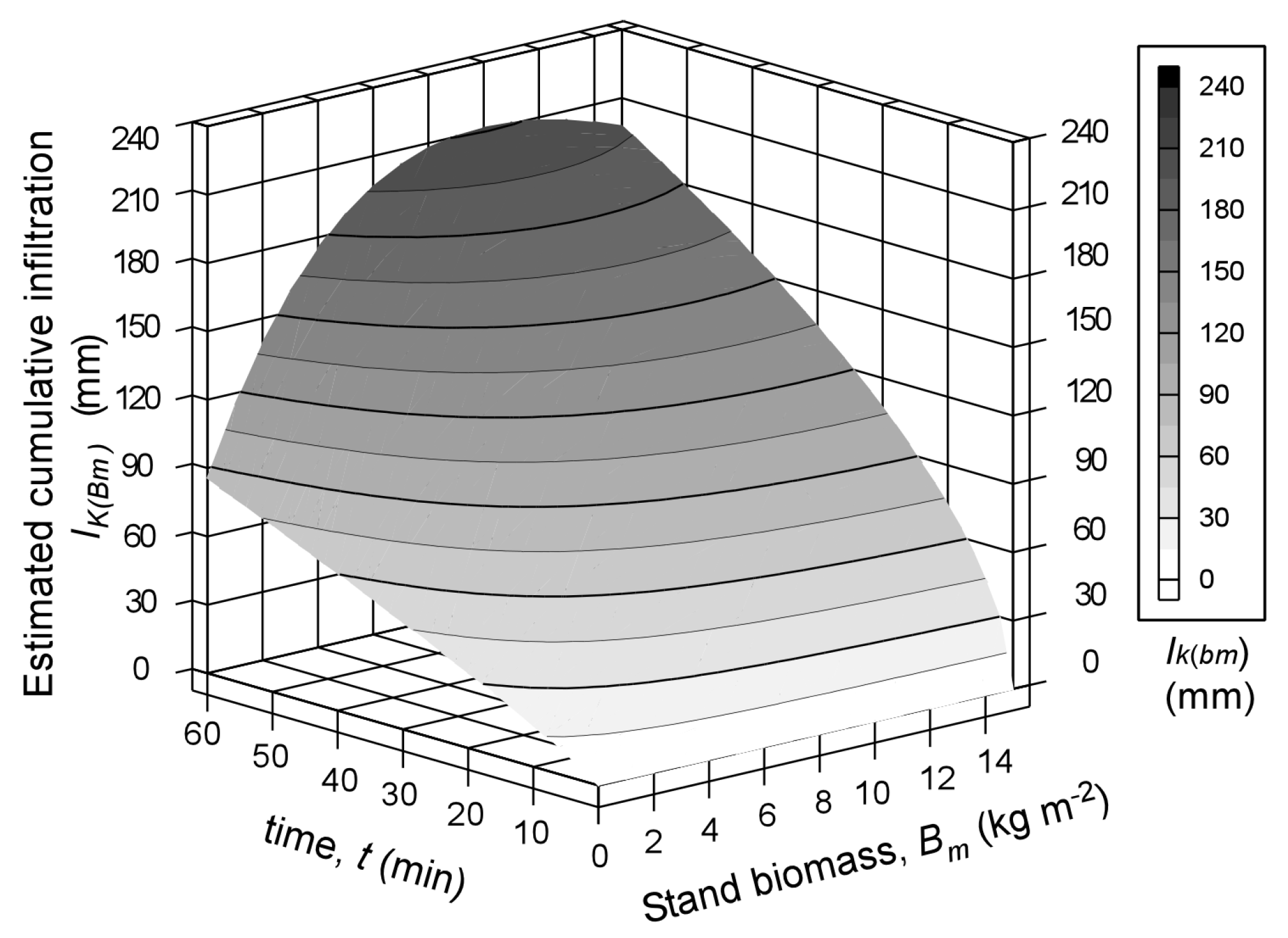
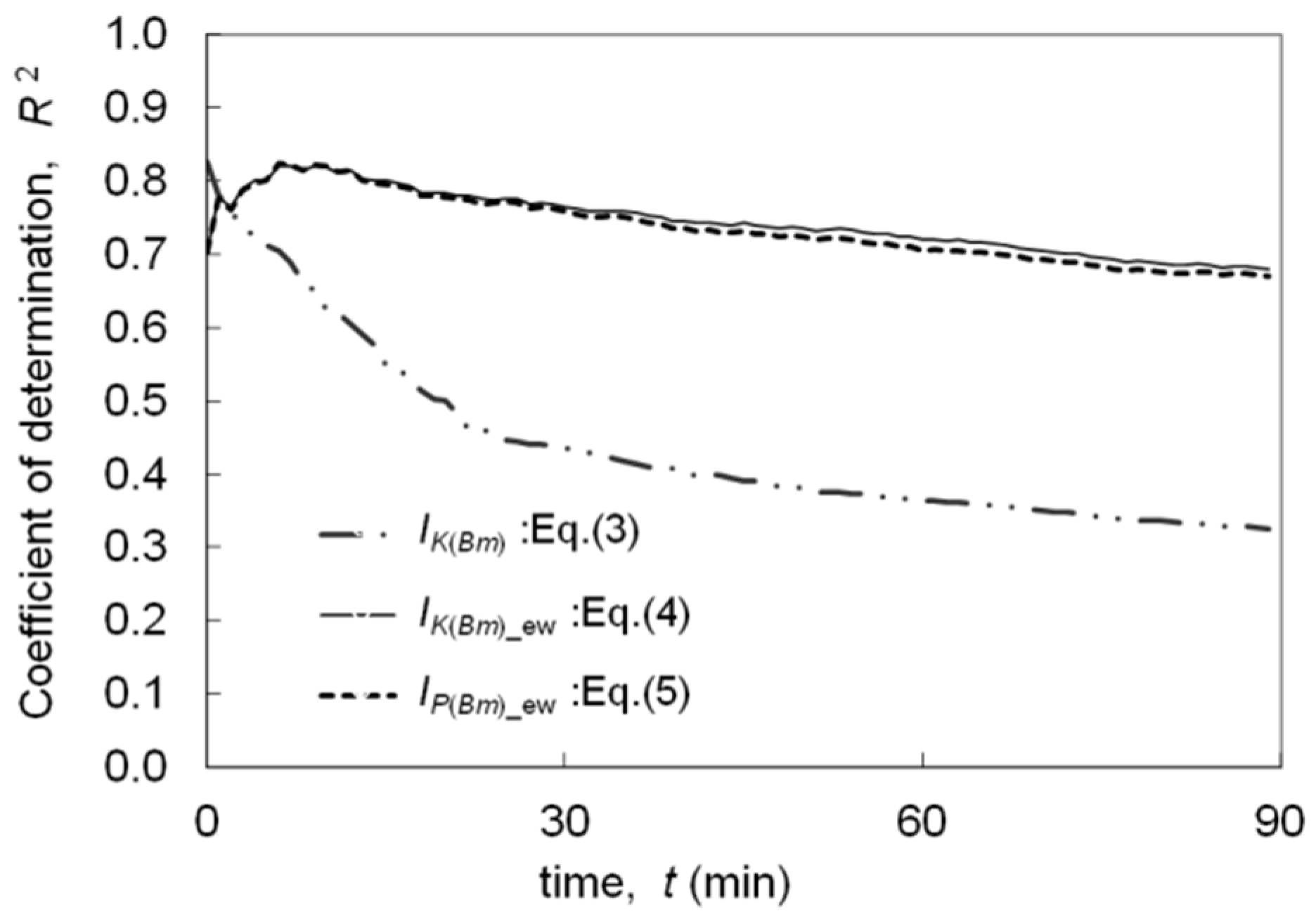
3.2. Prediction of Infiltration Parameters from Vegetation Data

The initial infiltrability (k, S and I5) can be predicted with high accuracy from Bm and Cc over the whole area using the linear regression coefficients shown in Table 1. For example, S (sorptivity: mm·min−1/2) can be expressed as a function of Bm using S(Bm) = 2.98 + 0.96Bm from Figure 4, where S(Bm) is the estimated sorptivity from Bm. Using this equation, Figure 2 is regarded as the distribution map of S for the whole research area. The long-term infiltrability (I60 and A), which was poorly correlated, was not predicted for the whole area, however, it can be predicted as well as the initial infiltrability if the area of within 100 m wadis is eliminated. I60 is an important long-term infiltrability parameter because it is used to model hourly runoff generation when hourly rainfall data are available. I60_ew showed a strong correlation with Bm and Cc. Therefore, the prediction of hourly runoff becomes possible by the concurrent use of the hourly rainfall data, the regression equation for I60_ew, and distribution maps of wadis and Bm or Cc.
An example of the development of the prediction equation of time series infiltration, using the relationship between k, m and Bm is given below. Both constants k and m of the Kostiakov equation are closely correlated with Bm. The regression equations between k and Bm, and m and Bm from Table 1 are k = 2.53 + 1.16Bm and m = 0.86 − 0.020Bm. Substituting these into Equation (1) gives the estimated cumulative infiltration, IK(Bm) (mm), as:
IK(Bm) = (2.53 + 1.16Bm)t−0.020Bm+0.86.
Simultaneous use of Equation (3) and the Bm distribution map (Figure 2) enables the prediction of cumulative infiltration at any elapsed time and at any place in the area. The value of IK(Bm) increases with increases in t and Bm (Figure 5). However, at high values of t and Bm, IK(Bm) decreases with an increase in Bm. The decrease in IK(Bm) with the increase in Bm is incongruous with the observed positive correlation between infiltrability and vegetation.
A similar procedure was used for the other infiltration parameters. The relationships between k_ew and m_ew for Equation (1), and S_ew and A_ew for Equation (2) are shown below. The prediction equations are presented as, respectively:
IK(Bm)_ew = (2.69 + 0.95Bm)t−0.011Bm+0.84,
IP(Bm)_ew = (2.69 + 0.91Bm)t1/2 + (1.05 + 0.17Bm)t,
where IK(Bm)_ew and IP(Bm)_ew are the estimated cumulative infiltrations in mm. The subscript K and P denote that the bases of the equations are Kostiakov and Philip equations, respectively. These equations can be applied to the study area excluding the wadi surrounds.
The prediction accuracy of Equations (3)–(5) was evaluated by the coefficient of determination (R2) between the estimated cumulative infiltration and It (measured cumulative infiltration) for all sites. Figure 6 presents the variations in the R2 values with time. The R2 value between IK(Bm) and It was initially high (R2 > 0.6, t < 10 min), but decreased rapidly with time because of: (i) the low correlation between long-term infiltrability and vegetation; and (ii) the decrease in IK(Bm) with the increase in Bm in the high ranges of t and Bm (Figure 5), as previously mentioned. We propose that Equation (3) should be used only for the prediction of initial-term infiltrations, such as for the prediction of infiltrations and runoff generations for brief rainfall events (t < 20 min). In contrast, the R2 value between IK(Bm)_ew or IP(Bm)_ew and It was more than 0.7 for all time periods, suggesting that even long-term infiltration can be predicted by Equations (4) or (5) with an acceptable degree of accuracy in the area outside the wadi surrounds. There was no significant difference between Equations (4) and (5) in prediction accuracy. The RMSE between the measured cumulative infiltration and IK(Bm), IK(Bm)_ew and IP(Bm)_ew at 60 min were 83.5, 35.6 and 36.0 mm, respectively. These values were slightly smaller than the RMSE values of Bm-I60 and Bm-I60_ew (Table 1), suggesting the developed time series equations predicted the cumulative infiltration more accurately than the original regression equations.

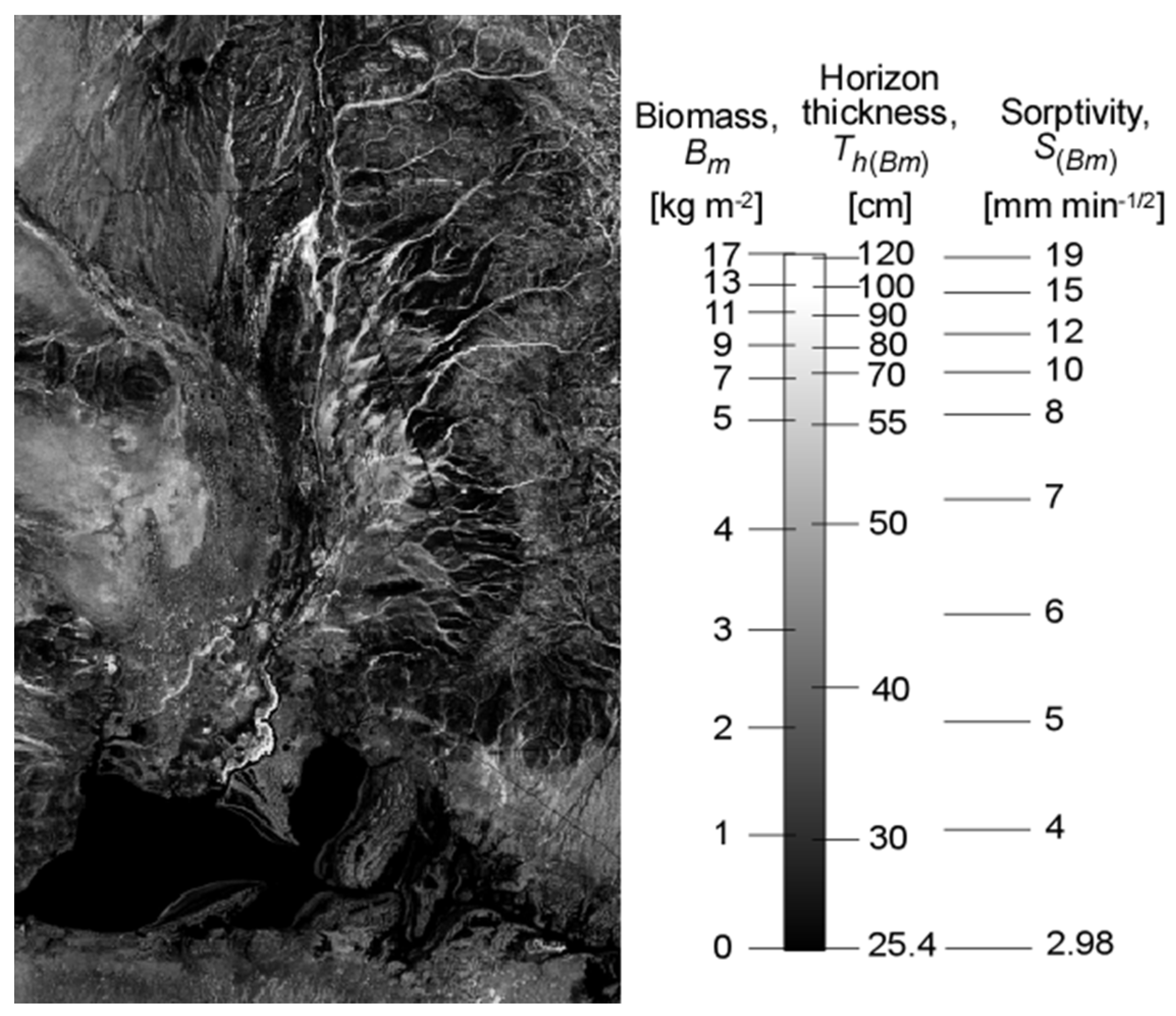
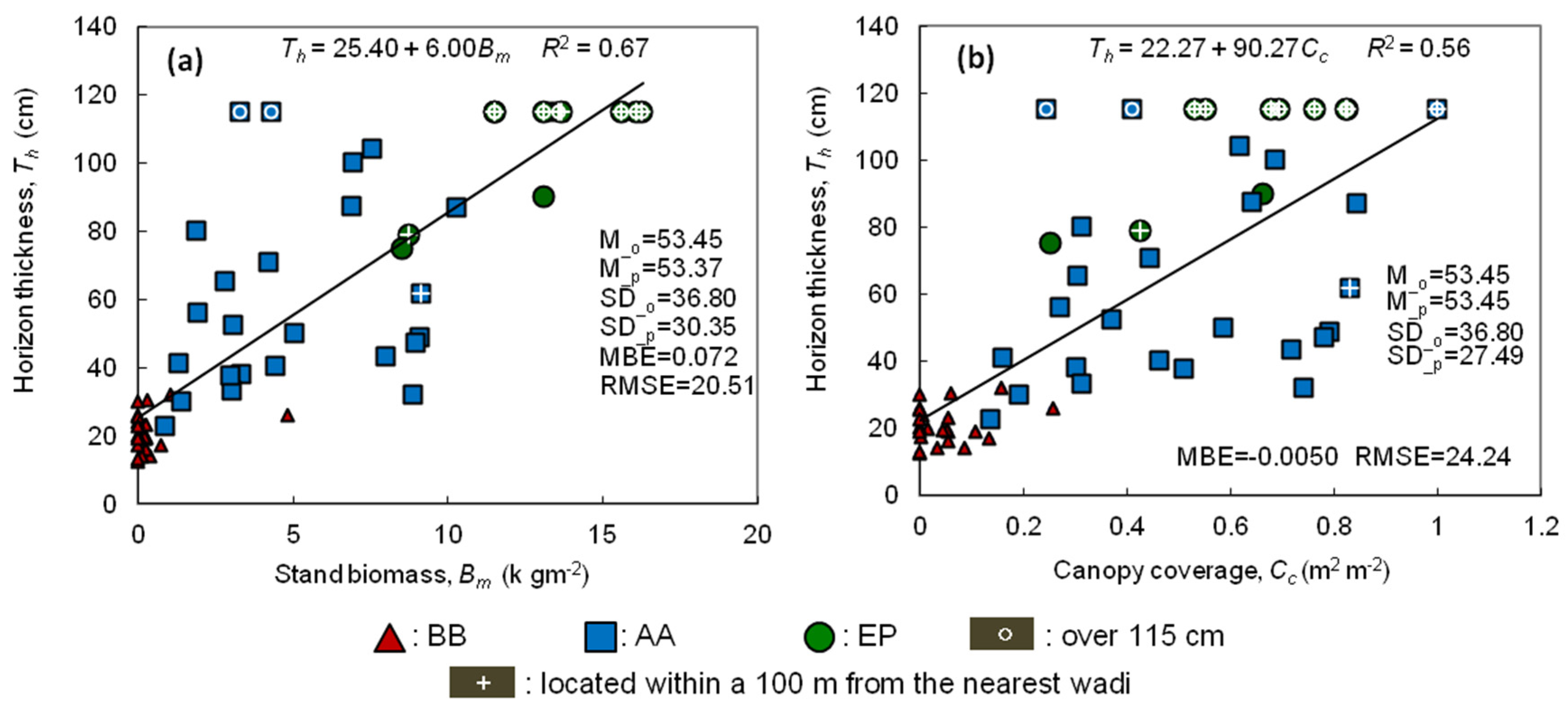
3.3. Prediction of Horizon Thickness from Vegetation Data

The horizon thickness had strong positive correlations with Bm (R2 = 0.67; n = 58; p < 0.001) and Cc (R2 = 0. 56; n = 58; p < 0.001) (Figure 7). Th can be expressed as a function of Bm using Th(Bm) = 25.40 + 6.00Bm from Figure 7a, where Th(Bm) is the estimated horizon thickness from Bm in cm. Using this equation, Figure 2 is regarded as the distribution map of Th for the whole research area. When 10 sites, the horizon thicknesses of which were greater than 115 cm were excluded in regression analyses, Th showed strong correlation with Bm (R2 = 0.58; n = 48; p < 0.001) and Cc (R2 = 0.53; n = 48; p < 0.001), meaning the excluding these sites does not affect the correlation relationship. Eight of these 10 sites and another two sites were located within 100 m of the nearest wadi. If the total of 12 irregular sites, Th > 115 cm or around wadis, were excluded in regression analyses, Th still showed strong correlation with Bm (R2 = 0.55; n = 46; p < 0.001) and Cc (R2 = 0.53; n = 46; p < 0.001).

4. Discussion

The six sites within 100 m of the nearest wadis had relatively high Bm and Cc values, and showed high initial infiltration rates (Figure 4). From the result of soil profile surveys, horizons with low permeability were observed at three of these six sites. The depths of these horizons were about 20–50 cm from the soil surface. Although these horizons were not hardpans, they were extremely compacted and hard; the values for the long-term infiltration parameters were strongly affected by them. It seemed that these horizons of low permeability served as transient river beds around wadis during large runoff events. In contrast, there were no horizons of low permeability in the other three sites within 100 m of wadis and the soil permeability was high even at depth. These results indicate that the spatial variability of permeability was particularly high in lower horizons around wadis.
The constant m in the Kostiakov equation had a negative and strong correlation with Bm and Cc (Figure 4). This constant does not have clear physical meaning, but when the m value is small, the infiltration rate rapidly decreases with time (Equation (1)). Thus, m values were particularly small at the three sites around wadis where there are horizons of low permeability. These m values enhanced the negative slope of the regression line (b) between m and Bm or Cc (Table 1 and Figure 4). Therefore, the slope values of m_ew for both Bm and Cc were smaller than the slope values of m for Bm and Cc. The prediction equation of time-series infiltration was also affected by the steep negative gradient due to the small m values; this was the reason why the predicted IK(Bm) by Equation (3) decreased with an increase in Bm at high values of t and Bm (Figure 5).
BB (bush or bare ground) sites were concentrated in the lower range of k and S, and the lower range of Bm and Cc (Figure 4). In contrast, EP (Eucalyptus) sites concentrated in the upper range of k and S, and Bm and Cc, respectively. AA (Acacia aneura) sites were distributed along regression lines, which means the stand biomass and canopy coverage of Acacia aneura spatially varied and correlated with the surface soil permeability.
It appeared that the main reason for the strong correlation between horizon thickness and vegetation was the restriction of the rooting depth for plants in the vicinity of hardpans [38,56]. Furthermore, vegetation may also affect the horizon thickness as a natural selection process and for its advantage [57,58,59]. For example, rich vegetation supplies surface soils through litter falls and micro-organisms, in contrast, poor vegetation cover often causes runoff and erosion which reduces the horizon thickness. BB sites were concentrated in the lower ranges of Th and Bm or Cc, whereas EP sites were concentrated in higher ranges (Figure 7). These tendencies were similar to the distributions of BB and EP shown in the relationships between initial infiltrability and vegetation data (Figure 4). AA sites were dispersed widely in thin to deep soil areas; Acacia aneura may be able to grow regardless of the limitation of depth to the hardpan. This would be one of the reasons why Acacia aneura was the dominant species in this area where hardpans distribute in shallow underground.
It seemed that the strong correlation between soil infiltration, horizon thickness and vegetation was caused by their ecological connectivity through water movement. Such associations may be particularly pronounced in arid lands because water is the main driving force of vegetation distribution and hence ecosystems in arid environments (e.g., [60,61,62]). The regression equations presented in this paper are region-specific. We contend that the same concept of prediction of these soil characteristics would be applicable for other arid lands that have similar ecosystems.
In most cases, above ground stand biomass showed slightly higher correlations with soil characteristics than canopy coverage (Table 1). We propose that this was because the stand biomass obtained in this study included the allometric equation for each tree species in the calculation, and hence it was a more robust measure of the current condition and amount of vegetation than canopy coverage. However, canopy coverage can be obtained more easily than biomass. The choice of either stand biomass or canopy coverage as the predictor will depend on the required accuracy and the resources required to collect the field data.
Strong statistical relationships are proven between vegetation indices calculated from satellite imagery such as NDVI (Normalized Difference Vegetation Index) or SAVI (Soil Adjusted Vegetation Index) and biomass or canopy coverage. Vegetation indices can be obtained more easily for even larger areas than our current study site; they may be able to be effective soil characteristic predictors. Further studies are required to explore other predictors based on remote sensing. Improvement of field measurements is another task. To determine depths to deep hardpans, electric resistivity surveys may be useful [37]. We used the double-ring infiltrometer for the convenience of use and transportation; however, infiltrability is often overestimated under ponding conditions compared with dripping conditions (e.g., [63,64]). Quantification of spatial variability of infiltrability within sites may also be important, specifically at high vegetation sites. Conducting multiple infiltration tests within a site using rainfall simulators will contribute to increase in accuracy of runoff prediction.

5. Conclusions

Soil infiltration characteristics and horizon thickness were predicted using vegetation data for a 1500 km2 site in an arid environment. The parameters for the initial-term infiltration and horizon thickness had strong and positive correlations with the biomass and canopy coverage over the entire area studied. The parameters for the long-term infiltration also had strong, positive correlations with vegetation when the data obtained around wadis was excluded. We conclude that the infiltration parameters and horizon thickness above hardpans can be predicted by use of the linear regression equations with vegetation data. The prediction equations of time series infiltration were developed by substituting the regression equations for each infiltration parameter into the original infiltration equations. Concurrent use of these equations and the distribution map of vegetation (and wadis) enabled the prediction of the cumulative infiltration at any time for place in the research area. We contend that the same concept of prediction of soil characteristics would be applicable for other arid lands that have similar ecosystems.

Acknowledgments

This work was conducted under the supports of the Global Environment Research Fund of The Ministry of Environment (GHG-SSCP Project), CREST of JST (Japan Science and Technology Agency) and International Platform for Dryland Research and Education, Tottori University. We thank Masahiko Taniguchi for providing data and helpful discussions.

Author Contributions

Tadaomi Saito, Hiroshi Yasuda, Yukuo Abe and Toshinori Kojima conceived and designed the experiments; Tadaomi Saito and Hideki Suganuma performed the experiments; Tadaomi Saito and Koji Inosako analyzed the data; Tadaomi Saito wrote the paper.

Conflicts of Interest

The authors declare no conflict of interest.

References

  1. Guo, W.; Wang, C.; Zeng, X.; Ma, T.; Yang, H. Subgrid Parameterization of the Soil Moisture Storage Capacity for a Distributed Rainfall-Runoff Model. Water 2015, 7, 2691–2706. [Google Scholar] [CrossRef]
  2. Sanjay, K.S.; Mohanty, B.P.; Zhu, J. Including topography and vegetation attributes for developing pedotransfer functions. Soil Sci. Soc. Am. J. 2006, 70, 1430–1440. [Google Scholar]
  3. Barshad, I. Factors affecting clay formation. In Proceedings of the 6th National Conference on Clays and Clay Mineralogy, Berkeley, CA, USA, 19–23 August 1957; pp. 110–132.
  4. Nye, P.H.; Greenland, D.J. The Soil under Shifting Cultivation; Commonwealth Bureau of Soils: Harpenden, UK, 1960. [Google Scholar]
  5. Giltrap, D.J. Mathematical Techniques for Soil Survey Design. Ph.D. Thesis, University of Oxford, Oxford, UK, 1977. [Google Scholar]
  6. Chilès, J.P.; Delfiner, P. Geostatistics: Modeling Spatial Uncertainty; Wiley: New York, NY, USA, 1999. [Google Scholar]
  7. McKenzie, N.J.; Austin, M.P. A quantitative Australian approach to medium and small scale surveys based on soil stratigraphy and environmental correlation. Geoderma 1993, 57, 329–355. [Google Scholar] [CrossRef]
  8. Gallant, J.C.; Wilson, J.P. Primary Topographic Attributes. In Terrain Analysis; Wilson, J.P., Gallant, J.C., Eds.; John Wiley & Sons, Inc.: New York, NY, USA, 2000; pp. 51–85. [Google Scholar]
  9. Maynard, J.J.; Johnson, M.G. Scale-dependency of LiDAR derived terrain attributes in quantitative soil-landscape modeling: Effects of grid resolution vs. neighborhood extent. Geoderma 2014, 230, 29–40. [Google Scholar] [CrossRef]
  10. McSweeney, K.; Gessler, P.E.; Slater, B.; Hammer, R.D.; Bell, J.C.; Petersen, G.W. Towards a new framework for modeling the soil-landscape continuum. In Factors of Soil Formation: A Fiftieth Anniversary Retrospective; Amundson, R.G., Tandarich, J., Harden, J., Singer, M., Luxmoore, R.J., Bartels, J.M., Eds.; Soil Science Society of America, Inc.: Madison, WI, USA, 1994; pp. 127–145. [Google Scholar]
  11. Thompson, J.A.; Pena-Yewtukhiw, E.M.; Grove, J.H. Soil-landscape modeling across a physiographic region: Topographic patterns and model transportability. Geoderma 2006, 133, 57–70. [Google Scholar] [CrossRef]
  12. Moore, I.D.; Gessler, P.E.; Nielsen, G.A.; Peterson, G.A. Soil attribute prediction using terrain analysis. Soil Sci. Soc. Am. J. 1993, 57, 443–452. [Google Scholar] [CrossRef]
  13. Gessler, P.E.; Moore, I.D.; McKenzie, N.J.; Ryan, P.J. Soil–landscape modeling and the spatial prediction of soil attributes. Int. J. Geogr. Inf. Syst. 1995, 9, 421–432. [Google Scholar] [CrossRef]
  14. Chaplot, V.; Walter, C.; Curmi, P. Improving soil hydromorphy prediction according to DEM resolution and available pedological data. Geoderma 2000, 97, 405–422. [Google Scholar] [CrossRef]
  15. Park, S.J.; McSweeney, K.; Lowery, B. Identification of the spatial distribution of soils using a process-based terrain characterization. Geoderma 2001, 103, 249–272. [Google Scholar] [CrossRef]
  16. McBratney, A.; Mendonça, S.M.; Minasny, B. On digital soil mapping. Geoderma 2003, 117, 3–52. [Google Scholar] [CrossRef]
  17. Donohue, R.J.; Roderick, M.L.; McVicar, T.R. On the importance of including vegetation dynamics in Budyko's hydrological model. Hydrol. Earth Syst. Sci. 2007, 11, 983–995. [Google Scholar] [CrossRef]
  18. Gasch, C.K.; Huzurbazar, S.V.; Stahl, P.D. Small-scale spatial heterogeneity of soil properties in undisturbed and reclaimed sagebrush steppe. Soil Till Res. 2015, 153, 42–47. [Google Scholar] [CrossRef]
  19. Feng, Q.; Zhao, W.; Qiu, Y.; Zhao, M.; Zhong, L. Spatial Heterogeneity of Soil Moisture and the Scale Variability of Its Influencing Factors: A Case Study in the Loess Plateau of China. Water 2013, 5, 1226–1242. [Google Scholar] [CrossRef]
  20. De Carvalho, W.; Chagas, C.D.; Lagacherie, P.; Calderano, B.; Bhering, S.B. Evaluation of statistical and geostatistical models of digital soil properties mapping in tropical mountain regions. Rev. Bras. Cienc. Solo 2014, 38, 706–717. [Google Scholar] [CrossRef]
  21. Fu, T.; Chen, H.; Zhang, W.; Nie, Y.; Gao, P.; Wang, K. Spatial variability of surface soil saturated hydraulic conductivity in a small karst catchment of southwest China. Environ. Earth Sci. 2015, 74, 6847–6858. [Google Scholar] [CrossRef]
  22. Grinand, C.; Arrouays, D.; Laroche, B.; Martin, M.P. Extrapolating regional soil landscapes from an existing soil map: Sampling intensity, validation procedures, and integration of spatial context. Geoderma 2008, 143, 180–190. [Google Scholar] [CrossRef]
  23. Campling, P.; Gobin, A.; Feyen, J. Logistic modeling to spatially predict the probability of soil drainage classes. Soil Sci. Soc. Am. J. 2002, 66, 1390–1401. [Google Scholar] [CrossRef]
  24. McKenzie, N.J.; Ryan, P.J. Spatial prediction of soil properties using environmental correlation. Geoderma 1999, 89, 67–94. [Google Scholar] [CrossRef]
  25. Zhu, A.X. Mapping soil landscape as spatial continua: The neural network approach. Water Resour. Res. 2000, 36, 663–677. [Google Scholar] [CrossRef]
  26. Park, S.J.; Vlek, L.G. Prediction of three-dimensional soil spatial variability: A comparison of three environmental correlation techniques. Geoderma 2002, 109, 117–140. [Google Scholar] [CrossRef]
  27. Liu, S.; An, N.; Yang, J.; Dong, S.; Wang, C.; Yin, Y. Prediction of soil organic matter variability associated with different land use types in mountainous landscape in southwestern Yunnan province, China. Catena 2015, 133, 137–144. [Google Scholar] [CrossRef]
  28. Oueslati, I.; Allamano, P.; Bonifacio, E.; Claps, P. Vegetation and Topographic Control on Spatial Variability of Soil Organic Carbon. Pedosphere 2013, 23, 48–58. [Google Scholar] [CrossRef]
  29. Berry, S.L.; Farquhar, G.D.; Roderick, M.L. Co-evolution of climate, soil and vegetation. In Encyclopedia of Hydrological Sciences; Anderson, M., Ed.; John Wiley: Indianapolis, IN, USA, 2005; Volume 1. [Google Scholar]
  30. Berndtsson, R.; Larson, M. Spatial variability of infiltration in a semi-arid environment. J. Hydrol. 1987, 90, 117–133. [Google Scholar] [CrossRef]
  31. Bruce, R.R.; Langdale, G.W.; West, L.T.; Miller, W.P. Soil surface modification by biomass inputs affecting rainfall infiltration. Soil Sci. Soc. Am. J. 1992, 56, 1614–1619. [Google Scholar] [CrossRef]
  32. Stroosnijder, L. Modelling the effect of grazing on infiltration, runoff and primary production in the Sahel. Ecol. Model. 1996, 92, 79–88. [Google Scholar] [CrossRef]
  33. Weltz, L.; Frasier, G.; Weltz, M. Hydrologic responses of shortgrass prairie ecosystems. J. Range Manag. 2000, 53, 403–409. [Google Scholar] [CrossRef]
  34. Wainwright, J.; Parsons, A.J.; Schlesinger, W.H.; Abrahams, A.D. Hydrology-vegetation interactions in areas of discontinuous flow on a semi-arid bajada, Southern New Mexico. J. Arid Environ. 2002, 51, 319–338. [Google Scholar] [CrossRef]
  35. Rietkerk, M.; Ouedraogo, T.; Kumar, L.; Sanou, S.; Van Langevelde, F.; Kiema, A.; Van de Koppel, J.; Van Andel, J.; Hearne, J.; Skidmore, A.K.; De Ridder, N.; Stroosnijder, L.; Prins, H.H.T. Fine-scale spatial distribution of plants and resources on a sandy soil in the Sahel. Plant Soil 2002, 239, 69–77. [Google Scholar] [CrossRef]
  36. Kelishadi, H.; Mosaddeghi, M.R.; Hajabbasi, M.A.; Ayoubi, S. Nearsaturated soil hydraulic properties as influenced by land use management systems in Koohrang region of central Zagros, Iran. Geoderma 2014, 213, 426–434. [Google Scholar] [CrossRef]
  37. Lamotte, M.; Bruand, A.; Dabas, M.; Donfack, P.; Gabalda, G.; Hesse, A.; Humbel, F.X.; Robain, H. Distribution of hardpan in soil cover of arid zones—Data from a geoelectrical survey in northern Cameroon. Comptes Rendus de l'Academie des Sci. Serie II 1994, 318, 961–968. (In French) [Google Scholar]
  38. Pracilio, G.; Smettem, K.R.J.; Bennett, D.; Harper, R.J.; Adams, M.L. Site assessment of a woody crop where a shallow hardpan soil layer constrained plant growth. Plant Soil 2006, 288, 113–125. [Google Scholar] [CrossRef]
  39. Yamada, K. Establishment of carbon fixation system by afforestation of arid land. In Final Report of Heisei 10th Adoption Project—Resource Circulation and Energy Minimized System Engineering; Japan Science Technology Agency, Ed.; CREST, JST: Tokyo, Japan, 2004; pp. 355–455. (In Japanese) [Google Scholar]
  40. Kojima, T.; Asaka, N.; Ishida, J.; Hamano, H.; Yamada, K. Development of a model for large scale water balance in arid land. J. Arid Land Stud. 2004, 14, 223–226. [Google Scholar]
  41. Kojima, T.; Yokohagi, O.; Suganuma, H.; Ito, T.; Suzuki, S. Site selection and environmental effect evaluation of large scale plantation using arid area runoff model. J. Arid Land Stud. 2015, 25, 101–104. [Google Scholar]
  42. Tabuchi, H.; Tanaka, N.; Koyanagi, S.; Kurosawa, K.; Hamano, H.; Suganuma, H.; Kojima, T. Runoff Model Validation for Large-Scale Afforestation in Arid Land. Int. J. Global Environ. Issues 2012, 12, 282–292. [Google Scholar] [CrossRef]
  43. Yasuda, H.; Abe, Y.; Yamada, K. Periodic fluctuation of the annual rainfall time series at Sturt Meadows, the Western Australia. J. Arid Land Stud. 2001, 11, 71–74. (In Japanese) [Google Scholar]
  44. Vreeswyk, A.M.E. An Inventory and Condition Survey of the North-eastern Goldfields, Western Australia; Technical Bulletin No. 87; Department of Agriculture: Perth, Australia, 1994; pp. 98–117. [Google Scholar]
  45. Bettenary, E.; Churchward, H.M. Morphology and stratigraphic relationships of the Wiluna hardpan in arid Western Australia. J. Geol. Soc. Aust. 1974, 21, 73–80. [Google Scholar] [CrossRef]
  46. Teakle, L.J.H. Red and brown hardpan soils of Western Australia. J. Aust. Inst. Agric. Sci. 1950, 16, 15–17. [Google Scholar]
  47. Suganuma, H.; Abe, Y.; Taniguchi, M.; Tanouchi, H.; Utsugi, H.; Kojima, T.; Yamada, K. Stand biomass estimation method by canopy coverage for application to remote sensing in an arid area of Western Australia. For. Ecol. Manag. 2006, 222, 75–87. [Google Scholar] [CrossRef]
  48. National Land and Water Resources Audit. Australia’s Native Vegetation—A Summary of the National Land and Water Resources Audit’s Australian Native Vegetation Assessment 2001; Goanna Print: Canberra, Australia, 2002; Volume 27. [Google Scholar]
  49. Suganuma, H.; Abe, Y.; Taniguchi, M.; Yamada, K. Evaluation of the stand biomass estimation method by digitized aerial photographs in an arid area of Western Australia. J. Jpn. Soc. Photogramm. Remote Sens. 2006, 45, 12–23. (In Japanese) [Google Scholar] [CrossRef]
  50. Abe, Y.; Taniguchi, M.; Suganuma, H.; Saito, M.; Kojima, T.; Egashira, Y.; Yamamoto, Y.; Yamada, K. Comparative analysis between biomass and topographic features in an arid land, Western Australia. J. Chem. Eng. Jpn. 2003, 36, 376–382. [Google Scholar] [CrossRef]
  51. Kostiakov, A.N. On the dynamics of the coefficient of water-percolation in soils and on the necessity for studying it from a dynamic point of view for purpose of amelioration. Trans. Int. Congr. Soil Sci. 1932, 6, 17–21. [Google Scholar]
  52. Philip, J.R. The theory of infiltration. Sorptivity and algebraic infiltration. Soil Sci. 1957, 84, 257–264. [Google Scholar] [CrossRef]
  53. Taniguchi, M.; Abe, Y.; Saito, M.; Owada, M.; Yamada, K. Biomass estimation of representative plant communities in arid area of southwestern Australia. Jpn. J. For. Environ. 2002, 44, 21–29. (In Japanese) [Google Scholar]
  54. Taniguchi, M.; Abe, Y.; Suganuma, H.; Saito, M.; Yamada, K. Estimation of biomass using Landsat in arid area, Western Australia. J. Arid Land Stud. 2002, 12, 55–66. (In Japanese) [Google Scholar]
  55. Willmott, C.J. Some comments on the evaluation of model performance. Bull. Am. Meteorol. Soc. 1982, 63, 1309–1313. [Google Scholar] [CrossRef]
  56. Hingston, F.J.; Galbraith, J.H.; Dimmock, G.M. Application of the process-based model BIOMASS to Eucalyptus globulus subsp. globulus plantations on exfarmland in south western Australia I. Water use by trees and assessing risk of losses due to drought. For. Ecol. Manag. 1998, 106, 141–156. [Google Scholar] [CrossRef]
  57. McIvor, J.G.; Williams, J.; Gardener, C.J. Pasture management influences runoff and soil movement in the semi-arid tropics. Aust. J. Exp. Agric. 1995, 35, 55–65. [Google Scholar] [CrossRef]
  58. Loch, R.J. Effects of vegetation cover on runoff and erosion under simulated rain and overland flow on a rehabilitated site on the Meandu Mine, Tarong, Queensland. Aust. J. Soil Res. 2000, 38, 299–312. [Google Scholar] [CrossRef]
  59. Verboom, W.H.; Pate, J.S. Bioengineering of soil profiles in semiarid ecosystems: The “phytotarium” concept. A review. Plant Soil 2006, 289, 71–102. [Google Scholar] [CrossRef]
  60. Snyman, H.A.; Fouché, H.J. Production and water-use efficiency of semi-arid grasslands of South Africa as affected by veld condition and rainfall. Water South Afr. 1991, 17, 263–268. [Google Scholar]
  61. Palmer, A.R.; Van Staden, J.M. Predicting the distribution of plant communities using annual rainfall and elevation: An example from southern Africa. J. Veg. Sci. 1992, 3, 261–266. [Google Scholar] [CrossRef]
  62. Smit, G.N.; Rethman, N.F.G. The influence of tree thinning on the soil water in a semi-arid savanna of southern Africa. J. Arid Environ. 2000, 44, 41–59. [Google Scholar] [CrossRef]
  63. Free, G.R.; Browning, G.M.; Musgrave, G.W. Relative Infiltration and Related Physical Characteristics of Certain Soils; Technical Bulletins No 729; United States Department of Agriculture, Economic Research Service: Washington, DC, USA, 1940; pp. 7–9. [Google Scholar]
  64. Rao, K.P.C.; Steenhuis, T.S.; Cogle, A.L.; Srinivasan, S.T.; Yule, D.F.; Smith, G.D. Rainfall infiltration and runoff from an Alfisol in semi-arid tropical India. I. No-till Systems. Soil Tillage Res. 1998, 48, 51–59. [Google Scholar] [CrossRef]
Figure 1. Map of the research area and the distribution of the measurement sites. The darker the line is, the larger the catchment area of the wadi is.
Water 08 00096 g001
Figure 2. Distribution map of stand biomass and the distributions of sorptivity and horizon thickness predicted by the regression equations (Figure 4 and Figure 7a). The stand biomass was estimated using SAVI (Soil Adjusted Vegetation Index) from satellite images (Landsat TM and ETM+; 16 scenes from June 1998–December 1999; 30 m quadrate) [54].
Water 08 00096 g002
Figure 3. Cumulative infiltrations as a function of time at 23 sites.
Water 08 00096 g003
Figure 4. Relationships between infiltration parameters (k, m, S and A) and vegetation data (Bm and Cc). BB = bush or bare ground site; AA = Acacia aneura site; EP = Eucalyptus site.
Water 08 00096 g004
Figure 5. Estimated cumulative infiltration by Equation (3) (IK(Bm): mm) as a function of stand biomass (Bm: kg·m−2) and time (t: min).
Water 08 00096 g005
Figure 6. Variations in the coefficient of determination (R2) values between measured and estimated cumulative infiltrations for all sites with time.
Water 08 00096 g006
Figure 7. Relationships between (a) horizon thickness (Th) and stand biomass (Bm) and (b) horizon thickness (Th) and canopy coverage (Cc). BB = bush or bare ground site; AA = Acacia aneura site; EP = Eucalyptus site.
Water 08 00096 g007
Table 1. Linear regression equations relating the vegetation data to the infiltration parameters and statistical measures.
Vegetation Data (x)Infiltration Parameters (y)Regression ParametersStatistical Measures
R2abnpM_oM_pSD_oSD_pMBERMSE
Stand Biomass (Bm, kg·m−1)k0.812.531.1623<0.0019.349.317.536.720.0213.28
m0.490.86−0.0223<0.0010.740.740.160.110.0480.11
S0.722.890.9623<0.0018.518.516.575.56−0.0013.41
A0.041.320.049230.3601.601.611.430.28−0.00381.37
I50.6712.512.5123<0.00127.4327.2018.0414.543.509.83
I100.5921.833.6423<0.00143.1243.1327.4321.09−0.003917.19
I300.3855.396.68230.00294.4694.4762.8038.70−0.01048.38
I600.29101.7710.29230.008161.92161.98109.4159.62−0.05589.76
k _ew0.832.690.9517<0.0015.625.623.683.340.00391.49
m _ew0.270.84−0.011170.0320.780.810.0790.039−0.0300.051
S _ew0.582.690.9117<0.0015.505.504.243.200.00832.68
A _ew0.401.050.17170.0071.591.570.980.590.0170.74
I60 _ew0.7184.3417.517<0.001138.27138.3173.0061.54−0.03138.06
Canopy coverage (Cc, m2·m−2)k0.642.2917.1723<0.0019.349.347.536.02−0.00444.41
m0.340.85−0.27230.0040.740.740.160.0950.1330.13
S0.642.3714.9523<0.0018.518.516.575.25−0.00553.86
A0.091.111.20230.1641.601.601.430.42−0.00071.33
I50.6710.1941.3623<0.00127.4327.1818.0414.5210.2710.04
I100.6217.7261.8623<0.00143.1243.1327.4321.72−0.008116.43
I300.4246.4117.0023<0.00194.4694.9662.8041.070.001746.46
I600.3685.44186.26230.002161.92161.95109.4165.38−0.03385.81
k _ew0.812.5211.3317<0.0015.625.623.683.330.00431.52
m _ew0.280.84−0.14170.0290.780.800.0790.041−0.0260.05
S _ew0.582.5910.6417<0.0015.505.504.243.120.00412.78
A _ew0.401.022.10170.0071.591.590.980.61−0.00300.066
I60 _ew0.6981.56207.417<0.001138.27138.2973.0060.89−0.01739.02
R2 = Correlation coefficient. a and b = Regression coefficients (intercept and slope, respectively). n = Number of sites. M = mean. SD = standard deviation. MBE = mean bias error. RMSE = root mean square error. I5, I10, I30 and I60 = Measured cumulative infiltration at 5, 10, 30 and 60 min, respectively. p = P-value for a correlation coefficient test. _ew = Denotes the exclusion of the sites located within a 100 m of the nearest wadis. _o and _p = Denote the observed and predicted variables, respectively.

