Using a Geospatial Model to Relate Fluvial Geomorphology to Macroinvertebrate Habitat in a Prairie River—Part 2: Matching Family-Level Indices to Geomorphological Response Units (GRUs)

Abstract

Many rivers are intensely managed due to anthropogenic influences such as dams, channelization, and water provision for municipalities, agriculture, and industry. With this growing pressure on fluvial systems comes a greater need to evaluate the state of their ecosystems. The purpose of this research is to use a geospatial model of the Qu’Appelle River in Saskatchewan to distinguish instream macroinvertebrate habitats at the family level. River geomorphology was assessed through the use of ArcGIS and digital elevation models; with these tools, the sinuosity, slope, fractal dimension, and stream width of the river were processed. Subsequently, Principal Component Analysis, a clustering technique, revealed areas with similar sets of geomorphological characteristics. These similar typology sequences were then grouped into geomorphological response units (GRUs), designated a color, and mapped into a geospatial model. Macroinvertebrate data was then incorporated to reveal several relationships to the model. For instance, certain GRUs contained more highly sensitive species and healthier diversity levels than others. Future possibilities for expanding on this project include incorporating stable isotope data to evaluate the food-web structure within the river basin. Although GRUs have been very successful in identifying fish habitats in other studies, the macroinvertebrates may be too sessile and their habitat too localized to be identified by such large river units. Units may need to be much shorter (250 m) to better identify macroinvertebrate habitat.

1. Introduction

The fluvial environment is influenced by factors such as climate, vegetation, and geology, which leads to the formation of many different instream habitats [1,2]. Since the geomorphological structure of a river basin is a driving factor affecting biological responses, it plays a vital role in the functioning and habitat selection of many species within the river [1,3]. Changes in river geomorphology influence the hydrological and ecological processes within the river ecosystem by creating these diverse instream habitats [4]. In order to thrive in dynamic river ecosystems, aquatic organisms must adapt to regional conditions. Food source availability, interactions with other species, and trophic levels are important as macroinvertebrates select a suitable instream habitat [2]. Taxa of Hydropsychidae (Trichoptera) larvae, for instance, are common in the running waters suited to their use of catchnets for feeding [5]. Other than food availability, some benthic macroinvertebrate families have sensitivities to organic pollution that can also influence habitat selection [6]. Due to this variation in tolerance levels to organic pollution, macroinvertebrates are used as indicators of present, cumulative, and overall water integrity within river systems [1]. As a result of the many habitat requirements of fluvial macroinvertebrates, studying their habitat in relation to geomorphology can provide valuable information about the river ecosystem. Most riverine macroinvertebrate habitat studies are organized by niche physical traits suited to the study (i.e., rock substrate dominant) metahabitats (i.e., run, riffle, pool) [7,8,9]. As opposed to these methods that pick out habitats and are based on field observations, the method proposed in this study is completed through solely desktop means. The method allows habitats to be characterized in a nonpartisan manner, and saves time and money because it does not require field work to be completed. The geospatial model can be adjusted to fit rivers in a variety of locations and climates; it can be used as base data before a study and to monitor changes in geomorphology within a river basin over time. With the information the model provides, local communities, industries, and researchers benefit. For instance, geomorphology drives water, sediment, and contaminant transfer, so information from the model can better inform the decision process of where to build new monitoring stations [2]. In combining the model with biotic data, even more useful information can result. Part 1 in this two-part series focused on macroinvertebrates at the genus level, and their relationships to the geomorphic typologies we delineated for the Qu’Appelle River. In Part 2, we further sort the typologies into Geomorphic Response Units (GRUs), which are river reaches with similar geomorphological features (e.g., sinuosity, channel width, etc.) and compare them to macroinvertebrates at the family level.

GRUs can be useful in describing the structure of a river network; the GRU model provides helpful geomorphological information, entirely gathered through desktop analysis [10]. Once determined for a water body, GRUs can be used for selecting sample sites, predicting the effects of man-made changes in river structures, and identifying vital habitats for conservation. When provided with a GRU model of the river beforehand, field sampling efforts can be more focused and useful, with GRUs being sampled more evenly, avoiding oversampling in areas with similar geomorphological characteristics. Thus, the gathered field data can be paired with pertinent geomorphological data to work with during analysis [10]. The GRU method was found to be effective in a previous study carried out for the South Saskatchewan River, as related to Lake Sturgeon and overwintering holes [11]. It was then attempted for the Birch River, Manitoba and the Carmine Shiner (Notropis percobromus), a species at risk. This study had more limited success, perhaps due to drought conditions which led to a loss of connectivity during the sample period. The fish may have been forced to use sub optimal habitats [12]. This study reveals that the GRU method is likely more applicable to larger rivers with a more connected network. The method was also carried out for the Assiniboine River in Manitoba, which was successful in identifying relationships between different fish species and GRUs [13]. Since macroinvertebrates are a food source for many fish species and are often the first to react to contaminants, understanding how they are influenced by geomorphology can help to refine fish studies [14,15,16]. Gaining knowledge pertaining to the effects fluvial geomorphology has on macroinvertebrates can therefore be useful for other trophic levels, and the flow of energy and contaminants through the food chain. It can also aid in pinpointing important habitats for preservation, and maintenance of natural food sources for fish, including species at risk. Macroinvertebrates, a lower trophic level and food source for many fish, were pursued in Part 1 of this study, in relation to geospatial typologies. Several genera were identified as significantly linked to geospatial typologies in the Qu’Appelle River, using the Kruskal-Wallis analysis and post hoc pairwise multiple comparisons [17]. These positive results revealed the potential of the model, and GRUs as a means of relating macroinvertebrates to geomorphology.

Due to the success of linking fish species and the GRU model as well as macroinvertebrates and geospatial typologies, in this study macroinvertebrates are tested with the GRU model. Macroinvertebrate data are superimposed on a GRU network of the Qu’Appelle River, Canada. Various standard macroinvertebrate analyses are completed and compared within the parameters of GRUs, to test for relationships between the macroinvertebrates and GRUs. The three different diversity indices completed here (Shannon diversity, family biotic Index, EPT/C ratio) are commonly used in macroinvertebrate studies, and are pertinent tools for comparison to the GRUs as a means to reveal relationships to macroinvertebrates. The purpose of this study is to carry out a complete desktop assessment, as a proof of concept, to determine whether the GRU method is valid for differentiating macroinvertebrate habitats in rivers. Our objective is to show the usefulness of the GRU model as a means of gathering important data, as applied to fluvial macroinvertebrate habitats. Part 1 revealed several significant relationships between geomorphic typologies and certain macroinvertebrate genera [17]. By further categorizing the typologies into GRUs, and comparing them to the broader family classification of macroinvertebrates, we hope to find additional significant relationships. Due to the success of Part 1, we hypothesize that GRUs will explain some of the variation in benthic macroinvertebrate community characteristics and habitat selection.

2. Methods

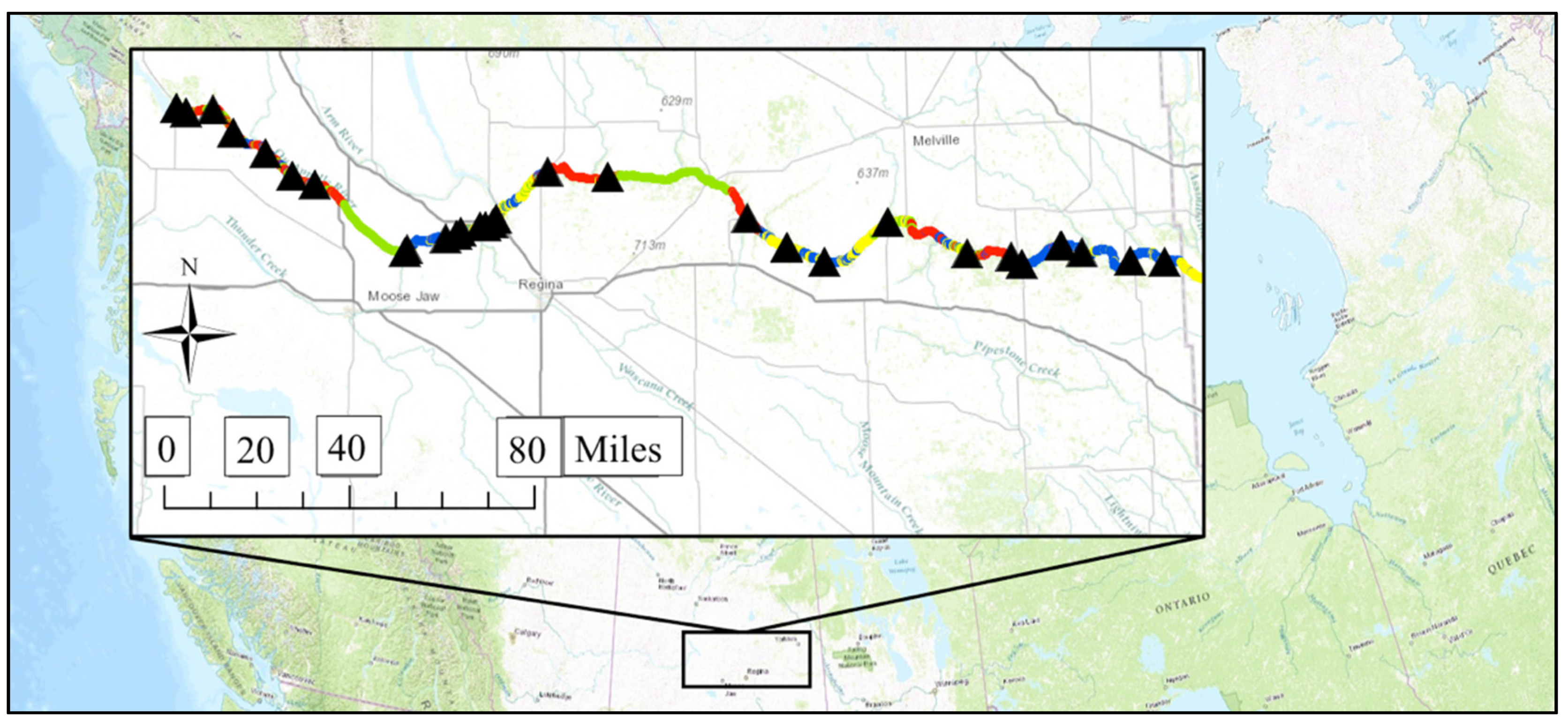
2.1. Study River

The Qu’Appelle River watershed is located in the Saskatchewan plains region of Canada, which encompasses many different topographical features such as ground moraines, lake plains, and river valleys [18]. The length of the river is 430 km, originating at the Qu’Appelle Dam at Lake Diefenbaker (located at 550m above sea level) and flowing into the Assiniboine River, just beyond the Manitoba-Saskatchewan boundary (Figure 1). The system contains a number of lakes, broad floodplains, and sweeping meanders. There are several existing threats to the sustainable functioning of the aquatic ecosystem, including disrupted flow regime, loss of connectivity, channelization, climate change, and amplified anthropogenic use. The watershed area contains industrial, urban, and agricultural development, resulting in an ever-increasing water demand [19]. Irrigation and potash mining are two main sources of increased water demand in the area, which will only intensify; together, these two activities could account for three-quarters of the water use in the river basin by 2060 [19]. For the environment, society, and economy of the Qu’Appelle area to thrive under these strains, long-term solutions must be found [19].

The gross drainage area of the Qu’Appelle River at the outlet station (Station #05JM001 near Welby) is 50,900 km². This station is just past the 35th and final macroinvertebrate sampling site used in this study, and is located at 394.57 m above sea level. Highest flows were 7 July 2014 at 454 m³/s, and flows have been as low as 0.0 m³/s, several times between 1987 and 1988, which were very low flow years. The average between 1974 and 2014 was 12 m³/s. The minimum stream width recorded at the centerline points was 6.8 m, the maximum was 2226.9 m, and the average was 168.7 m. The lowest monthly mean discharge at the station (1975–1993) happens in February (2.6 m³·s⁻¹) and the monthly mean discharge upsurges abruptly from March to April (3.7 to 17 m³·s⁻¹), resulting from the prairie snowmelt period [20]. Following the spring freshet, the monthly mean discharge declines abruptly, maintaining low levels throughout the remainder of the season with the exception of a minor upsurge in autumn, serving to draw down lake levels for the subsequent year’s spring runoff [20].

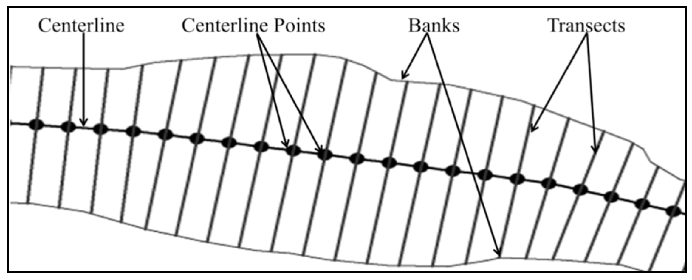
2.2. Creating the Geospatial Model

As the study focusses on the geospatial characteristics of the river, several characteristics (sinuosity, slope, fractal dimension, stream width) were chosen to be the points of comparison in the model. These characteristics were selected because they provide a satisfactory overview of the local fluvial geomorphology. The model has the potential to be expanded for other studies or in different river basins to include a variety of features, such as the average water temperature, dissolved oxygen concentration, depth, or flow. To create the geospatial model of the Qu’Appelle River, sinuosity, slope, fractal dimension, and stream width were extracted from a combination of Lidar (Water Security Agency) and 1:50,000 CanVec digital elevation model (DEM) data (Department of natural resources Canada), using Geographic Information System (GIS) software (ESRI 2013). Given the accessibility of this information to researchers, the model is flexible and could be completed for fluvial watersheds all over the world. A river polygon was first delineated, and a river centerline was added along the entire length of the river. Points were placed along the centerline at 50-meter intervals, followed by a transect (bank to bank) at each centerline point (Figure 2). Average bank point elevations were extracted from the DEM, and for each 50 m section, the river’s sinuosity, slope, fractal dimension and stream width could then be determined [10].

Sinuosity measures the intensity of river windiness and is defined as the ratio between the centerline length of a river stretch to the straight-lined distance between its endpoints [21,22,23]. Sinuosity can also be understood as a relationship between the slope of the valley to the slope of the river [23], or between the river length and valley length (shortest possible distance). Different terms are used to describe the spectrum of sinuosity values (S), including S = 1 for a straight-lined (linear) stretch, and in order of increasing sinuosity, elongated, oscillating, tortuous, and finally meandering with S > 2 [24,25]. Very sinuous rivers have a higher silt and clay content in their bed material [26], with S > 1.5 pointing to a riverbed consisting of over 92% fine textured material [23]. Sixty-three percent of the Qu’Appelle River’s stretch has a sinuosity of S > 1.5, suggesting that its bed has a balance of both coarse and fine materials, coinciding with the till blanket constituting most of the surficial geology of the Qu’Appelle River basin. Sinuosity in our study is the length of a river reach divided by the shortest distance between the reach end points, with a sinuosity score of 1 being a straight channel, and >1 a meandering one. The determination of a river’s sinuosity is an important goal, as the meandering of a system can influence sedimentation and various hydrological and ecological processes in the nearby environment [22].

The fractal dimension of a channel is a measurement of how much of the river length fills a certain Euclidean space. It is similar to sinuosity but quantifies an order of magnitude larger than sinuosity; it is indicative of the amplitude of meander change, within a river reach [21,27]. Fractal dimension can be helpful when examining complex meandering river patterns in the context of larger, geological viewpoints [10,22]. Both sinuosity and fractal dimension were calculated using the commercial software package Mathcad^® v.15 (Parametric Technology Corporation; PTC, Inc., Needham, MA, USA) [28]. Sinuosity was calculated at a slightly larger scale than width and slope, using 40 adjacent points (20 upstream and 20 downstream of each centerline point). Fractal dimension was calculated based on the number of centerline points that fell within a 40 km × 40 km square window moved along the course of the river. These scales were chosen because they were the values at which peak variation was calculated, giving the greatest range and, therefore, the most information about each variable. As described in Lindenschmidt and Long (2012), geomorphic typologies were identified by performing a Principal Component Analysis (PCA) of these four variables (sinuosity, slope, fractal dimension, stream width), using the statistical package R 2.15.2 [10,29]. The PCA was chosen because it is able to reduce the dimensionality of a data set with a large number of descriptors, and subsequently identify patterns within it [30]. The dataset of the four geomorphic characteristics calculated at each centerline point was log₁₀ + 1 transformed to improve normality while accounting for the high incidence of zeros and very small positive values. The explained variance of principal components (PC) one through four was 49%, 24%, 14% and 13%, respectively. Following Jolliffe’s (1972, 2002) modified Kaiser’s rule, the eigenvalues for components 3 and 4 were both less than 0.7 (0.57 and 0.52, respectively); therefore, only the first two principal components (accounting for 73% cumulative variance) were used to derive typologies [31,32]. The sum of binary values assigned to PCs at each centerline point, 1 for positive PC values and 0 for negative PC values, identified different geomorphic typologies, resulting in four unique geomorphic typologies (Figure 3).

River typologies were each given an identifying color and assigned to the corresponding 50-meter centerline points. Patterns within the typology distribution were visually assessed to identify spatial groupings (GRUs); eight different GRUs were identified along the Qu’Appelle River (Figure 3). An example of repetitive typology patterns being identified as a GRU occurs in GRU I, which is composed of Typology 1 and 3, as compared to GRU II that is a mix of typologies 0, 1 and 3 (Figure 3). As the objective of this study is to identify geomorphologically similar reaches along the river, GRUs were assigned to reaches that exhibited repetitive patterns in typology associations, separating such units in transition zones where large patterns gradually or abruptly changed (Figure 3).

2.3. Macroinvertebrate Sampling

Macroinvertebrate sampling was carried out prior to and separate from the delineation of GRUs, taking place between 2006 and 2009. With the GRU model, it would be ideal to delineate the geomorphological typologies before data collection instead, so that the sampling sites could be decided in light of the model and with a more even distribution amongst the GRUs. We collected benthic macroinvertebrate samples at a total of 35 sites along the Qu’Appelle River, from Lake Diefenbaker at its headwaters to its termination at its confluence with the Assiniboine River at the Manitoba border (Figure 1). Sites were selected for road access and with a pre-determined minimum 10 km river distance between sites. At each site, samples were collected in a 500 µm mesh d-frame net using a time and space standardized travelling kick and sweep (TK & S). This is a standardized method of sampling, which allows for the comparison of communities in similar habitats, between sites. Specifically, each sample comprised five evenly spaced positions along a transect from bank to opposite bank. These five samples were then integrated into one composite sample for each site. The transect sampled was perpendicular to the river channel and, at each position, an area ~30 cm × 30 cm was kicked to a depth of ~5 cm, for 10 s. In each collection, the net was swept downstream of the collector. All sites had similar features of straight, slow flowing reaches with no riffles. Substrate was typically soft silt, but did include small patches of cobble and vegetation on the bank positions. Ultimately, the objective of this study was to use a standardized method of benthic macroinvertebrate collection in comparable habitats across all sites, so that the dominant communities of the major habitat features would be represented. Although this method does not ensure that all taxa present at a site are represented, we feel we have adequately characterized the most dominant assemblages and habitat features.

All benthic macroinvertebrate samples were preserved in 80% ethanol in the field, and sorted from the organic material under 7× magnification in the laboratory. Benthic macroinvertebrates were identified to family designations using keys for North America [15] and western Canada where available [33,34,35]. Voucher series were deposited in both the Water Security Agency of Saskatchewan Invertebrate Voucher Collection (Saskatoon, Saskatchewan), and the Royal Saskatchewan Museum (Regina, Saskatchewan). Further, taxa occurrence records were submitted to the Saskatchewan Conservation Data Center with the Ministry of Environment.

2.4. EPT/C Ratio

Although many sensitive benthic macroinvertebrates can be found in water with organic pollution, polluted stretches are often dominated by Chironomidae and freshwater Oligochaeta worms [2]. Chironomids can thrive in a wide variety of habitats due to physical adaptations and high tolerance levels; as such, they are commonly held to be indicators of poor water quality [15,36]. Conversely, Ephemeroptera, Plecoptera, and Trichoptera (EPT) do not thrive in compromised water conditions due to their low pollution tolerance [6,14,37]. A high proportion of sensitive EPT at a site should therefore indicate higher water quality [38]. By comparing the population of EPT to that of Chironomidae, a metric of community health can be established for the site [38]. A habitat in good condition will have a more even distribution among these groups, rather than an overwhelming abundance of chironomids above EPT. Finding the sum of individual organisms in the Ephemeroptera, Plecoptera, and Trichoptera orders and dividing that total by the aggregate number of chironomids calculates an EPT/C ratio. A higher number is a positive result, meaning the chironomids are outnumbered by the EPT. A lower number shows possible environmental stress, as the EPT are greatly surpassed by chironomids.

2.5. Shannon Diversity Index

The Shannon diversity index is a biological index indicating biodiversity; this value increases as the number and distribution of taxa within the community increases [38]. As a measure of diversity, it includes both evenness and richness to evaluate community health [14]. A Shannon diversity index value was determined for each macroinvertebrate sample site in this study. The proportion of total biomass for each family was first determined within each sample site by dividing the total number of individuals in each family, by the total number of individuals of all the families together. The natural logarithm of each of these family proportion values was then found. The negative sum of these values for all families at a site represents its Shannon diversity index value. A higher Shannon diversity index value indicates a more diverse population, in this case at the family level, within the study site.

2.6. Family Biotic Index

An additional metric of ecosystem health commonly used to assess the impact of organic pollution, is the family biotic index (FBI) [39]. Hilsenhoff (1988) developed the index by designating tolerance values of organic pollution to benthic macroinvertebrates by family, ranging from 0 (very intolerant) to 10 (very tolerant) [38,39]. These values are based on family distribution in pollution; for instance, a family only found in pristine waters would be given a lower value like 0 or 1 [14]. Specifically, the number of benthic macroinvertebrates in each family is recorded, and then the FBI is calculated by multiplying the abundance per family by that family’s respective tolerance value. These family abundances adjusted to tolerance are then summed and divided by the total number of organisms in a sample and multiplied by 10. The resulting FBI value between 0 and 10 can indicate a level of water quality and corresponding degree of organic pollution present at the site (

Table 1. Biotic index scores and associated water quality in the Qu’Appelle River [38,39]. Far right column displays results from the 35 Qu’Appelle River sampling sites.

Biotic Index Score	Water Quality	Degree of Organic Pollution	Percent of Sites
0.00–3.50	Excellent	No apparent organic pollution	0% (0)
3.51–4.50	Very Good	Possible slight organic pollution	6% (2)
4.51–5.50	Good	Some organic pollution	31% (11)
5.51–6.50	Fair	Fairly significant organic pollution	34% (12)
6.51–7.50	Fairly Poor	Significant organic pollution	26% (9)
7.51–8.50	Poor	Very significant organic pollution	3% (1)
8.51–10.00	Very Poor	Severe organic pollution	0% (0)

) [39].

2.7. Comparing GRUs to Macroinvertebrate Data

Each of the macroinvertebrate indices (EPT/C, Shannon diversity index, family biotic index) were calculated separately for each sampling site. The data collected at each of the 35 macroinvertebrate sampling sites was sorted into the eight GRUs for comparison. Qualitative analysis of these results was carried out to identify any patterns. Separate from these indices, the macroinvertebrate community was combed through within each GRU at the family level, to pinpoint any family–GRU relationships. This study focused on the comparison of GRUs to family-level macroinvertebrate data only.

3. Results and Discussion

The purpose of the study is to complete an assessment of the GRU method applied to macroinvertebrate habitats, as a proof of concept. This is accomplished completely through desktop means, including the creation of the model to identify relationships between macroinvertebrates and GRUs. Therefore, our objective is to demonstrate the worth of the GRU model as a method of collecting useful geomorphological data, and as a tool to be applied to macroinvertebrate habitat in rivers. Our methods first detailed the making of the geospatial model and identification of the GRUs; these are further explained and discussed below. Once the model was created, the provided macroinvertebrate data are superimposed on the GRU network of the Qu’Appelle River. The standard macroinvertebrate indices described in the methods are completed and related within the parameters of GRUs, to reveal relationships between the macroinvertebrates and the GRUs. We hypothesize that GRUs will relate to some of the variation in macroinvertebrate community features as well as macroinvertebrate habitat selection.

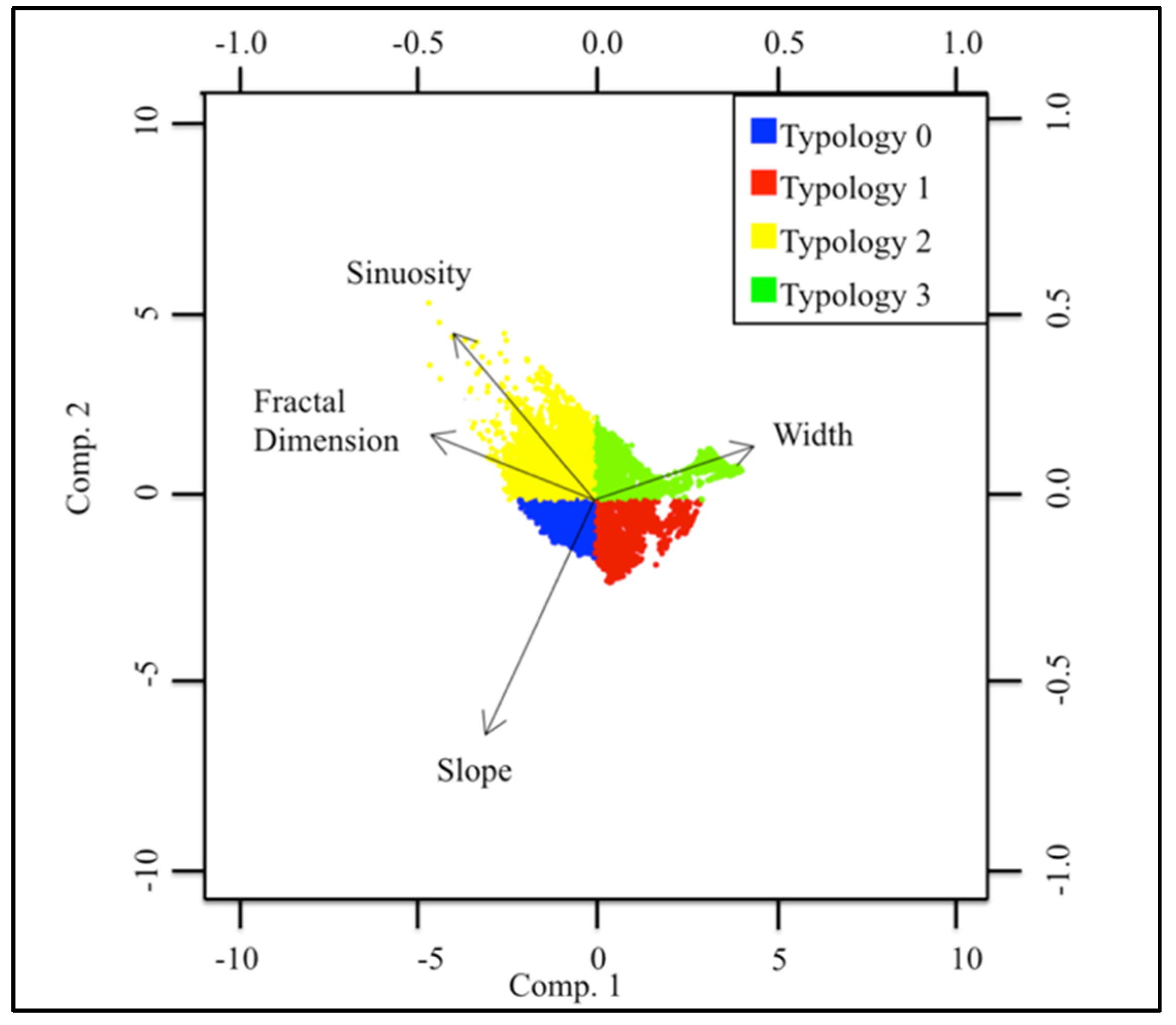
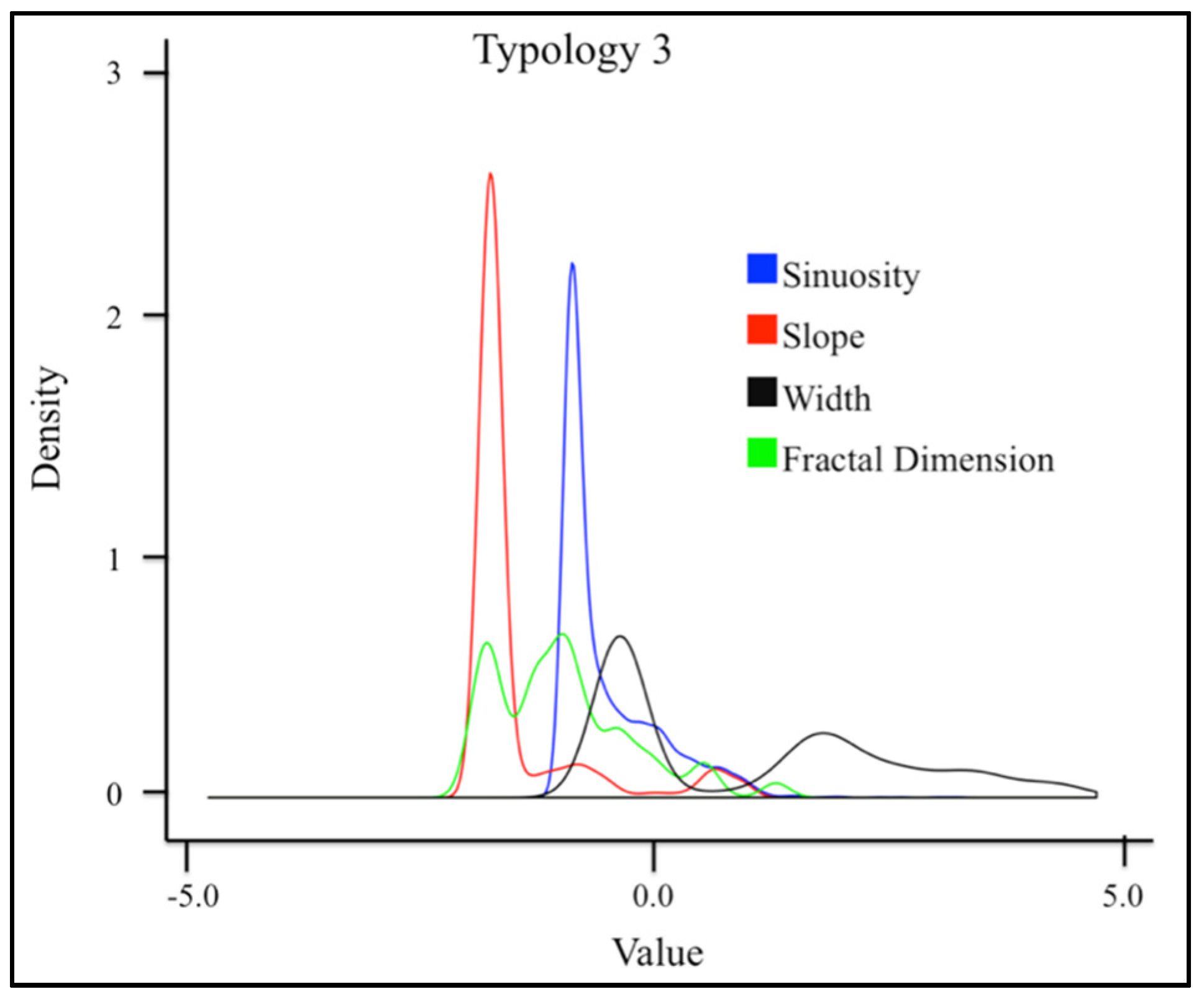
3.1. Geospatial Factors

Figure 4 shows PCA scores (color coded by typology) and variable vectors plotted in terms of principal component one on the x-axis, and component two on the y-axis. Principal components one and two account for 73% of the total variation in the dataset. In general, sinuosity and fractal dimensions tend to be more positively related to one another, while relationships between other variables differ depending on the typology of interest (Figure 4). General relationships between the four geomorphological variables (sinuosity, slope, fractal dimension, and channel width), as well as their relationships within different typologies, can be inferred from the biplot in Figure 4.

Density plots of normalized values of sinuosity, slope, fractal dimension, and channel width were also used to examine the qualitative contribution of each of these variables to each unique geomorphic typology based on absolute means (Figure 5).

General relationships for all four typologies are summarized in

Table 2. Qualitative contribution of variables to each typology derived from the Principal Component Analysis. (− is a negative relationship, + is a positive relationship, 0 is no discernable relationship).

Typology	Sinuosity	Slope	Fractal Dimension	Width
0	0	+	+	−
1	−	+	−	−
2	+	0	+	−
3	−	−	−	+

. Typology 0 is positively related to slope and fractal dimension and negatively related to width, implying more narrow regions of a higher fractal dimension and slope (Table 2). Typology 1 is positively related to slope but has a negative relationship with all other variables, associating it to narrow areas with a low fractal dimension and less meanders, and a high slope. (Table 2). Typology 2 is positively related to sinuosity and fractal dimension and negatively related to width, associated to highly sinuous and narrow reaches, with a high fractal dimension. Typology 3 has a negative relationship with all variables except width, meaning it is comprised of wide and straight reaches with low slope and fractal dimension values (Figure 4, Table 2).

The typologies were grouped into eight different GRUs, by identified patterns within the typology distribution (Figure 3).

Table 3. Summary of typology makeup, and the number of macroinvertebrate samples contained within each GRU.

GRU		I	II	III	IV	V	VI	VII	VIII
Typology Makeup	Most	1	1, 0, 3	3	3, 2	0	0, 2	1	2
	Other	3	-	-	1	1, 2, 3	3, 1	0, 2	0, 3
Macroinvertebrate Sample Sites		8	2	0	4	9	6	4	2

provides a summary of what these GRUs are composed of, as well as how many macroinvertebrate sites were available within each of them.

For example, GRU III is characterized by Typology 3 exclusively, which is positively related to stream width (Table 2 and Table 3). Correspondingly, the GRU consists of large water bodies (i.e., Buffalo Pound Lake, Pasqua Lake, Echo Lake, Mission Lake) within which no macroinvertebrate data was collected (Table 3, Figure 3). Some of the smaller reservoirs (i.e., Eyebrow Lake, Katepwa Lake, Crooked Lake, Round Lake) are not a part of this GRU.

3.2. Overall Macroinvertebrate Indices Results

The three macroinvertebrate indices used here (EPT/C ratio, Shannon diversity index, family biotic index) were chosen because they are often used in macroinvertebrate community evaluations. Upon calculating the indices for each of the 35 sampling sites, it became clear that variation from site to site was high, and relationships to the GRUs were minimal. As a result, the focus shifted towards macroinvertebrate family distribution, as a more qualitative evaluation. The results of all three macroinvertebrate indices are recorded and displayed graphically below. The relationships discovered between specific macroinvertebrate families and GRUs are also detailed below.

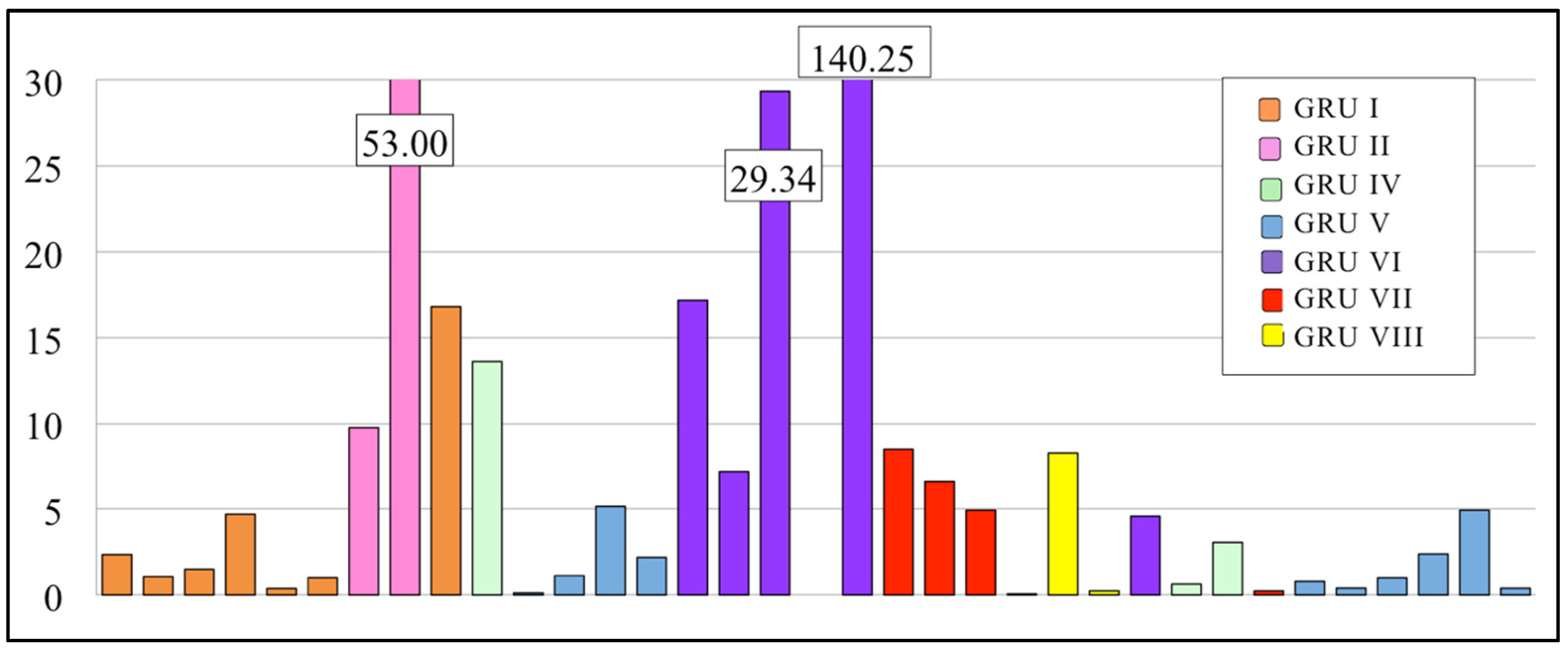
3.2.1. EPT/C Ratio

Minor relationships can be observed between the GRUs and the EPT/C ratio results; for instance, some of the highest EPT/C scores were recorded in GRU VI. GRU I and GRU V have lower average EPT/C ratios than other regions. However, the site to site variation is undeniable, and no obvious patterns can be identified.

GRU I has an average EPT/C of 3.48 (Figure 6). GRU II has an average EPT/C of 31.38, GRU IV has an average EPT/C of 4.35, and the average EPT/C ratio in GRU V is 2.04. GRU VI has an average EPT/C of 33.09 and 39.71 without site 53. The lowest EPT/C score was calculated at Site 53, with a ratio of 0 (0 EPT and 3 chironomids; Figure 7). GRU VII has an average EPT/C of 5.07. GRU VIII has an average EPT/C ratio of 4.25.

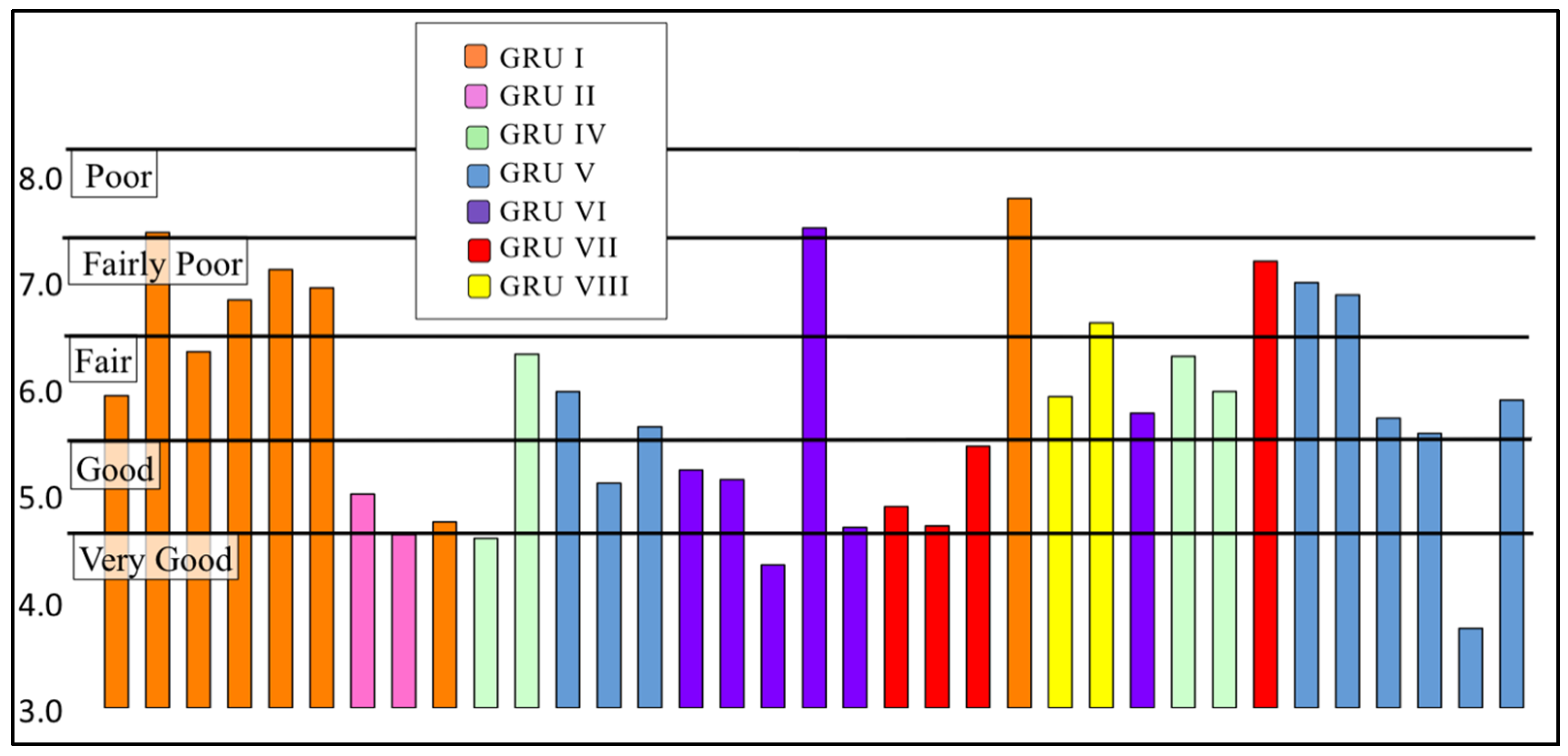
3.2.2. Family Biotic Index

Similar to the EPT/C results, the high variation between sites hinders our ability to pinpoint specific GRU patterns in this analysis. GRU I has the worst average results in the family biotic index analysis. GRU VI generally seems to have the best average, aside from the two sites contained in GRU II. GRU I has an average biotic index value of 6.64 (fairly poor; Table 1, Figure 7). GRU II has an average biotic index value of 4.82 (good), GRU IV has an average biotic index value of 5.79 (fair), and GRU V has an average biotic index value of 5.72 (fair). GRU VI has an average biotic index value of 5.44 (good), and 5.03 (good) without site 53. Site 53 received the second-worst biotic index value of 7.50. GRU VII has an average biotic index value of 5.56 (fair), and GRU VIII has an average biotic index value of 6.27 (fair). The undeniable disparity of FBI scores between sites as opposed to between GRUs points to the necessity of including local influences (i.e., agriculture, industry) in future studies.

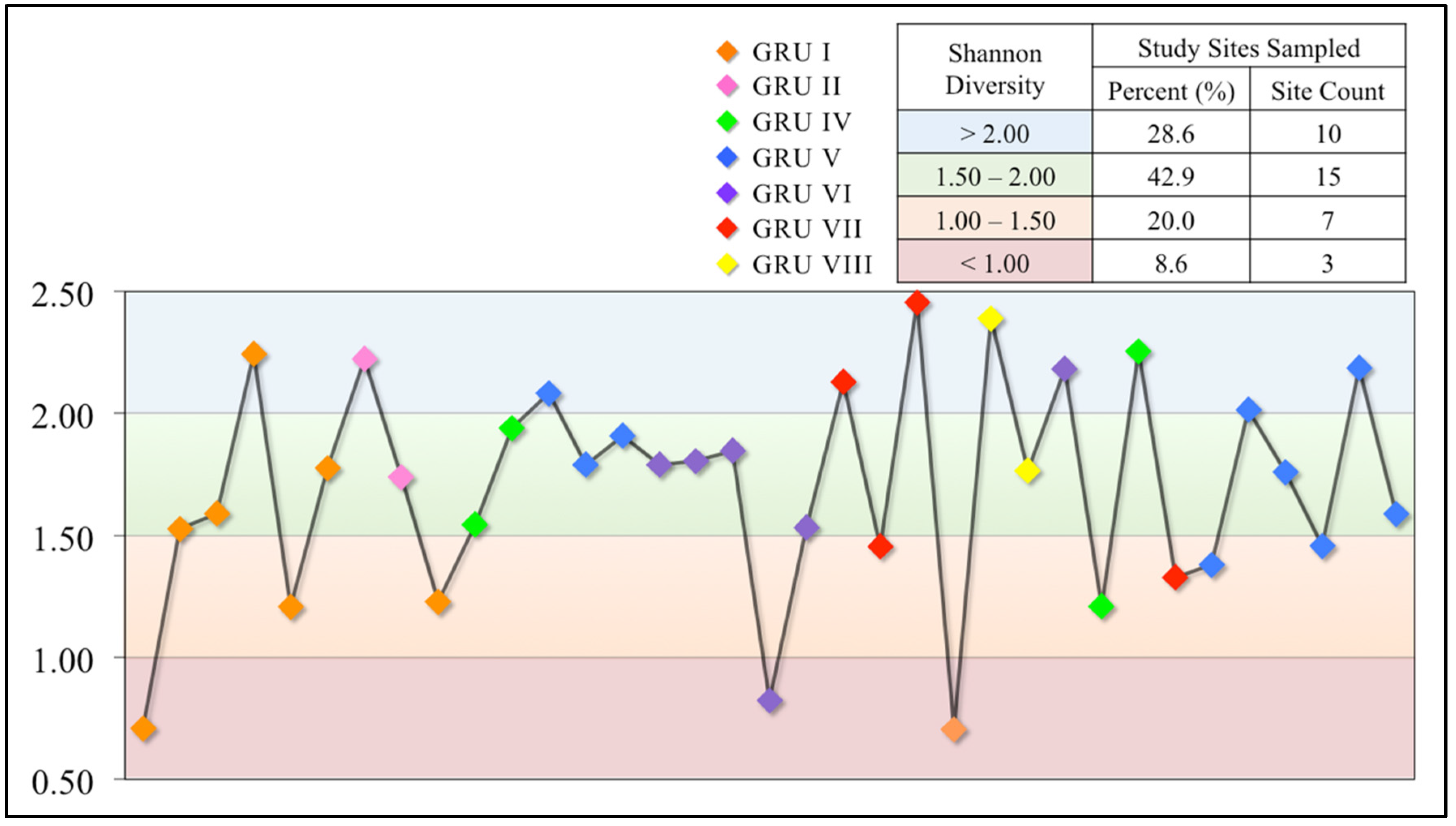
3.2.3. Shannon Diversity Index

The Shannon diversity values found in this study ranged from 0.71 to 2.46. As with the other macroinvertebrate indices, most of the GRUs do not show an obvious relationship to the Shannon diversity index. For instance, the sites within GRU V all fall within similar Shannon diversity ranges, whereas GRU I contains a high variety of results. Studies with a more even site distribution amongst GRUs may obtain more useful Shannon diversity results.

GRU I has an average Shannon diversity score of 1.37 (Figure 8). GRU II has an average Shannon diversity of 1.98, GRU IV has an average Shannon diversity of 1.74, and GRU V has an average Shannon diversity of 1.80. GRU VI has an average Shannon diversity of 1.66 and 1.83 without site 53. Site 53, within GRU VI, received the penultimate Shannon diversity score of only 0.82. GRU VII has an average Shannon diversity of 1.84, and GRU VIII has an average Shannon diversity of 2.08.

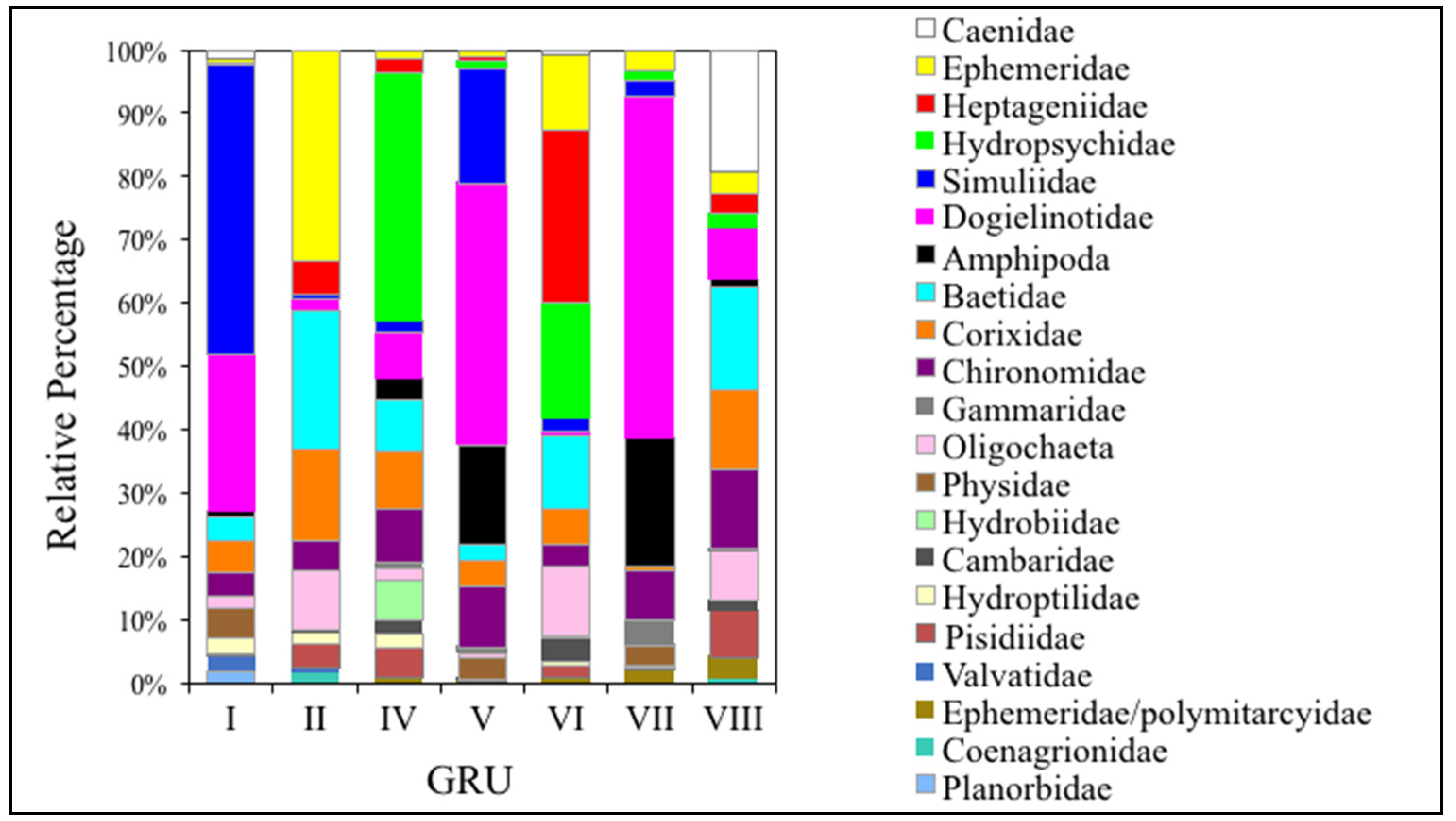
3.3. Comparing GRUs to Macroinvertebrate Data

Overall community makeup shifts highly from site to site; the lowest total individuals recorded was 12 at site 53 and the highest was 40,227 at site 35. The complete data set contains 115,696 individuals from 63 families. The initial qualitative examination of this vast data set was accomplished through examining the family abundance within each GRU. The westernmost stretch of the Qu’Appelle River, immediately downstream of Lake Diefenbaker, consists mainly of GRUs I and II (Figure 3). All of the GRU I sites contain Chironomidae, Corixidae, and Oligochaeta. Most (6/7) sites also contain Dogielinotidae, which is the second highest family by relative percentage for GRU I (Figure 9). The family Simuliidae (black fly larvae) had the highest abundance in GRU I. Both GRU II sites contain Baetidae, Cambaridae, Chironomidae, Coenagrionidae, Corixidae, Ephemeridae, Heptageniidae, Hydroptilidae, Oligochaeta, and Pisidiidae. The highest abundance in GRU II is the family Ephemeridae, followed by Baetidae, Corixidae, and Oligochaeta. GRU IV occurs in 5 relatively small stretches throughout the river (Figure 3). Each of these sites contain Oligochaeta, and the families Chironomidae, Ephemeridae, Cambaridae, and Pisidiidae. The most abundant family in GRU IV is Hydropsychidae; following this family by abundance are Corixidae, Chironomidae, and Baetidae.

GRU V appeared throughout the river. All nine sites within GRU V contain Chironomidae and Dogielinotidae, and most (8/9) contain Baetidae and Heptageniidae. The most abundant family in GRU V is the Dogielinotidae, followed by Simuliidae, and those identified only to the Amphipoda order. Besides site 53, all five other sites within GRU VI contain the families Cambaridae, Chironomidae, Corixidae, Ephemeridae, Heptageniidae, and those identified as being in the Oligochaeta class. The most abundant family is Heptageniidae, followed by Hydropsychidae, Baetidae, Ephemeridae, and Oligochaeta. Site 53, within GRU VI, contains the smallest total, at only 12 individuals, eight of which were the aquatic worm taxa Oligochaeta, which is known to be highly tolerant to adverse environments and is often used as an indicator of polluted systems [14]. This site also has a family richness of only 3; besides the aforementioned Oligochaeta (only identified to class), it contains just Corixidae and Chironomidae. All four sites within GRU VII contain the families Chironomidae, Corixidae, Hydropsychidae, and Pisidiidae. The most abundant family is Dogielinotidae, followed by those only identified as Amphipoda. GRU VIII is made up of three small reaches, all in the eastern half of the Qu’Appelle River, and two sample sites. Both sites contain the families Caenidae, Cambaridae, Chironomidae, Corixidae, Ephemeridae, Gammaridae, Heptageniidae, Hydropsychidae, Leptoceridae, Notonectidae, Physidae, Pisidiidae, and Dogielinotidae. The most abundant family in GRU VIII is the Caenidae, followed by Baetidae (Figure 9). Due to the vastness of the data set, simply observing the relative abundance by GRU did not point to any obvious significant relationships. However, through comparing the family abundance within each GRU, certain families stood out as important within the system. The qualitative examination, seeking relationships between the GRUs and macroinvertebrate families, continued then by focusing on certain family distributions.

3.3.1. EPT Families

Hydropsychidae net-spinner caddisflies compose 2.38% of the total population (the sum of individuals within all sampling sites) with 2748 individuals (

Table A1. Qu’Appelle River macroinvertebrate taxa list, including order, family, functional feeding group, and count.

Qu’Appelle River Macroinvertebrate Taxa List
Order	Family	Functional Feeding Groups	Total	Order	Family	Functional Feeding Groups	Total
Acari	Acari	Predators	15	Gastropoda	Ancylidae	Scrapers	14
Amphipoda	Amphipoda	Collector Gatherers	14269.91		Gastropoda	Scrapers	1
	Gammaridae	Collector Gatherers	2046.05		Hydrobiidae	Scrapers	165
	Dogielinotidae	Collector Gatherers	44289.81		Lymnaeidae	Scrapers	140
Total			60605.76		Physidae	Scrapers	3825.57
Coleoptera	Dytiscidae	Predators	106		Planorbidae	Scrapers	506
	Elmidae	Collector Gatherers	122.82		Valvatidae	Scrapers	643
	Gyrinidae	Predators	70	Total			5294.57
	Haliplidae	Shredders	43	Hemiptera	Corixidae	Herbivores	3021.56
	Hydraenidae	Scrapers	4			Predators	586.02
	Hydrophilidae	Collector Gatherers	10		Notonectidae	Predators	14
		Herbivores	1	Total			3621.58
		Predators	1	Hydrachnidia	Hydrachnidia	Predators	53
		Shredders	1	Lepidoptera	Crambidae	Herbivores	546
Total			358.82		Lepidoptera	Herbivores	10
Collembola	Collembola	Collector Gatherers	1		Noctuidae	Herbivores	264
Decopoda	Cambaridae	Omnivores	166	Total			820
Diptera	Athericidae	Predators	2	Malacostraca	Cambaridae	Omnivores	257
	Ceratopogonidae	Predators	167.04	Nematoda	Nematoda	Predators	15
	Chironomidae	Collector Gatherers	7747.06	Odonata	Coenagrionidae	Predators	165
		Predators	442.26		Gomphidae	Predators	16
	Diptera	Collector Gatherers	18		Lestidae	Predators	16
	Empididae	Predators	39	Total			197
	Leptoceridae	Shredders	22	Oligochaeta	Oligochaeta	Detritivores	1514.70
	Simuliidae	Filterers	19958	Ostracoda	Ostracoda	Filterers	8
	Stratiomyidae	Collector Gatherers	1	Pelecypoda	Pisidiidae	Filterers	691.10
	Tabanidae	Predators	12	Pharyngobdellida	Erpobdellidae	Predators	24
	Tipulidae	Predators	10	Plecoptera	Perlidae	Predators	5
Total			28418.35		Plecoptera	Shredders	1
					Pteronarcyidae	Shredders	10
				Total			16
Ephemeroptera	Baetidae	Scrapers	3088.10	Rhynchobdellida	Glossiphoniidae	Predators	20
	Caenidae	Collector Gatherers Scrapers	491
		Filterers	279
	Ephemeridae	Collector Gatherers	2666.82	Trichoptera	Brachycentridae	Filterers	238
	Ephemeridae/polymitarcyidae	Collector Gatherers	891		Hydropsychidae	Filterers	2748.02
	Ephemeroptera	Scrapers	353.27		Hydroptilidae	Herbivores	770
	Heptageniidae	Collector Gatherers	437		Leptoceridae	Collector Gatherers	54
		Scrapers	1189.82			Herbivores	16
	Isonychiidae	Filterers	4			Shredders	92.02
	Leptohyphidae	Collector Gatherers	79		Phryganeidae	Shredders	31.02
	Leptophlebiidae	Collector Gatherers	52.85		Polycentropodidae	Filterers	8
		Scrapers	2			Predators	20
	Polymitarcyidae	Collector Gatherers	82		Trichoptera	Shredders	6
Total			9615.86	Total			3983.05
Grand Total							115695.80

). They have tolerance levels of 4 or 5. They are filterers and clingers, preferring lotic environments. These caddisflies spin nets to catch food (organic matter) in flowing water [6]. Physical adaptations allow them to attach to stones and stabilize themselves in swift currents [15]. These lotic insects prefer more rapid water flow, as it aids in food collection [5]. Sedimentation can cause tearing or burying of their nets, or can cause the nets to get clogged, both of which lessens food capture and increases energy expenditure [40,41]. They have been found to be especially intolerant of fine substrates near agricultural sites and could therefore be used as indicators of habitat degradation as a result of increased sedimentation [5]. Few of these Hydropsychidae are found in GRUs I, II, and VIII. Totals range between 0 and 21 individuals; however, they are fairly evenly distributed throughout the rest of the GRUs (IV, V, VI, VII), ranging from 401 to 885 individuals, even ranking as the most abundant family in GRU IV (Figure 9). The limited representation of Hydropsychidae in these GRUs seems to indicate the presence of an unsuitable habitat for them. In comparing only the GRUs and the macroinvertebrate data in this instance, perhaps the lack of Hydropsychidae in GRUs I, II, and VIII could be due to increased suspended sediment, unsuitable for their catchnet-method of food collection. This could be further collaborated in future studies that include sediment data, local land use information, and water chemistry data.

GRU VII contains many burrowing families, including the majority of the Ephemeridae/ Polymitarcyidae burrowing mayflies (775/891). It also contains almost half (1316/2667) the population of the burrowing mayfly family Ephemeridae, designated with a tolerance level of 6. This family selects finer sediments in which to build tunnels, such as soft, firm clay or clay-silt [41,42]. It can cope with low oxygen levels by beating its gills to create a current through its burrow [2]. Sand, gravel, and detritus stemming from leaves and twigs are unsuitable for this mayfly’s burrowing [42]. Sometimes, stream currents disturb and mix the sediments, which has been known to interfere with maintenance of Ephemeridae burrows [42]. All four sample sites within GRU IV contain Ephemeridae, as well as 5/6 (excluding site 53) in GRU VI. The comparison of GRUs to macroinvertebrate family data in this case indicates that GRU VII must have a habitat compatible with burrowing families. Perhaps, the sediment common in GRU VII is finer, such as silt or clay, and not sand. This could be further confirmed in future second-tier studies that include field data, such as water and sediment, as well as information about regional terrestrial practices.

All the Plecoptera (stoneflies) are found in GRU V, at the two sample sites farthest east. One of these, the stonefly Pteronarcyidae, is the only species found to have the lowest tolerance of 0. Likewise, the other stoneflies were found to be sensitive, with an assigned tolerance of 1. Stoneflies are generally associated with low pollution, well-oxygenated, healthy running water, and are therefore useful in water quality and biotic integrity analyses [14]. GRU V also contains all of certain Trichoptera and Ephemeroptera families. One of the most sensitive Trichoptera families, Brachycentridae, is exclusively found in GRU V. It is a filterer preferring the lotic environment, with a tolerance of 1. It also contains all of two Ephemeroptera families, Leptohyphidae (tolerance 4) and Leptophlebiidae (tolerance 2). Through the comparison of GRU and macroinvertebrate family data only, it can be inferred that GRU V is a fairly healthy environment. It contains many sensitive species, and scored fairly well in the macroinvertebrate population indices. Further studies, including additional data, and more specific species data, could further corroborate this.

3.3.2. Dipteran Families

The Dipteran black fly larva family Simuliidae appears at only 4/8 sites in GRU I, yet this GRU contains the majority (12,573/19,958) of this family and it ranked as the most abundant family of the GRU (Figure 9). A total of 6086 Simuliidae are found in GRU V, and 1153 in GRU VII. The bulk of these individuals in GRU I are found at the first sample site (Site 45; 12,236 individuals), immediately downstream of Lake Diefenbaker. These black fly larvae have a tolerance of 6, and comprise 15.67% of the total benthic macroinvertebrate population sampled here. Black fly larva are not selective consumers, and can adapt to selective pressures [41,43]. They spread silk webs to attach to substrate, stones or vegetation, for stabilization in currents, and motility [15]. These adaptations also include a wide range of behaviors such as those for avoiding predators, moving across substratum, and adapting to different flow conditions [43]. They are most often found on rocks, submerged wood, and stream bottom substrates, preferring relatively clean surfaces to which they can stick and remain stationary [41,44]. The disturbance of the Diefenbaker dam right before site 45 could explain the dominance of this insensitive family; however, this hypothesis needs further data to be validated. This cannot be attributed as a GRU characteristic, as the extremely high abundance of Simuliidae was only found at Site 45.

A large number of Chironomidae midges (used in EPT/C) were collected in GRUs V (3260) and VII (3358). A total of 8189 Chironomidae were in the sample (Table A1). As burrowers, they often prefer the finer sediment in which tunnels can be formed [41]. In general, these taxa can survive in diverse habitats; the larvae are not atmospheric respirators, so they can live in large deep waters [15]. As their sensitivity of 6–8 indicates, chironomids can often withstand low oxygen levels and organic pollution [38]. GRUs V and VII have fairly good EPT/C scores and Shannon diversity scores; however, the large number of Chironomidae may be affecting them in some instances. Dominance of Chironomidae is generally a negative indication of population health; more specific taxa information, as to what type of Chironomidae are comprising these numbers, could aid in determining the condition of these GRUs.

3.3.3. Lepidopteran Families

All 820 individuals in the order Lepidoptera were found within GRUs I and II. Lepidoptera were obtained in six out of 10 sample sites within GRUs I and II. The Lepidoptera were identified as either juvenile Grass Moths (family: Crambidae) or Owlet Moths (family: Noctuidae). Crambidae have been found to be polyphagous, meaning they feed on more than four different species of plant within at least three families [45]. Lepidopterans presiding in fluvial systems commonly graze on diatoms and periphyton [14]. They are believed to be more influenced by abiotic factors, such as food availability and geomorphology, than by biotic factors, such as trophic interactions and competition, in regards to their community structure and habitat selection [45]. The presence of these families exclusively in the first GRUs could be an indication of high plant presence, which could be substantiated in future studies that include more location-specific data. In lieu of this data, through the comparison of GRUs to macroinvertebrate family data only, the presence of Lepidopterans as indicators of stable macrophyte habitat can be further corroborated by other herbivorous species being abundant in these GRUs as well. In fact, these first typologies also contain nearly all (642/643) snails in the family Valvatidae. Consistent with the herbivorous Crambidae and Noctuidae, Valvatidae snails have been found to prefer high vegetative cover and diversity of floating vegetation. These snails rely on gills for gas exchange and are vulnerable to anoxia [46]. GRUs I and II also contain 674/770 representatives of the caddisfly family Hydroptilidae, found in 5/10 sites. Hydroptilidae case-building caddisflies are herbivores, with a tolerance level of 4, mainly feeding on periphyton or dead leaves [14]. They both feed on and use filamentous algae to build their cases [5]. The indication of stable macrophyte coverage and a relationship between these GRUs and herbivorous families shows a link between the model and macroinvertebrate habitat distribution.

3.3.4. Amphipoda Families

GRU VII contains 33,646/60,606 Amphipoda, and Site 35 (GRU VII) contains 33,637 of them. This site also has half of the total amphipod family Dogielinotidaein the sample; these have a high organic pollution tolerance of 8. Due to their often-high abundance, Dogielinotidaeare commonly used as test organisms in toxicology studies [14]. They are an important food source for fish, waterfowl, salamanders, and large invertebrates [47]. Site 35 houses a majority of the amphipod family Gammaridae as well. GRU V contains 19,524/60,606 Amphipoda and, within it, Site 39 (GRU V) contains 16,928 of them. Site 35 is situated directly downstream from the Round Lake reservoir and Site 39 is the next site downstream, which could factor into the dominance of Amphipoda at these sites. The dominance of Amphipoda at site 39 could be caused by drift from Site 35. A future study including local influences, such as reservoirs, could aid in further verifying this hypothesis and revealing more about the health of sites 35 and 39. Again, this finding points more to site variation than GRU relationships.

4. Conclusions

The GRU method has functioned in revealing similar geomorphological stretches along the Qu’Appelle River (Figure 8). Taxa were related to the geomorphic typologies delineated in this study. Applying GRUs in benthic macroinvertebrate habitat identification has proven to be a difficult task. Relationships between the GRUs and macroinvertebrate distribution were challenging to find, given the high site to site variation recorded. Part 1 of the study yielded more significant results than Part 2. Although direct relationships between the GRUs and macroinvertebrates were minimal, the GRU model presents valuable geomorphological information. It provides a rapid and visual method to assess any unique river basin, by classifying the river into similar geomorphological characteristics. Subsequently, the GRUs further classify them into clusters and patterns in geomorphology. This process provides a sound basis and starting point for any number of studies. It provides a useful reference point to lead informed studies as well as to monitor any future shifts in local geomorphology. The findings within the study reported here could be used to design a more effective study in the future. The delineation of GRUs before sampling (as was not done in this study) could provide a more even sampling site distribution, and more even data collected for each GRU. The GRU model has the potential to be an effective tool to use while managing fluvial systems, and better developing field sampling campaigns. The use of the GRU model saves time and money because it can efficiently categorize river reaches, and can greatly improve the process of selecting sample sites. The findings recorded here indicate the need for additional data to be combined with the GRU model. The GRUs could be the primary step in evaluating the river, with subsequent steps including additional field data, and local influences. The delineation of the typologies themselves could include additional geospatial characteristics, to provide even more information to researchers.

The efforts demonstrated in this study were intended to use macroinvertebrate indices as a proof of concept of the GRU model. The study succeeded in showing that instream habitats can be pinpointed and related to the GRUs, but the GRUs proved to be too large to capture the high variability of the macroinvertebrate community. The GRU model has worked well in relation to more mobile fish species [11,12,13], but GRUs may be too coarse a resolution for the more sessile macroinvertebrate population. Part 1 of the series focused on the typology scale, which seemed to be a better fit for macroinvertebrates [17]. Future second tier studies should be able to substantiate the effectiveness of using GRUs to identify benthic macroinvertebrate habitat by further relating the two through a more comprehensive study. Such an analysis may consider the inclusion of river depth, sediment, vegetation, and local influences (i.e., nearby reservoirs, industry, municipalities). Studies could also focus on geomorphic typologies as related to macroinvertebrates, rather than the clustered GRUs, as was carried out in Part 1. Additional studies may also consider comparing these geospatial factors to more specific macroinvertebrate data, identified to genus or species. We recognize the fact that more data, collected in line with the GRU model and after it has been delineated, would be a great asset and aid in the quality of analysis. The highly dynamic nature of both the river and macroinvertebrate community make it difficult to create a simple method to link the GRUs to the macroinvertebrates. The Qu’Appelle River will further be studied with a water quality model currently being developed to provide water temperatures and dissolved oxygen concentrations at the centerline points used in the model. Through doing so, the objective is to find a practical and useful way to use the macroinvertebrate data discussed here, in light of geomorphology and climate change. This has been purely a desktop study comparing macroinvertebrate family data to GRUs; the desktop research is well suited as a basis for future studies to further understand the Qu’Appelle River system. Additionally, these findings reveal potential for the GRU model to be applied to other river systems as an efficient resource management method. The use of GRUs can be a valuable precursor for more detailed habitat studies. Through categorizing fluvial systems by geomorphological characteristics, GRUs can provide insight into instream habitat complexity, availability, and connectivity as a whole.

References

- D’Ambrosio, J.L.; Williams, L.R.; Witter, J.D.; Ward, A. Effects of Geomorphology, Habitat, and Spatial Location on Fish Assemblages in a Watershed in Ohio, USA. Environ. Monit. Assess. 2009, 148, 325–341. [Google Scholar] [CrossRef] [PubMed]
- Allan, J.D.; Castillo, M.M. Stream Ecology; Springer Science & Business Media: Dordrecht, The Netherlands, 2007. [Google Scholar]
- Rodríguez-Iturbe, I.; Valdés, J.B. The Geomorphologic Structure of Hydrologic Response. Water Resour. Res. 1979, 15, 1409–1420. [Google Scholar] [CrossRef]
- Dollar, E.S.J.; James, C.S.; Rogers, K.H.; Thoms, M.C. A Framework for Interdisciplinary Understanding of Rivers as Ecosystems. Geomorphology 2007, 89, 147–162. [Google Scholar] [CrossRef]
- Chakona, A.; Phiri, C.; Day, J. Potential for Trichoptera Communities as Biological Indicators of Morphological Degradation in Riverine Systems. Hydrobiologia 2008, 621, 155–167. [Google Scholar] [CrossRef]
- O’Laughlin, K. The Streamkeeper’s Field Guide: Watershed Inventory and Stream Monitoring Methods; Adopt-a-Stream Foundation: Washington, DC, USA, 1996. [Google Scholar]
- Dufrêne, M.; Legendre, P. Species Assemblages and Indicator Species: The Need for a Flexible Asymmetrical Approach. Ecol. Monogr. 1997, 67, 345–366. [Google Scholar] [CrossRef]
- Kubosova, K.; Brabec, K.; Jarkovsky, J.; Syrovatka, V. Selection of Indicative Taxa for River Habitats: A Case Study on Benthic Macroinvertebrates Using Indicator Species Analysis and the Random Forest Methods. Hydrobiologia 2010, 651, 101–114. [Google Scholar] [CrossRef]
- Bovee, K.D.; Lamb, B.L.; Bartholow, J.M.; Stalnaker, C.B.; Taylor, J.; Henriksen, J. Stream Habitat Analysis Using the Instream Flow Incremental Methodology; U.S. Geological Survey, Biological Resources Division Information and Technology Report: Fort Collins, CO, USA, 1998.
- Lindenschmidt, K.E.; Long, J. A GIS Approach to Define the Hydro-Geomorphological Regime for Instream Flow Requirements Using Geomorphic Response Units (GRU). River Syst. 2013, 20, 261–275. [Google Scholar] [CrossRef]
- Carr, M.K.; Lacho, C.; Pollock, M.; Watkinson, D.A.; Lindenschmidt, K.-E. Development of geomorphic typologies for identifying Lake Sturgeon (Acipenser fulvescens) habitat in the Saskatchewan River System. River Syst. 2015, 21, 215–227. [Google Scholar] [CrossRef]
- Carr, M.K.; Watkinson, D.A.; Svendsen, J.C.; Enders, E.C.; Long, J.M.; Lindenschmidt, K.-E. Geospatial modeling of the Birch River: Distribution of Carmine Shiner (Notropis percobromus) in Geomorphic Response Units (GRU). Int. Rev. Hydrobiol. 2015, 100, 129–140. [Google Scholar] [CrossRef]
- Carr, M.K.; Watkinson, D.A.; Lindenschmidt, K.-E. Identifying links between Fluvial Geomorphic Response Units (FGRU) and fish species in the Assiniboine River, Manitoba. Ecohydrology 2016. [Google Scholar] [CrossRef]
- Dodds, W.K.; Whiles, M.R. Freshwater Ecology: Concepts and Environmental Applications of Limnology; Academic Press: San Diego, CA, USA, 2010. [Google Scholar]
- Merritt, R.W.; Cummins, K.W.; Hunt, K. An Introduction to the Aquatic Insects of North America; Kendall/Hunt Publishing Company: Dubuque, IA, USA, 1996. [Google Scholar]
- Ernst, A.G.; Warren, D.R.; Baldigo, B.P. Natural–Channel–Design Restorations That Changed Geomorphology Have Little Effect on Macroinvertebrate Communities in Headwater Streams. Restor. Ecol. 2012, 20, 532–540. [Google Scholar] [CrossRef]
- Meissner, A.G.N.; Carr, M.K.; Phillips, I.D.; Lindenschmidt, K-E. Using a Geospatial Model to Relate Fluvial Geomorphology to Macroinvertebrate Habitat in a Prairie River—Part 1: Genus-Level Relationships with Geomorphic Typologies. Water 2016, 8, 42. [Google Scholar] [CrossRef]
- Mollard, J.D. Morphological Study of the Upper Qu’Appelle River; Friends of Wascana Marsh: Regina, SK, Canada, 2004. [Google Scholar]
- Clifton Associates Ltd. Upper Qu’Appelle Water Supply Project: Economic Impact and Sensitivity Analysis; Report to Water Security Agency; Clifton Associates Ltd.: Regina, SK, Canada, 2012. [Google Scholar]
- Pomeroy, J.; de Boer, D.; Martz, L. Hydrology and Water Resources of Saskatchewan: Centre for Hydrology Report #1; University of Saskatchewan: SK, Canada, 2005. [Google Scholar]
- Shen, X.H.; Zou, L.J.; Zhang, G.F.; Su, N.; Wu, W.Y.; Yang, S.F. Fractal Characteristics of the Main Channel of Yellow River and Its Relation to Regional Tectonic Evolution. Geomorphology 2011, 127, 64–70. [Google Scholar] [CrossRef]
- Güneralp, İ.; Abad, J.D.; Zolezzi, G.; Hooke, J. Advances and Challenges in Meandering Channels Research. Geomorphology 2012, 163–164, 1–9. [Google Scholar] [CrossRef]
- Ahnert, F. Einführung in Die Geomorphologie; Verlag Eugen Ulmer: Stuttgart, Germany, 2015. [Google Scholar]
- Lüderitz, V.; Kunz, C.; Wüstemann, O.; Remy, D.; Feuerstein, B. Typisierung und Bewertung für die leitbildorientierte Sanierung von Altwässern. In Flussaltwässer: Ökologie und Sanierung; Lüderitz, V., Langheinrich, U., Kunz, C., Eds.; Vieweg + Teubner: Wiesbaden, Germany, 2009; pp. 91–168. [Google Scholar]
- Zumbroich, T.; Müller, A. Das Verfahren der Gewässerstrukturkartierung. In Strukturgüte von Fließgewässern: Grundlagen und Kartierung, 1st ed.; Zumbroich, T., Müller, A., Günther, F., Eds.; Springer-Verlag Berlin Heidelberg: Berlin, Germany, 1999; pp. 97–121. [Google Scholar]
- Schumm, S.A. The Fluvial System; John Wiley & Sons: New York, NY, USA, 1977; p. 338. [Google Scholar]
- Schuller, D.J.; Rao, A.R.; Jeong, G.D. Fractal Characteristics of Dense Stream Networks. J. Hydrol. 2001, 243, 1–16. [Google Scholar] [CrossRef]
- MathSoft Inc. Mathcad v.15; MathSoft Inc.: Cambridge, MA, USA, 2012. [Google Scholar]
- R Development Core Team. R: A Language and Environment for Statistical Computing; R Foundation for Statistical Computing: Vienna, Austria, 2012; Available online: https://www.r-project.org/ (accessed on 10 September 2015).
- Legendre, P.; Legendre, L. Numerical Ecology, 3rd ed.; Elsevier: Amsterdam, The Netherlands, 2012. [Google Scholar]
- Jolliffe, I.T. Discarding Variables in a Principal Component Analysis. I: Artificial Data. J. R. Stat. Soc. C (Appl. Stat.) 1972, 21, 160–173. [Google Scholar] [CrossRef]
- Jolliffe, I.T. Principal Component Analysis, 2nd ed.; Springer: New York, NY, USA, 2002; p. 488. [Google Scholar]
- Dosdall, L.M.; Lehmkuhl, D.M. Stoneflies (Plecoptera) of Saskatchewan. Quaest. Entomol. 1979, 15, 3–116. [Google Scholar]
- Clifford, H.F. Aquatic Invertebrates of Alberta; The University of Alberta Press: Edmonton, AB, Canada, 1991. [Google Scholar]
- Webb, J.M. The Mayflies of Saskatchewan. Master’s Thesis, University of Saskatchewan, Saskatoon, SK, Canada, 2002. [Google Scholar]
- Berg, M.B.; Hellenthal, R.A. The Role of Chironomidae in Energy Flow of a Lotic Ecosystem. Netherland J. Aquat. Ecol. 1992, 26, 471–476. [Google Scholar] [CrossRef]
- Karaus, U.; Larsen, S.; Guillong, H.; Tockner, K. The Contribution of Lateral Aquatic Habitats to Insect Diversity along River Corridors in the Alps. Landsc. Ecol. 2013, 28, 1755–1767. [Google Scholar] [CrossRef]
- Mandaville, S.M. Benthic Macroinvertebrates in Taxa Tolerance Values, Metrics, and Protocols; Project H–1; Soil and Water Conservation Society of Metro Halifax: Halifax, NS, Canada, 2002. [Google Scholar]
- Hilsenhoff, W.L. Rapid Field Assessment of Organic Pollution with a Family-Level Biotic Index. J. North Am. Benthol. Soc. 1988, 7, 65–68. [Google Scholar] [CrossRef]
- Strand, R.M.; Merritt, R.W. Effects of Episodic Sedimentation on the Net- Spinning Caddisflies Hydropsyche betteni and Ceratopsyche Sparna (Trichoptera: Hydropsychidae). Environ. Pollut. 1998, 98, 129–134. [Google Scholar] [CrossRef]
- Jones, J.I.; Murphy, J.F.; Collins, A.L.; Sear, D.A.; Naden, P.S.; Armitage, P.D. The Impact of Fine Sediment on Macroinvertebrates. River. Res. Appl. 2012, 28, 1055–1071. [Google Scholar] [CrossRef]
- Krieger, K.A.; Bur, M.T.; Ciborowski, J.J.H.; Barton, D.R.; Schloesser, D.W. Distribution and Abundance of Burrowing Mayflies (Hexagenia Spp.) in Lake Erie 1997–2005. J. Great Lakes Res. 2007, 33, 20–33. [Google Scholar] [CrossRef]
- Eymann, M. Flow Patterns Around Cocoons and Pupae of Black Flies of the Genus Simulium (Diptera: Simuliidae). Hydrobiologia 1991, 215, 223–229. [Google Scholar] [CrossRef]
- Eymann, M.; Friend, W.G. Behaviors of Larvae of the Black Flies Simulium vittatum and S. decorum (Diptera: Simuliidae) Associated with Establishing and Maintaining Dispersion Patterns on Natural and Artificial Substrates. J. Insect. Behav. 1988, 1, 169–186. [Google Scholar] [CrossRef]
- Stoops, C.A.; Adler, P.H.; McCreadie, J.W. Ecology of Aquatic Lepidoptera (Crambidae: Nymphulinae). Hydrobiologia 1998, 379, 33–40. [Google Scholar] [CrossRef]
- Watson, A.M.; Ormerod, S.J. The Distribution of Three Uncommon Freshwater Gastropods in the Drainage Ditches of British Grazing Marshes. Biol. Conserv. 2004, 118, 455–466. [Google Scholar] [CrossRef]
- Government of Canada Fisheries and Oceans. Manual for the Culture of Selected Freshwater Invertebrates; Lawrence, S.G., Ed.; Department of Fisheries and Oceans Freshwater Institute: Winnipeg, MB, Canada, 1981. [Google Scholar]