
Modeling the Impact of Ditch Water Level Management on Stream–Aquifer Interactions


Abstract
:1. Introduction
2. Methods
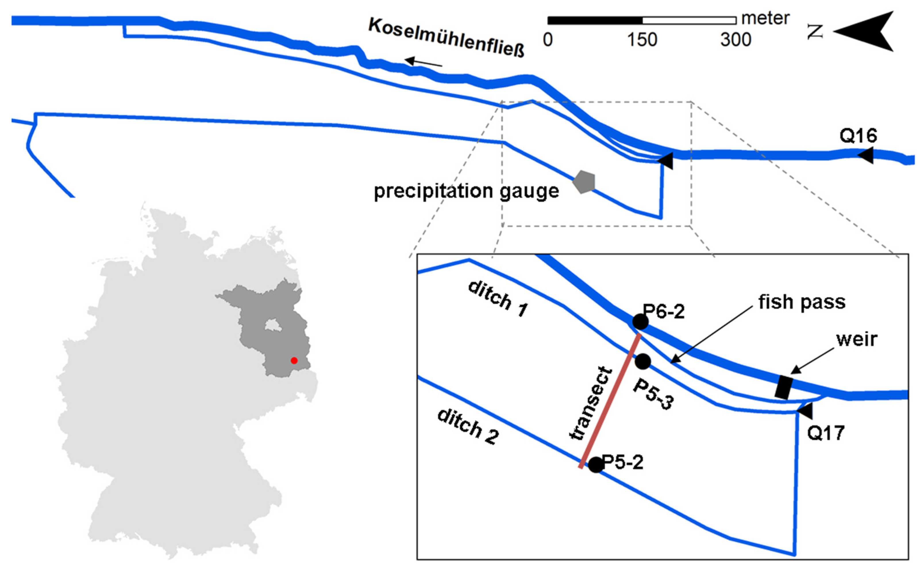
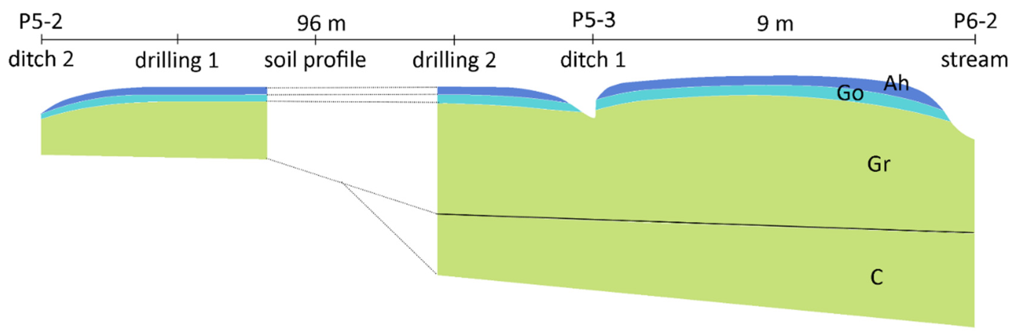
2.1. Study Site
2.2. Data
2.3. Modeling Framework
2.3.1. Model Set-Up
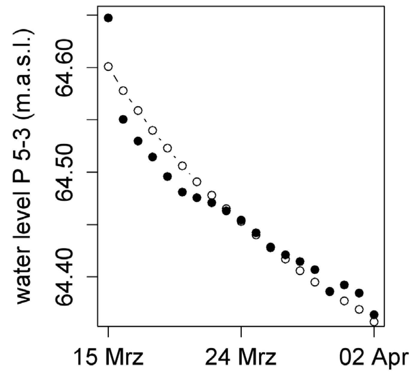
2.3.2. Model Calibration and Validation
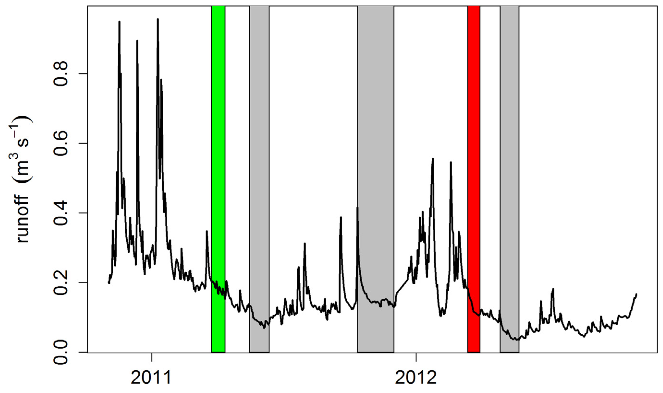
2.4. Scenarios
3. Results
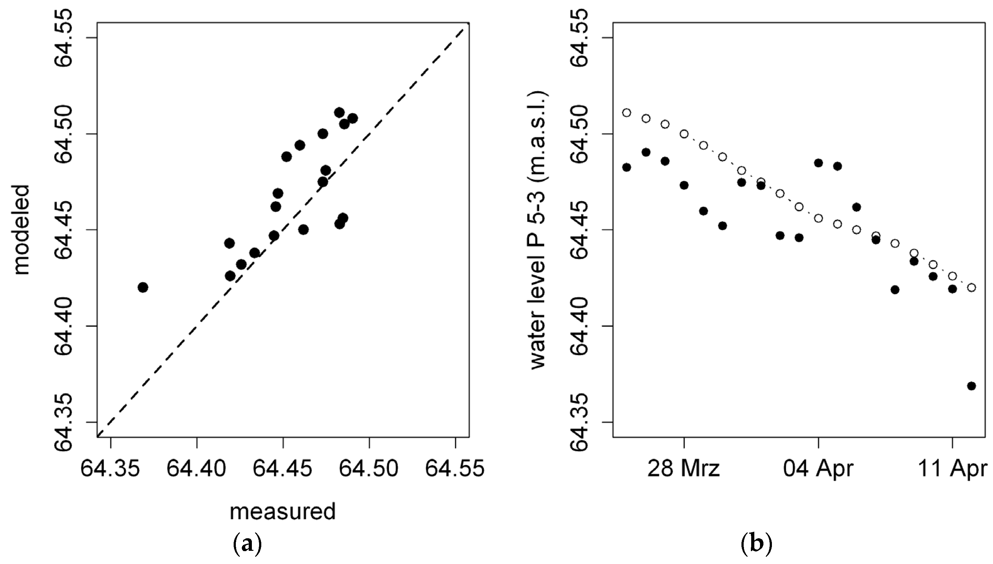
3.1. Model Calibration and Validation
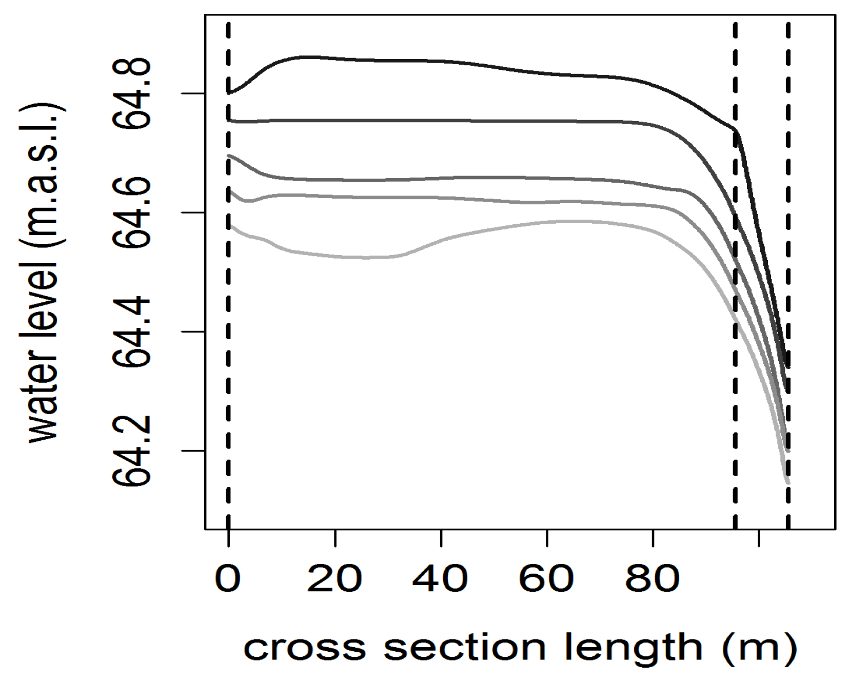
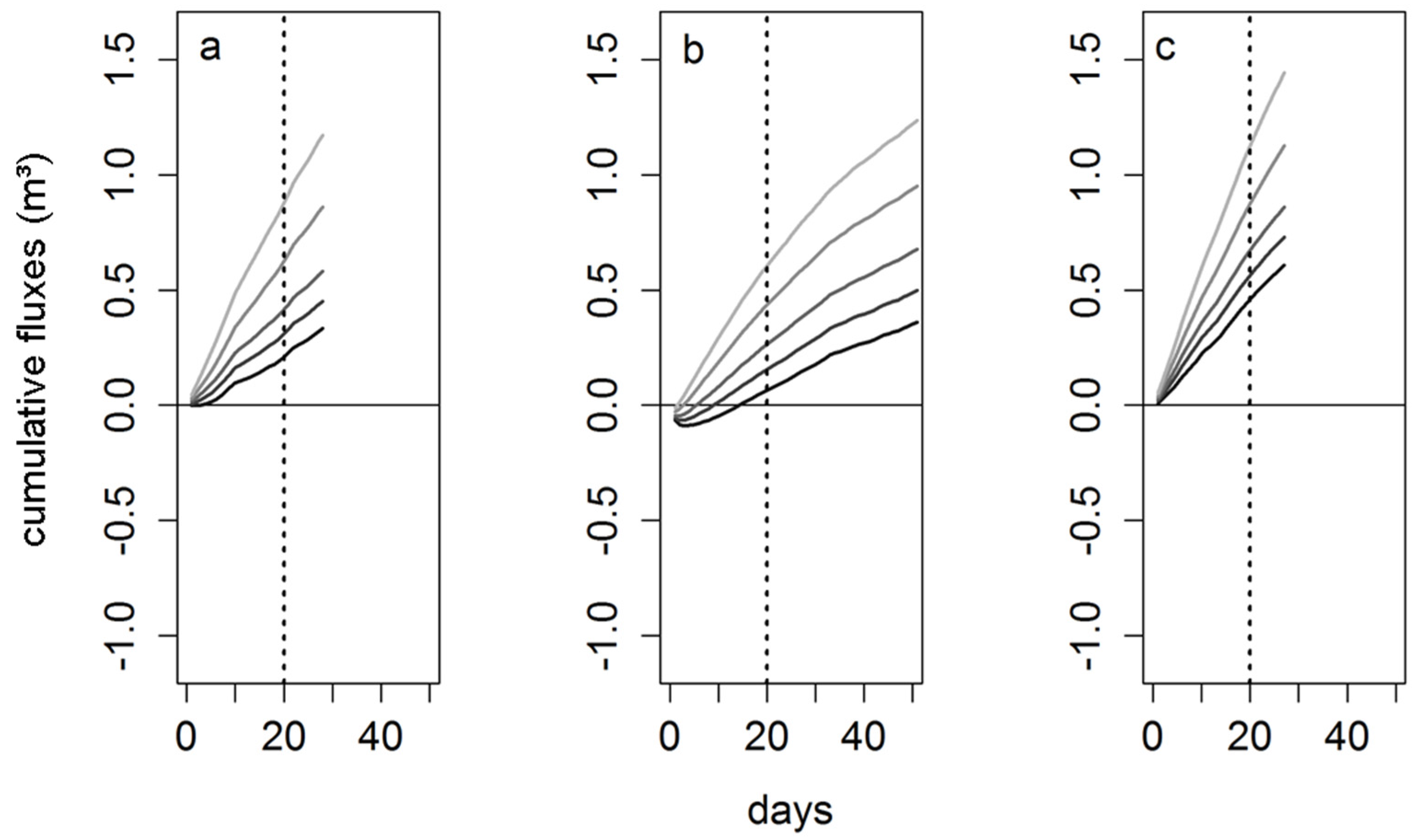
3.2. Scenario Results
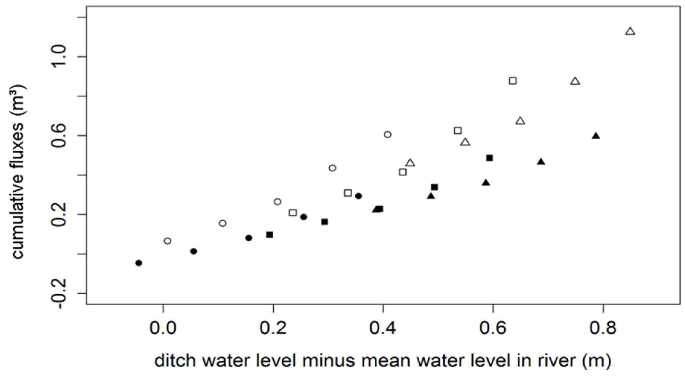
3.3. Water Balance of Low Flow Periods
4. Discussion
5. Conclusions
Acknowledgments
Author Contributions
Conflicts of Interest
References
- Pandey, D.N.; Gupta, A.K.; Anderson, D.M. Rainwater harvesting as an adaptation to climate change. Curr. Sci. 2003, 85, 46–59. [Google Scholar]
- Solomon, S.; Qin, D.; Manning, M.; Chen, Z.; Marquis, M.; Averyt, K.B.; Tignor, M.; Miller, H.L. Climate Change 2007: The Physical Science basis. Contribution of Working Group i to The Fourth Assessment Report of The Intergovernmental Panel on Climate Change. Summary for Policymakers; Cambridge University Press: Cambridge, UK, 2007; pp. 339–378. [Google Scholar]
- Postel, S.L. Entering an era of water scarcity: The challenges ahead. Ecol. Appl. 2000, 10, 941–948. [Google Scholar] [CrossRef]
- Conradt, T.; Koch, H.; Hattermann, F.; Wechsung, F. Spatially differentiated management-revised discharge scenarios for an integrated analysis of multi-realisation climate and land use scenarios for the elbe river basin. Reg. Environ. Chang. 2012, 12, 633–648. [Google Scholar] [CrossRef]
- Wegehenkel, M.; Kersebaum, K.C. A first assessment of the impact of climate change on discharge and groundwater recharge in a catchment in northeastern germany. J. Agrometeorol. 2008, 10, 274–281. [Google Scholar]
- Taylor, R. Rethinking water scarcity: The role of storage. Eos Trans. Am. Geophys. Union 2009, 90, 237–248. [Google Scholar] [CrossRef]
- Kinal, J.; Stoneman, G.L. Disconnection of groundwater from surface water causes a fundamental change in hydrology in a forested catchment in south-western australia. J. Hydrol. 2012, 472–473, 14–24. [Google Scholar] [CrossRef]
- Thomas, B.; Lischeid, G.; Steidl, J.; Dannowski, R. Regional catchment classification with respect to low flow risk in a pleistocene landscape. J. Hydrol. 2012, 475, 392–402. [Google Scholar] [CrossRef]
- Thomas, B.; Steidl, J.; Dietrich, O.; Lischeid, G. Measures to sustain seasonal minimum runoff in small catchments in the mid-latitudes: A review. J. Hydrol. 2011, 408, 296–307. [Google Scholar] [CrossRef]
- Dietrich, O. The Spreewald Integration Concept and Results on Water Balance Developments. In Integrated Analysis of The Impacts of Global Change on Environment and Society in The Elbe River Basin; Weißensee-Verl.: Berlin, Germany, 2008; pp. 266–275. [Google Scholar]
- Dietrich, O.; Steidl, J.; Pavlik, D. The impact of global change on the water balance of large wetlands in the Elbe lowland. Reg. Environ. Chang. 2012, 12, 701–713. [Google Scholar] [CrossRef]
- Querner, E.P.; van Lanen, H.A.J. Impact assessment of drought mitigation measures in two adjacent dutch basins using simulation modelling. J. Hydrol. 2001, 252, 51–64. [Google Scholar] [CrossRef]
- Barber, M.E.; Hossain, A.; Covert, J.J.; Gregory, G.J. Augmentation of seasonal low stream flows by artificial recharge in the spokane valley-rathdrum prairie aquifer of idaho and washington, USA. Hydrogeol. J. 2009, 17, 1459–1470. [Google Scholar] [CrossRef]
- Konyha, K.D.; Shaw, D.T.; Weiler, K.W. Hydrologic design of a wetland—Advantages of continuous modeling. Ecol. Eng. 1995, 4, 99–116. [Google Scholar] [CrossRef]
- Sophocleous, M. Interactions between groundwater and surface water: The state of the science. Hydrogeol. J. 2002, 10, 52–67. [Google Scholar] [CrossRef]
- Sophocleous, M. The science and practice of environmental flows and the role of hydrogeologists. Ground Water 2007, 45, 393–401. [Google Scholar] [CrossRef] [PubMed]
- Nützmann, G.; Mey, S. Model-based estimation of runoff changes in a small lowland watershed of north-eastern germany. J. Hydrol. 2007, 334, 467–476. [Google Scholar] [CrossRef]
- Furman, A. Modeling coupled surface–subsurface flow processes: A review. Vadose Zone J. 2008, 7, 741–756. [Google Scholar] [CrossRef]
- Stanley, E.H.; Jones, J.B. Surface-Subsurface Interactions: Past, Present, and Future. In Streams and Ground Waters; Academic Press: San Diego, CF, USA, 2000; pp. 405–417. [Google Scholar]
- Twarakavi, N.K.C.; Šimůnek, J.; Seo, S. Evaluating interactions between groundwater and vadose zone using the hydrus-based flow package for modflow. Vadose Zone J. 2008, 7, 757–768. [Google Scholar] [CrossRef]
- Howard, K.F.; Maier, H.S.; Mattson, S.L. Ground-Surface Water Interactions and The Role of The Hyporheic Zone. In Groundwater and Ecosystems; Baba, A., Howard, K.F., Gunduz, O., Eds.; Springer: Berlin, Germany, 2006; Volume 70, pp. 131–143. [Google Scholar]
- Dietrich, O.; Redetzky, M.; Schwärzel, K. Wetlands with controlled drainage and sub-irrigation systems—modelling of the water balance. Hydrol. Process. 2007, 21, 1814–1828. [Google Scholar] [CrossRef]
- Abbasi, F.; Feyen, J.; van Genuchten, M.T. Two-dimensional simulation of water flow and solute transport below furrows: Model calibration and validation. J. Hydrol. 2004, 290, 63–79. [Google Scholar] [CrossRef]
- Gärdenäs, A.I.; Šimůnek, J.; Jarvis, N.; van Genuchten, M.T. Two-dimensional modelling of preferential water flow and pesticide transport from a tile-drained field. J. Hydrol. 2006, 329, 647–660. [Google Scholar] [CrossRef]
- Kandelous, M.M.; Šimůnek, J. Numerical simulations of water movement in a subsurface drip irrigation system under field and laboratory conditions using hydrus-2d. Agric. Water Manag. 2010, 97, 1070–1076. [Google Scholar] [CrossRef]
- Rassam, D.; Werner, A. Review of Groundwater–Surfacewater Interaction Modelling Approaches and Their Suitability for Australian Conditions; eWater Technical Report; eWater Cooperative Research Centre: Canberra, Australia, 2008; pp. 1–52. [Google Scholar]
- Germer, S.; Kaiser, K.; Bens, O.; Hüttl, R.F. Water balance changes and responses of ecosystems and society in the Berlin-Brandenburg region—A review. Die Erde 2011, 142, 65–95. [Google Scholar]
- Bullock, A.; Acreman, M. The role of wetlands in the hydrological cycle. Hydrol. Earth Syst. Sci. Discuss. 2003, 7, 358–389. [Google Scholar] [CrossRef]
- AG Boden. Bodenkundliche Kartieranleitung (English: Manual of Soil Mapping. 5th Ed. (KA5)), 5th ed.; Schweizerbart’sche Verlagsbuchhandlung: Stuttgart, Germany, 2005; p. 438. [Google Scholar]
- Richter, D. Ergebnisse methodischer Untersuchungen zur Korrektur des systematischen Messfehlers des Hellmann-Niederschlagsmessers; Deutscher Wetterdienst: Offenbach am Main, Germany, 1995. [Google Scholar]
- Wendling, U.; Schellin, H.G.; Thomä, M. Bereitstellung von täglichen Informationen zum Wasserhaushalt des Bodens für die Zwecke der agrarmeteorologischen Beratung. Z. Meteorol. 1991, 41, 468–475. [Google Scholar]
- German Meteorological Service. Available online: www.dwd.de (accessed on 6 March 2016).
- Schindler, U.; Durner, W.; von Unold, G.; Müller, L. Evaporation method for measuring unsaturated hydraulic properties of soils. Soil Sci. Soc. Am. J. 2010, 74, 1071–1083. [Google Scholar] [CrossRef]
- UMS GmbH. User Manual Hyprop; UMS GmbH: Munich, Germany, 2012. [Google Scholar]
- Van Genuchten, M.T. A closed-form equation for predicting the hydraulic conductivity of unsaturated soils. Soil Sci. Soc. Am. J. 1980, 44, 892–898. [Google Scholar] [CrossRef]
- Mualem, Y. New model for predicting hydraulic conductivity of unsaturated porous-media. Water Resour. Res. 1976, 12, 513–522. [Google Scholar] [CrossRef]
- Šimůnek, J.; van Genuchten, M.T.; Šejna, M. The Hydrus Software Package for Simulating Two- and Three Dimensional Movement of Water, Heat, and Multiple Solutes in Variably-Saturated Media; Technical Manual, Version 2.0; Pc Progress: Prague, Czech Republic, 2012; p. 258. [Google Scholar]
- Šimůnek, J.; van Genuchten, M.T.; Šejna, M. Development and applications of the hydrus and stanmod software packages and related codes. Vadose Zone J. 2008, 7, 587–600. [Google Scholar] [CrossRef]
- Vogel, H.J.; Ippisch, O. Estimation of a critical spatial discretization limit for solving Richards’ equation at large scales. Vadose Zone J. 2008, 7, 112–114. [Google Scholar] [CrossRef]
- Peters, A.; Durner, W. Simplified evaporation method for determining soil hydraulic properties. J. Hydrol. 2008, 356, 147–162. [Google Scholar] [CrossRef]
- Durner, W.; Jansen, U.; Iden, S.C. Effective hydraulic properties of layered soils at the lysimeter scale determined by inverse modelling. Eur. J. Soil Sci. 2008, 59, 114–124. [Google Scholar] [CrossRef]
- Feddes, R.A.; Kowalik, P.J.; Zaradny, H. Simulation of Field Water Use and Crop Yield; Centre for Agricultural Publishing and Documentation: Wageningen, The Netherlands, 1978. [Google Scholar]
- Sutanto, S.J.; Wenninger, J.; Coenders-Gerrits, A.M.J.; Uhlenbrook, S. Partitioning of evaporation into transpiration, soil evaporation and interception: A comparison between isotope measurements and a hydrus-1d model. Hydrol. Earth Syst. Sci. Discuss. 2012, 16, 2605–2616. [Google Scholar] [CrossRef]
- Wesseling, J.; Elbers, J.; Kabat, P.; van den Broek, B. Swatre: Instructions for Input. In Internal Note; Winand Staring Centre: Wageningen, The Netherlands, 1991. [Google Scholar]
- Taylor, S.A.; Ashcroft, G.M. Physical Edaphology. In The Physics of Irrigated and Nonirrigated Soils; Freeman and Co.: San Francisco, CA, USA, 1972; pp. 434–435. [Google Scholar]
- State Office for Mining, Geology and Raw Material of Brandenburg. Hydrogeologic Map of Brandenburg. Available online: http://www.geo.brandenburg.de/hyk50 (accesed on 3 March 2016).
- Stahl, K.; Hisdal, H.; Hannaford, J.; Tallaksen, L.M.; van Lanen, H.A.J.; Sauquet, E.; Demuth, S.; Fendekova, M.; Jodar, J. Streamflow trends in Europe: Evidence from a dataset of near-natural catchments. Hydrol. Earth Syst. Sci. Discuss. 2010, 14, 2367–2382. [Google Scholar] [CrossRef]
- State Office for Environment, Health and Consumer Protection of the Federal State of Brandenburg. Flächendeckende Modellierung von Wasserhaushaltsgrößen für das Land Brandenburg (English: Water Balance Modelling Across the Whole Area of the Federal State of Brandenburg); State Office for Environment, HACP: Potsdam, Germany, 2000. [Google Scholar]


| Horizon | eBD | Gravel | Sand | Silt | Clay | Textural class |
|---|---|---|---|---|---|---|
| (g·cm−3) | (%) | (%) | (%) | (%) | ||
| Ah | 1.18 | 1.8 (1.8) | 95.1 (1.8) | 2.9 (1.0) | <0.1 | Pure sand |
| Go | 1.77 | 1.6 (0.8) | 95.6 (0.8) | 2.2(1.6) | <0.1 | Pure sand |
| Gr | 1.91 | 6.2 (3.3) | 93.6 (3.3) | 0.3 (0.2) | <0.1 | Pure sand |
| C | - | 2.1 | 84.9 | 13.0 | <0.1 | Slightly silty sand |
| Horizon | Confidence Intervals | θr (-) | θs (-) | α (cm−1) | n (-) | Ks (cm·day−1) | l (-) |
|---|---|---|---|---|---|---|---|
| Ah | 2.5% | 0.120 | 0.540 | 0.0135 | 1.26 | 12.11 | |
| mean | 0.198 | 0.546 | 0.0167 | 1.38 | 21.82 | 0.5 | |
| 97.5% | 0.275 | 0.551 | 0.0206 | 1.58 | 39.32 | ||
| Go | 2.5% | −0.032 | 0.329 | 0.0203 | 1.29 | 5.11 | |
| mean | 0.024 | 0.333 | 0.0239 | 1.40 | 8.27 | 0.5 | |
| 97.5% | 0.080 | 0.337 | 0.0281 | 1.54 | 13.39 | ||
| Gr | 2.5% | −0.006 | 0.274 | 0.0245 | 1.99 | 4.88 | |
| mean | 0.000 | 0.278 | 0.0257 | 2.05 | 6.28 | 0.5 | |
| 97.5% | 0.006 | 0.282 | 0.0274 | 2.12 | 8.10 |
| Value | Calibration | Validation | Scenario Analyses | ||
|---|---|---|---|---|---|
| 15 March–2 April 2012 | 3 March–2 April 2011 | 16 May–12 June 2011 | 12 October–1 December 2011 | 26 April–22 May 2012 | |
| P (mm) | 5 | 10 | 18 | 11 | 14 |
| pET (mm) | 39 | 42 | 117 | 39 | 95 |
| initial WLS (m a.s.l.) | 64.25 | 64.37 | 64.28 | 64.62 | 64.11 |
| min WLS (m a.s.l.) | 64.02 | 64.22 | 64.05 | 64.25 | 63.79 |
| Scenario | P | ETa | Stream | Ditch 2 | Ditch 1 | ∆S | MWatBalR |
|---|---|---|---|---|---|---|---|
| (mm·day−1) | (mm·day−1) | (mm·day−1) | (mm·day−1) | (mm·day−1) | (mm·day−1) | (%) | |
| (a) 16 May–12 June 2011 | Initial Stream Water Level: | 64.28 m a.s.l. | |||||
| 10cm | 0.31 | 4.12 | 0.10 | −3.29 | 0.00 | −0.62 | 0.07 |
| 20 cm | 0.31 | 4.13 | 0.15 | −3.49 | 0.00 | −0.47 | 0.06 |
| 30 cm | 0.31 | 3.87 | 0.20 | −2.50 | 0.00 | −1.25 | 0.02 |
| 40 cm | 0.31 | 3.11 | 0.30 | −1.99 | 0.00 | −1.12 | 0.07 |
| 50 cm | 0.31 | 2.28 | 0.42 | −1.02 | 0.00 | −1.36 | 0.47 |
| baseline | 0.31 | 3.69 | 0.16 | −0.09 | −0.98 | −2.48 | 0.18 |
| (b) 12 October–1 December 2011 | Initial Stream Water Level: | 64.63 m a.s.l. | |||||
| 10 cm | 0.42 | 0.86 | 0.03 | 1.13 | 0.00 | −1.60 | 0.06 |
| 20 cm | 0.42 | 0.81 | 0.07 | 0.85 | 0.00 | −1.31 | 0.05 |
| 30 cm | 0.42 | 0.73 | 0.13 | 0.44 | 0.00 | −0.87 | 0.03 |
| 40 cm | 0.42 | 0.59 | 0.21 | 0.33 | 0.00 | −0.71 | 0.13 |
| 50 cm | 0.42 | 0.46 | 0.29 | 0.04 | 0.00 | −0.36 | 0.10 |
| baseline | 0.42 | 0.45 | 0.33 | 0.07 | −0.30 | −0.13 | 0.25 |
| (c) 26 April–22 May 2012 | Initial Stream Water Level: | 64.11 m a.s.l. | |||||
| 10 cm | 0.86 | 3.28 | 0.22 | −2.42 | 0.00 | −0.22 | 0.06 |
| 20 cm | 0.86 | 3.29 | 0.27 | −2.53 | 0.00 | −0.17 | 0.04 |
| 30 cm | 0.86 | 2.98 | 0.32 | −1.81 | 0.00 | −0.63 | 0.03 |
| 40 cm | 0.86 | 2.37 | 0.41 | −1.53 | 0.00 | −0.40 | 0.12 |
| 50 cm | 0.86 | 1.65 | 0.53 | −0.63 | 0.00 | −0.69 | 0.28 |
| baseline | 0.86 | 3.24 | 0.38 | −0.11 | −0.59 | −2.07 | 0.14 |
| Scenario | 16 May–12 June 2011 | 12 October–1 December 2011 | 26 April–22 May 2012 | |||
|---|---|---|---|---|---|---|
| IF-Stream | Q-Stream | IF-Stream | Q-Stream | IF-Stream | Q-Stream | |
| (ls−1) | (ls−1) | (ls−1) | (ls−1) | (ls−1) | (ls−1) | |
| 10 cm | 0.12 | 97.12 | 0.04 | 195.99 | 0.26 | 57.64 |
| 20 cm | 0.18 | 97.12 | 0.09 | 195.99 | 0.32 | 57.64 |
| 30 cm | 0.24 | 97.12 | 0.15 | 195.99 | 0.38 | 57.64 |
| 40 cm | 0.36 | 97.12 | 0.25 | 195.99 | 0.50 | 57.64 |
| 50 cm | 0.50 | 97.12 | 0.34 | 195.99 | 0.64 | 57.64 |
| baseline | 0.19 | 95.84 | 0.39 | 195.71 | 0.46 | 56.81 |
© 2016 by the authors; licensee MDPI, Basel, Switzerland. This article is an open access article distributed under the terms and conditions of the Creative Commons by Attribution (CC-BY) license (http://creativecommons.org/licenses/by/4.0/).
Share and Cite
Gliege, S.; Thomas, B.D.; Steidl, J.; Hohenbrink, T.L.; Dietrich, O. Modeling the Impact of Ditch Water Level Management on Stream–Aquifer Interactions. Water 2016, 8, 102. https://doi.org/10.3390/w8030102
Gliege S, Thomas BD, Steidl J, Hohenbrink TL, Dietrich O. Modeling the Impact of Ditch Water Level Management on Stream–Aquifer Interactions. Water. 2016; 8(3):102. https://doi.org/10.3390/w8030102
Chicago/Turabian StyleGliege, Steffen, Björn D. Thomas, Jörg Steidl, Tobias L. Hohenbrink, and Ottfried Dietrich. 2016. "Modeling the Impact of Ditch Water Level Management on Stream–Aquifer Interactions" Water 8, no. 3: 102. https://doi.org/10.3390/w8030102