
Improvement of Hydrological Simulations by Applying Daily Precipitation Interpolation Schemes in Meso-Scale Catchments


Abstract
:1. Introduction
- -
- We perform interpolation of daily precipitation data for a climate normal period (in contrast to many other studies that used a monthly or annual time step, e.g., [19,29,30,31,32,33], or a daily time step for a much shorter period, e.g., [20]). Long simulation periods are recommended for model application for climate change impact assessment [34];
- -
- -
- We focus on the effect of different interpolation methods on hydrology (in contrast to some interesting papers that limit their attention to the comparison of performance of interpolators, e.g., [17,20,35]) and evaluate this effect using a semi-automated SUFI-2 (Sequential Uncertainty Fitting) algorithmin 11 catchments spanning in size between 119 and 3935 km2. Taking advantage of the relatively large number of studied catchments (compared to other studies that usually focused on one catchment), we investigate the influence of certain catchment characteristics on evaluation results, which to our knowledge has not been done to date;
- -
2. Materials and Methods
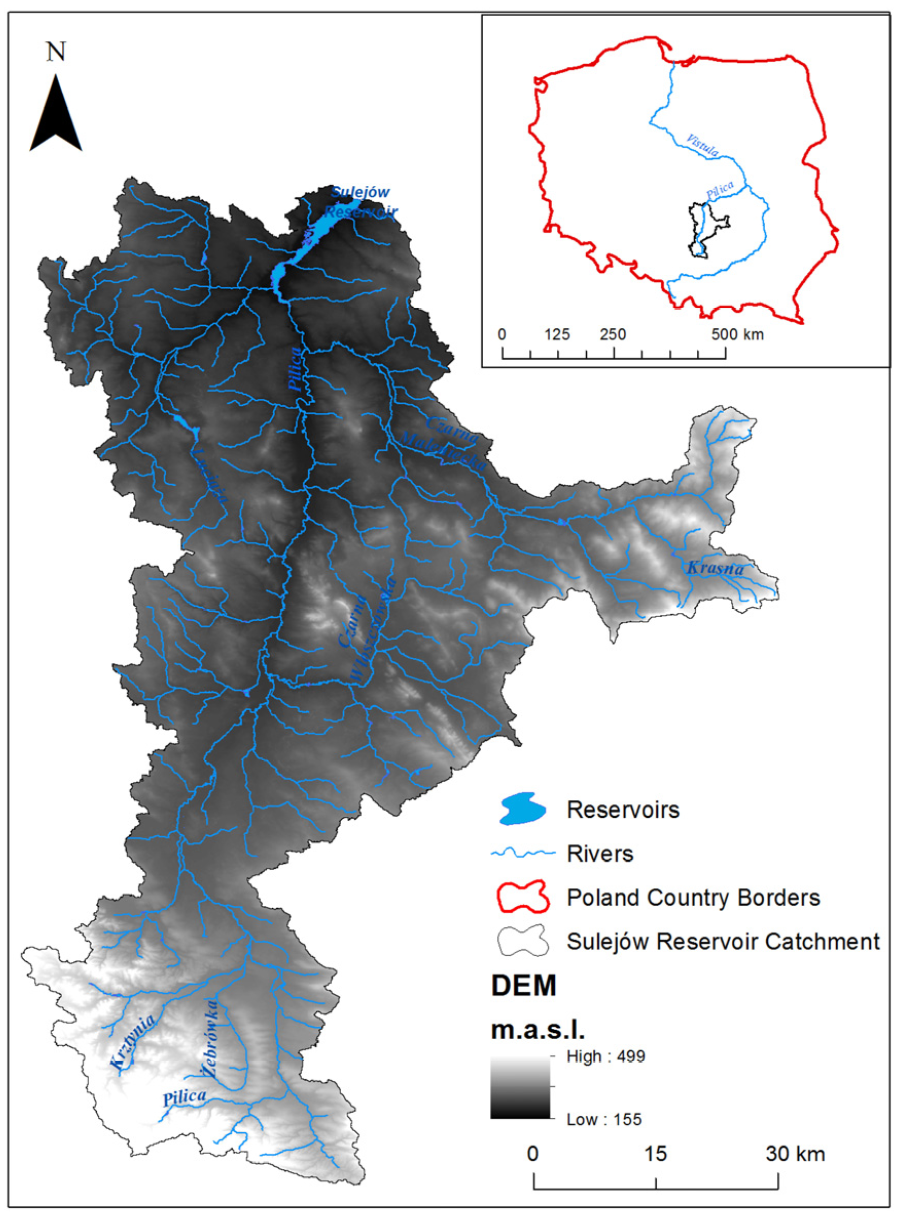
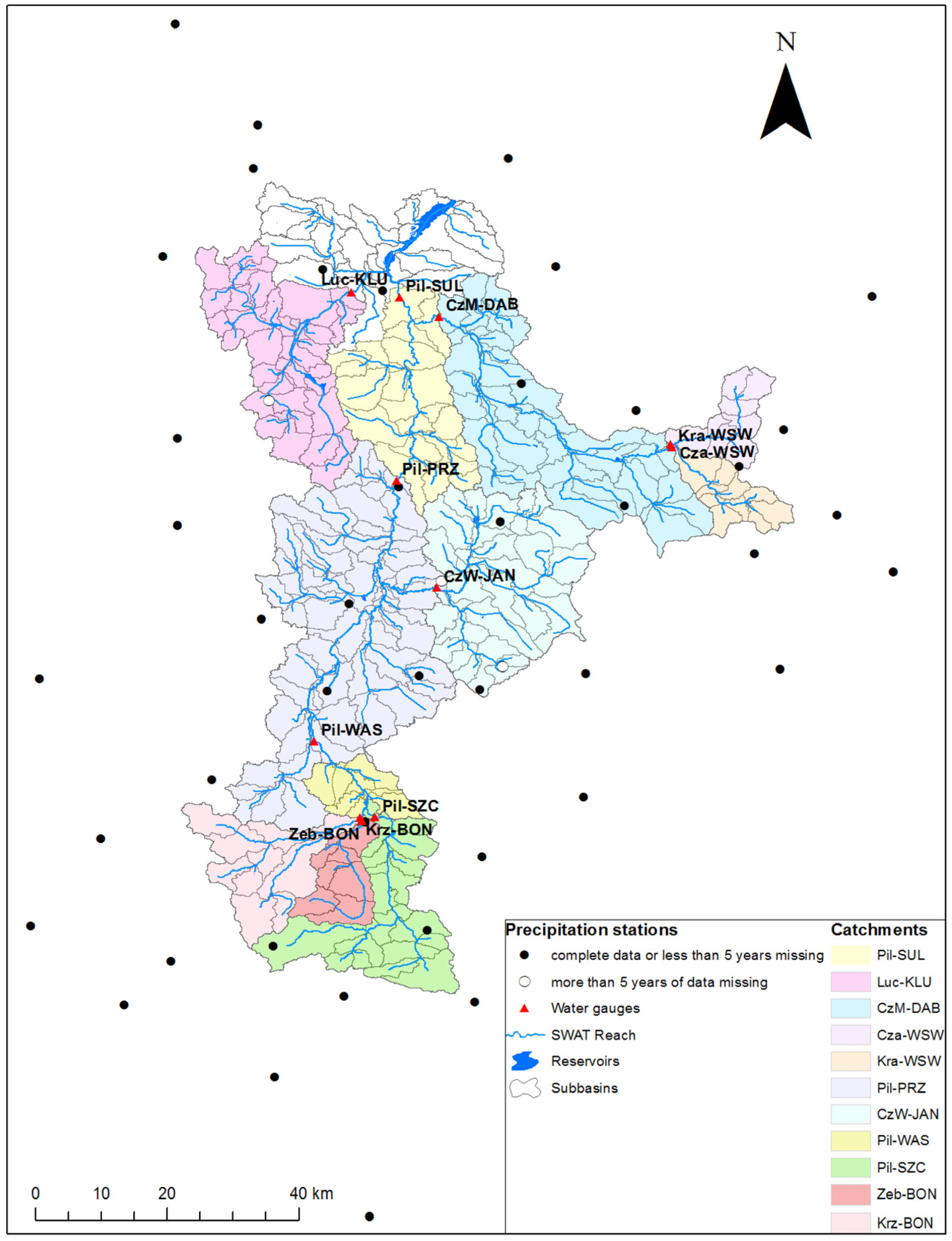
2.1. Study Area

2.2. SWAT Model
2.2.1. General Features
2.2.2. Model Setup
- -
- DEM based on the ASTER satellite data, 1:25,000 topographic map and Regional Water Management Authority (RZGW) water cadastre.
- -
- Land cover data derived from reclassified Corine Land Cover 2006 (CLC2006) available from General Directorate of Environmental Protection (GDOŚ).
- -
- Soil map composed of a 1:100,000 digital map from Institute of Soil Science and Plant Cultivation (IUNG) and 1:25,000 soil map available from Regional Directorate of State Forests (RDLP).
2.3. Precipitation Data and Interpolation Methods

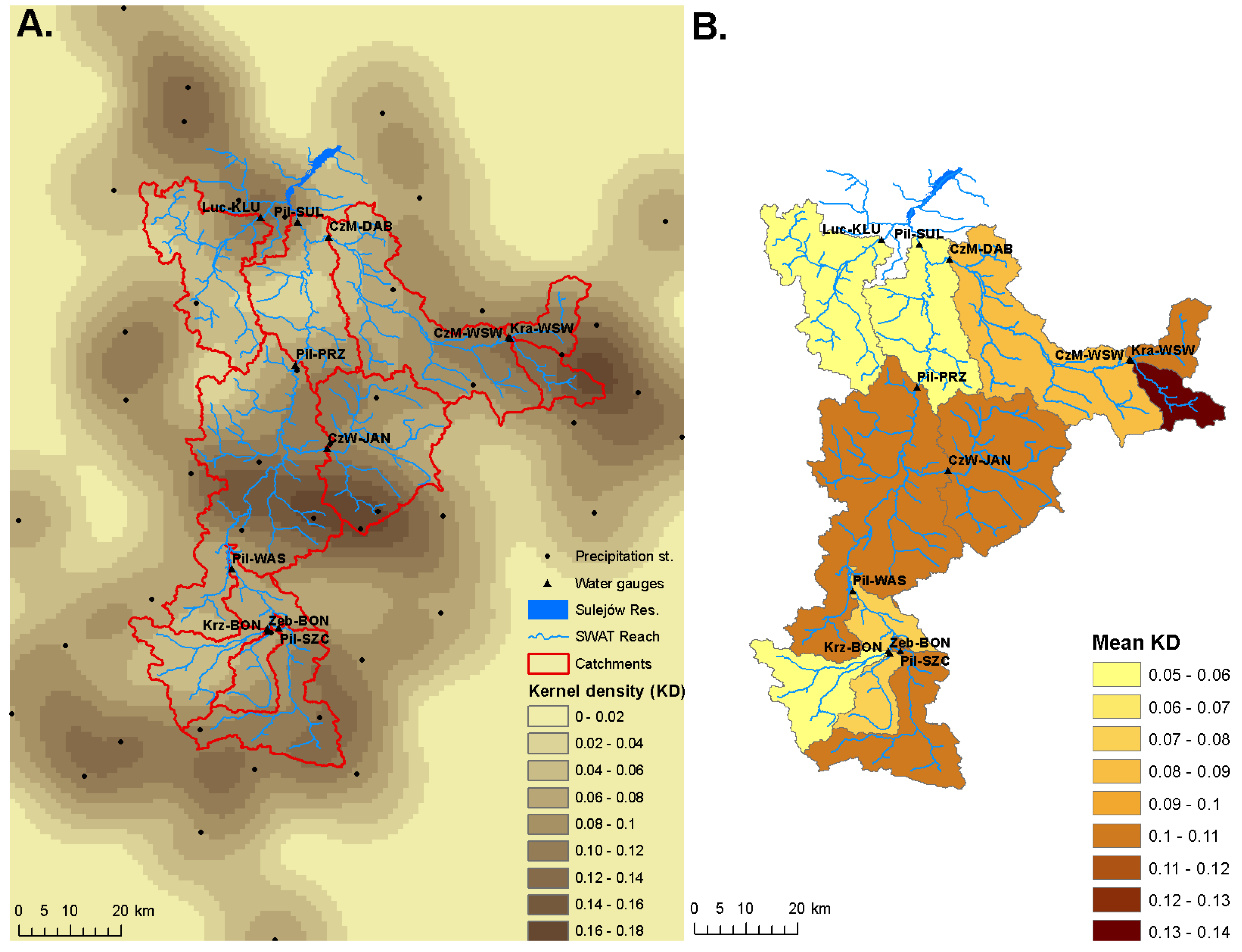
2.4. Precipitation Station Density Factor

2.5. Strategy for Evaluation of Hydrological Simulations
2.5.1. SWAT-CUP and SUFI-2

| Name | Lower Limit | Upper Limit | Definition |
|---|---|---|---|
| ESCO.hru 2 | 0.7 | 1 | Soil evaporation compensation factor |
| EPCO.hru 2 | 0 | 1 | Plant uptake compensation factor |
| SOL_Z().sol 1 | −0.4 | 0.4 | Depth from soil surface to the bottom of layer |
| SOL_AWC().sol 1 | −0.4 | 0.4 | Available water capacity of the soil layer |
| SOL_BD().sol 1 | −0.4 | 0.4 | Moist bulk density |
| SOL_K().sol 1 | −0.9 | 2 | Saturated hydraulic conductivity |
| HRU_SLP.hru 1 | −0.3 | 0.3 | Average slope steepness |
| ALPHA_BF.gw 2 | −0.9 | 2 | Baseflow alpha factor |
| GW_DELAY.gw 2 | 50 | 400 | Groundwater delay time |
| GWQMN.gw 2 | 0 | 1000 | Threshold depth of water in the shallow aquifer required for return flow to occur |
| GW_REVAP.gw 2 | 0.02 | 0.2 | Groundwater “revap” coefficient |
| RCHRG_DP.gw 2 | 0 | 0.3 | Deep aquifer percolation fraction |
| CN2.mgt 1 | −0.15 | 0.15 | Initial SCS (Soil Conservation Service) runoff curve nr for moisture condition II |
| SURLAG.bsn 2 | 0.3 | 3 | Surface runoff lag coefficient |
| SLSUBBSN.hru 1 | −0.3 | 0.3 | Average slope length (m) |
| CH_N2.rte 2 | 0.01 | 0.1 | Manning's “n” value for the main channel |
| CH_N1.sub 2 | 0.01 | 0.1 | Manning's “n” value for the tributary channel (-) |
| SMTMP.bsn 2 | −2 | 2 | Snow melt base temperature |
| TIMP.bsn 2 | 0 | 1 | Snow pack temperature lag factor |
| SNOCOVMX.bsn 2 | 0 | 40 | Minimum snow water content that corresponds to 100% snow cover |
2.5.2. The Observed Data and Catchment Properties
| No | Gauge Name | River Name | Code | A (km2) | Period of Available Data | Years | Flow (m3/s) | qm (m3/s/km2) | cv (-) | |
|---|---|---|---|---|---|---|---|---|---|---|
| Mean | St. Dev. | |||||||||
| 1 | Sulejów | Pilica | Pil-SUL | 3934 | 11/1/1983–10/31/2011 | 28 | 21.9 | 14.9 | 5.5 | 0.68 |
| 2 | Przedbórz | Pilica | Pil-PRZ | 2491 | 11/1/1983–10/31/2011 | 28 | 13.5 | 9.6 | 5.3 | 0.71 |
| 3 | Wąsosz | Pilica | Pil-WAS | 974 | 11/1/2005–10/31/2011 | 6 | 5.7 | 4.7 | 6.5 | 0.82 |
| 4 | Szczeko-ciny | Pilica | Pil-SZC | 360 | 11/1/1983–10/31/2009 | 26 | 1.8 | 1.3 | 5.0 | 0.69 |
| 5 | Kłudzice | Luciąża | Luc-KLU | 507 | 11/1/1983–10/31/2011 | 28 | 2.6 | 2.5 | 5.2 | 0.95 |
| 6 | Dąbrowa | Czarna Maleniecka | CzM-DAB | 946 | 11/1/1983–10/31/2008; 11/1/2009–10/21/2011 | 27 | 5.6 | 5.6 | 5.8 | 1.00 |
| 7 | Wąsosz-Stara Wieś | Czarna Maleniecka | Cza-WSW | 119 | 11/1/1991–10/31/2003 | 12 | 0.91 | 1.2 | 7.6 | 1.09 |
| 8 | Wąsosz-Stara Wieś | Krasna | Kra-WSW | 120 | 11/1/1991–10/31/2011 | 20 | 0.77 | 1.2 | 6.3 | 1.51 |
| 9 | Janusze-wice | Czarna Włoszczowska | CzW-JAN | 598 | 11/1/1983–10/31/2011 | 28 | 3.3 | 4.0 | 5.5 | 1.20 |
| 10 | Bonowice | Żebrówka | Zeb-BON | 128 | 11/1/1983–10/31/2009 | 26 | 0.51 | 0.47 | 6.5 | 0.82 |
| 11 | Bonowice | Krztynia | Krz-BON | 256 | 11/1/1990–10/31/2009 | 19 | 1.3 | 0.68 | 5.0 | 0.54 |
2.5.3. Study Design
3. Results and Discussion
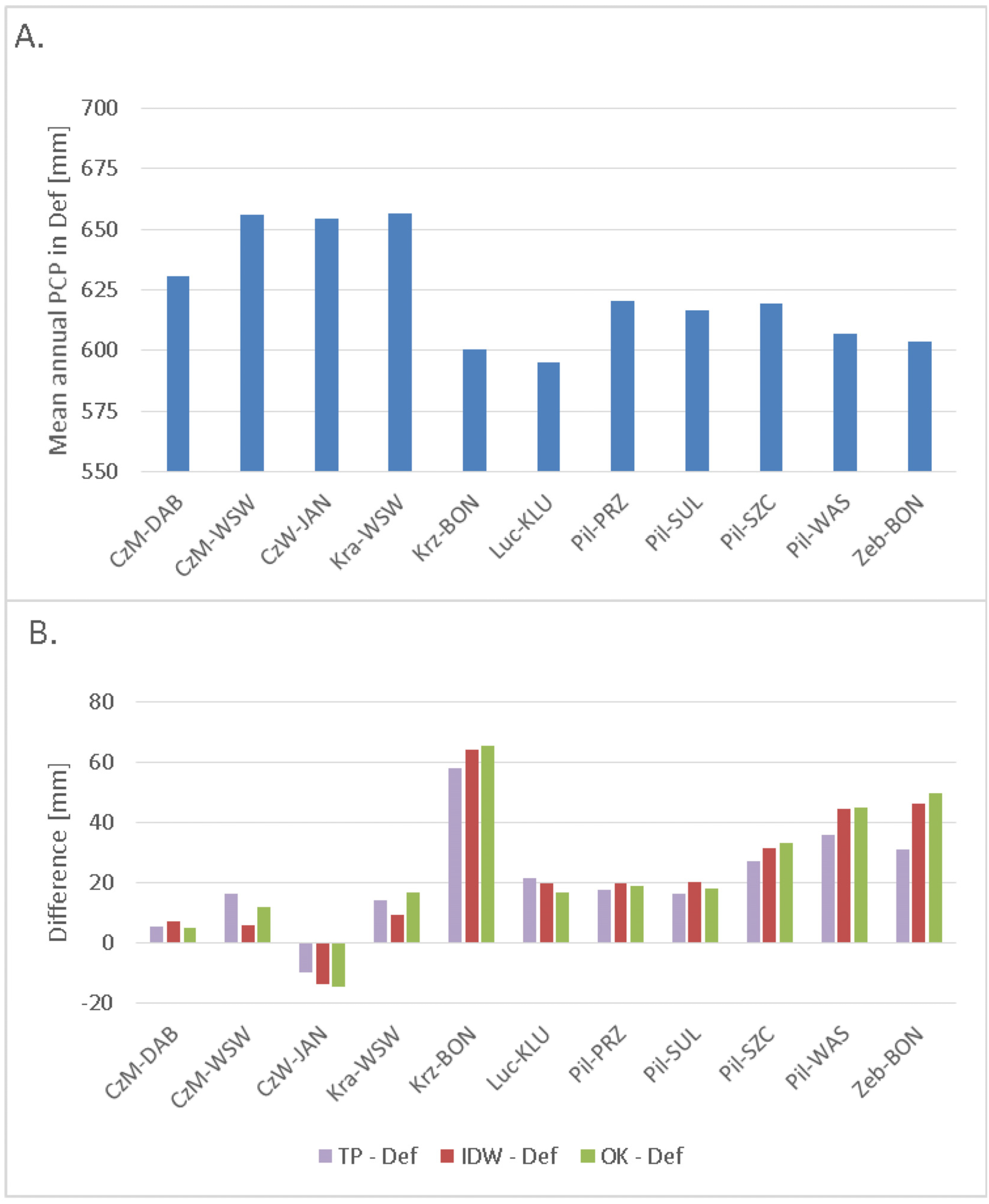
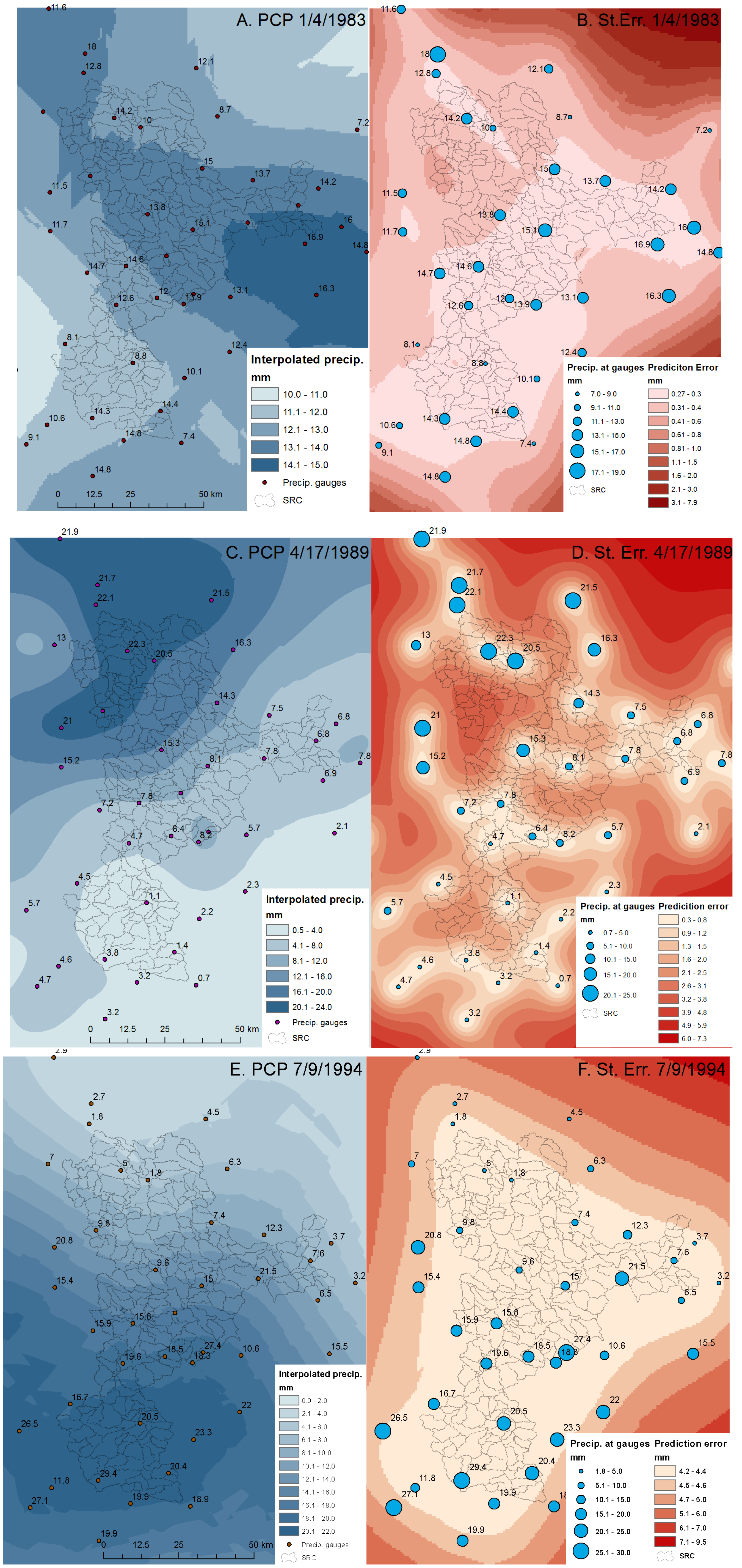
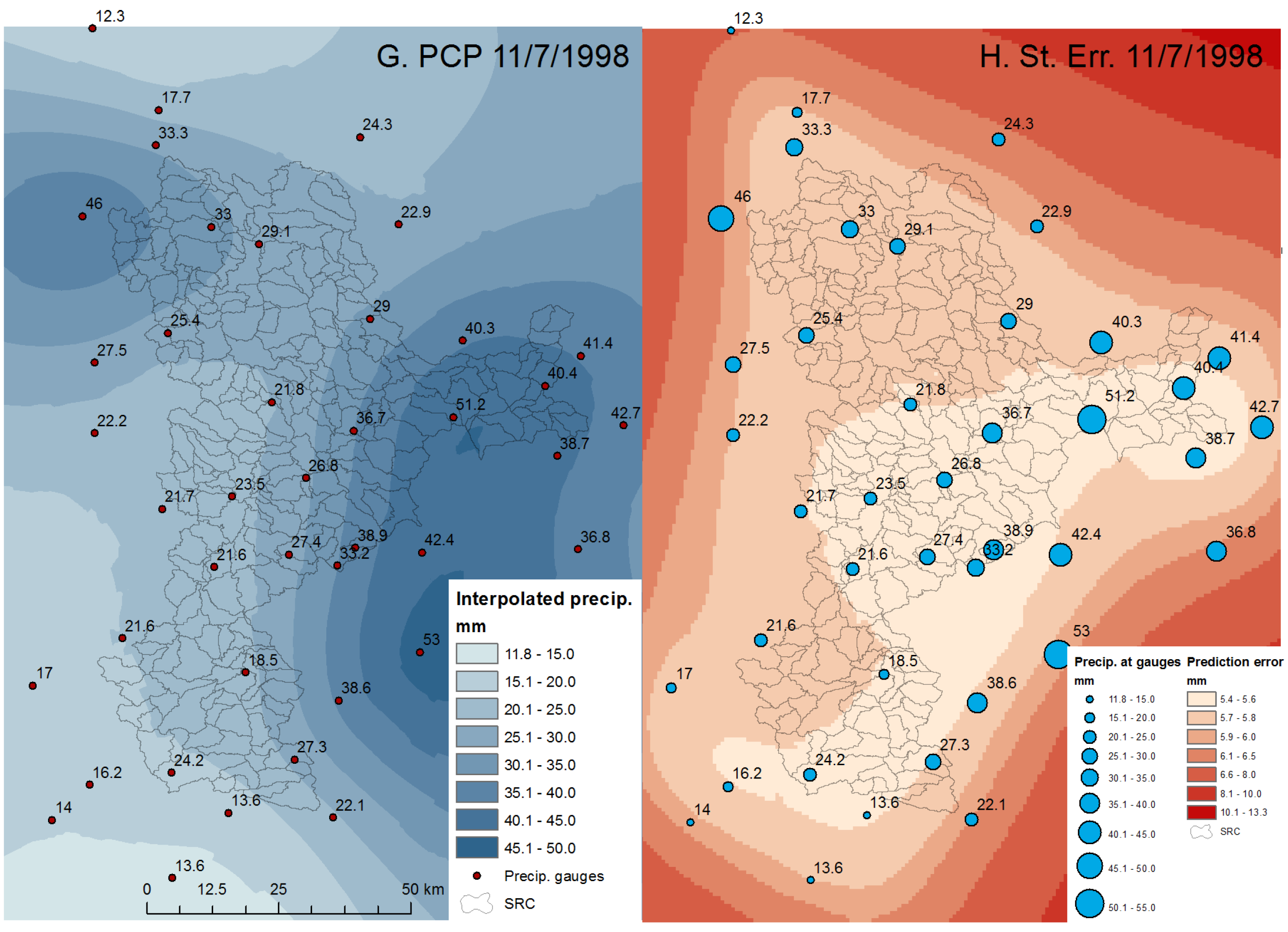
3.1. Evaluation of Interpolation Results


3.2. Effect of Interpolation Methods on Model Performance
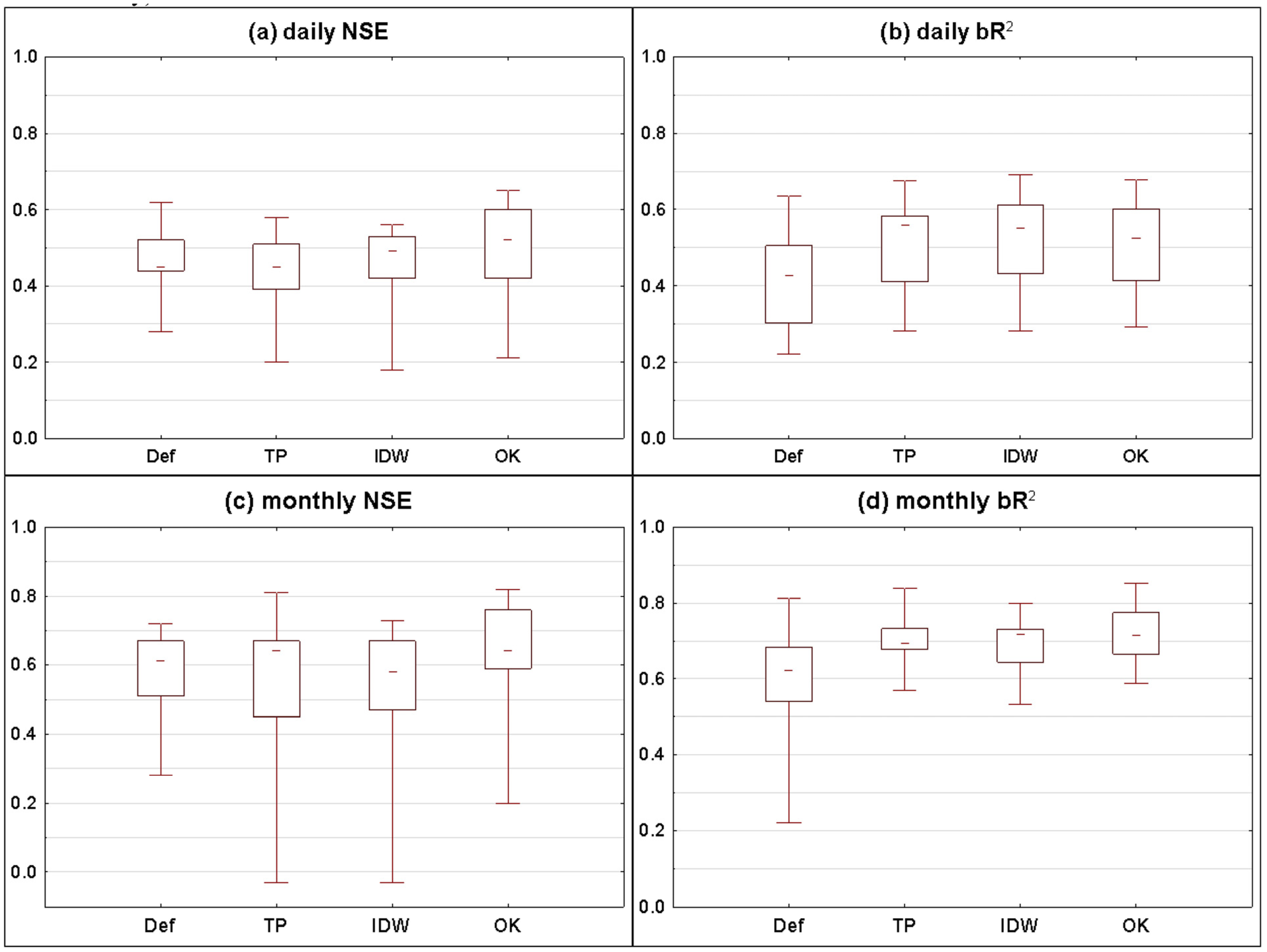
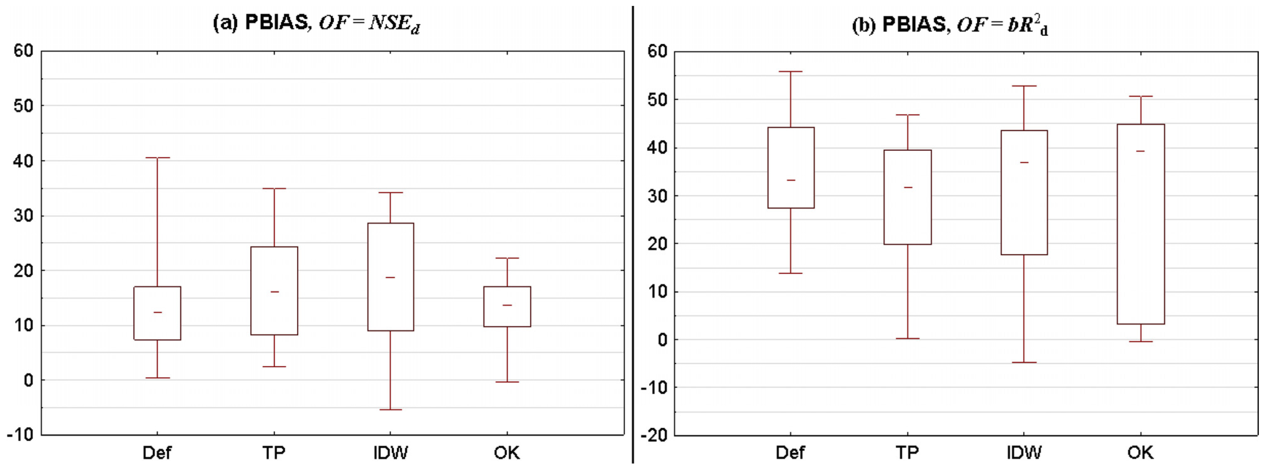
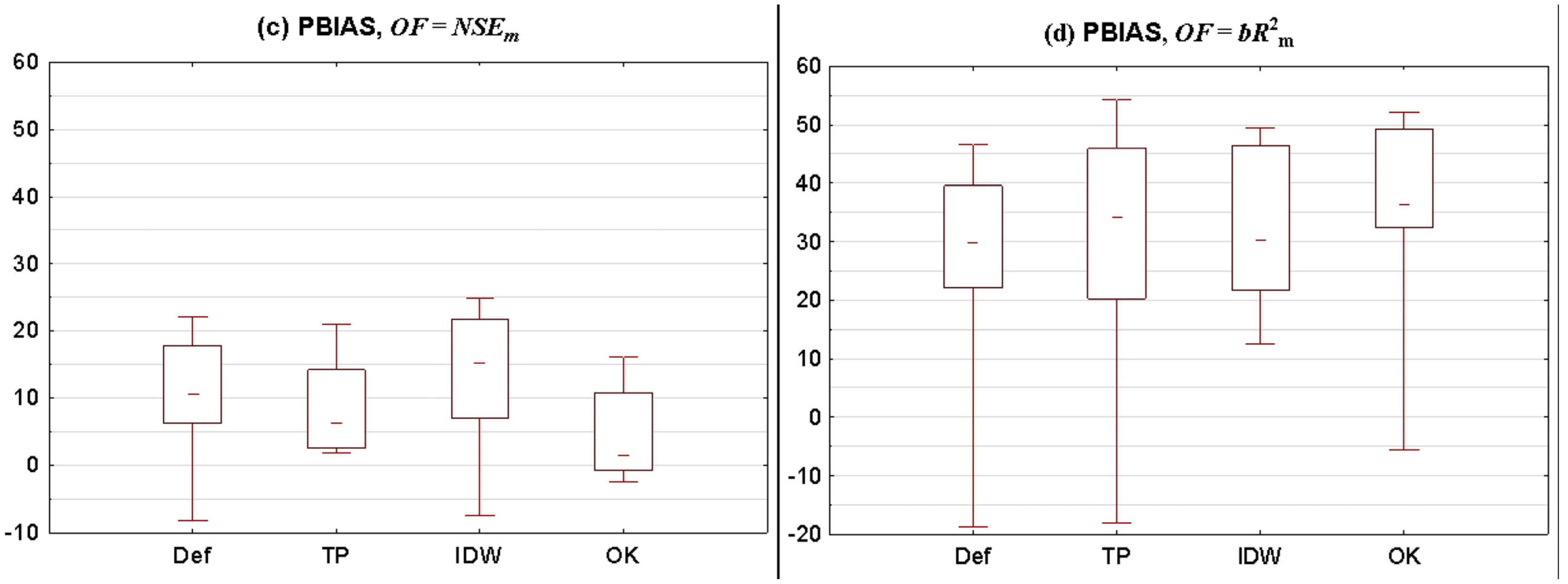
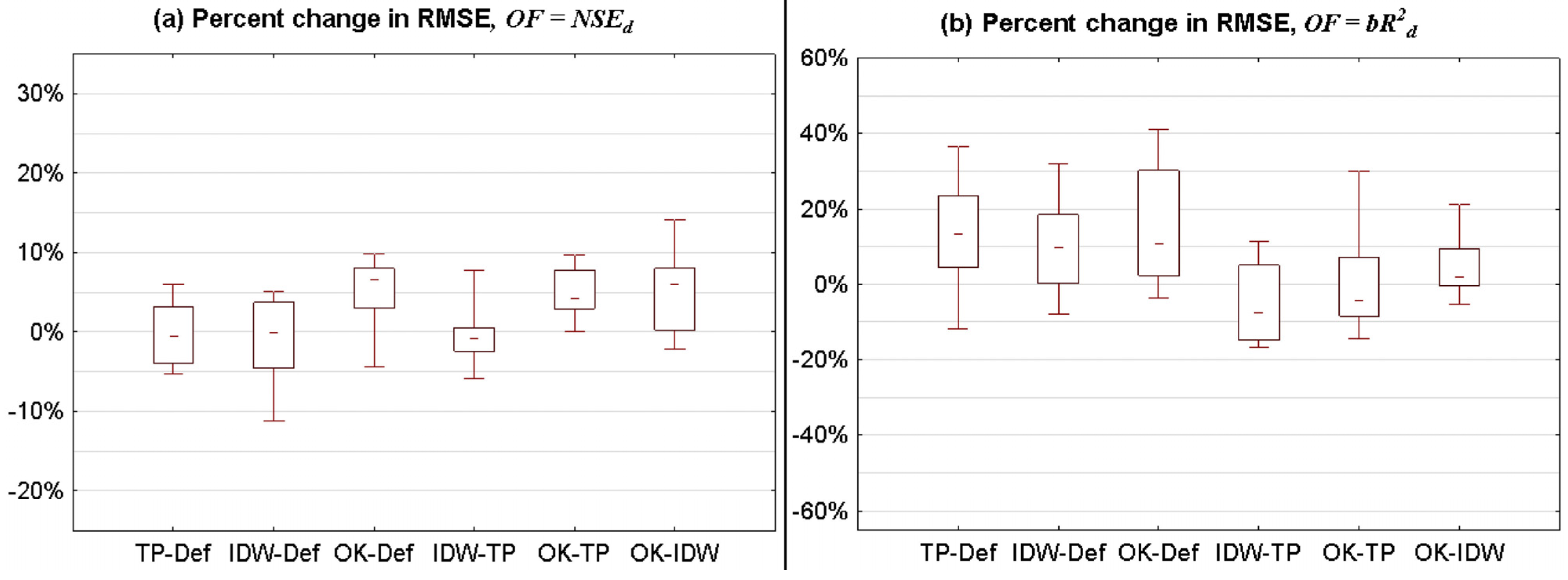
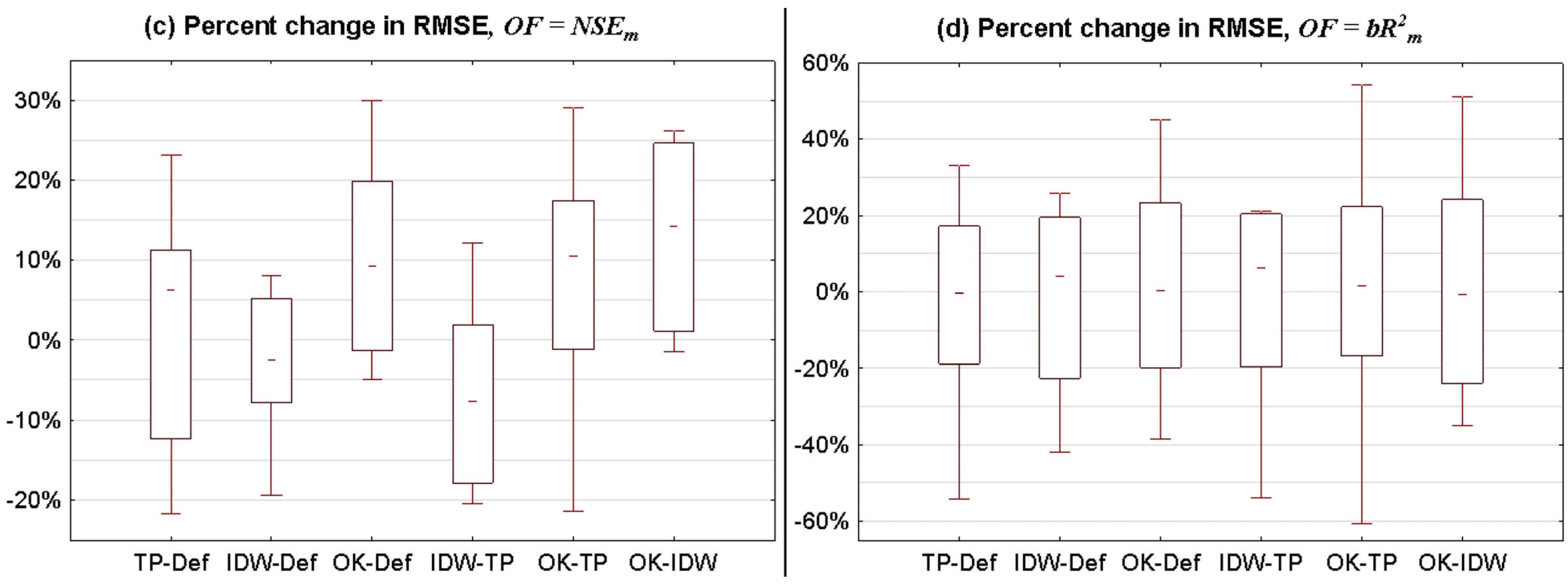
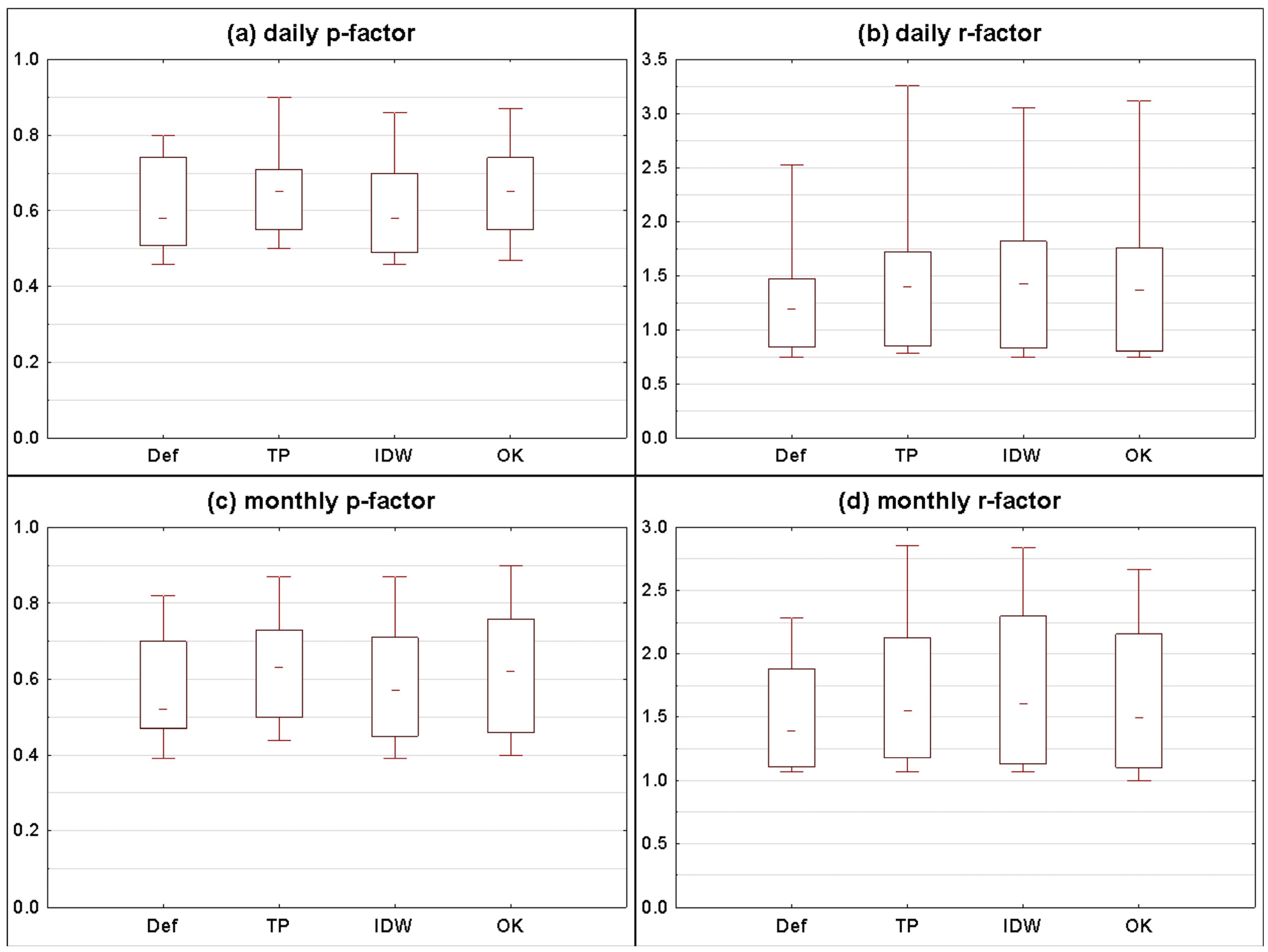
3.2.1. Statistical Summary for All Catchments


- (1)
- p-factor for method A is higher than p-factor for method B and r-factor for method A is not higher than r-factor for method B.
- (2)
- p-factor for method A is not lower than p-factor for method B and r-factor for method A is lower than r-factor for method B.

3.2.2. Relationship between the Objective Functions and Catchment Characteristics
| Catchment Properties | ||||||
|---|---|---|---|---|---|---|
| −0.15 | −0.36 | −0.14 | −0.36 | 0.00 | 0.28 | |
| −0.25 | −0.49 | 0.14 | −0.44 | 0.60 ‡ | 0.73 ‡ | |
| 0.19 | 0.28 | −0.10 | 0.18 | −0.46 | −0.44 | |
| 0.03 | 0.10 | −0.04 | 0.14 | 0.07 | −0.88 ‡ | |
| −0.54 † | −0.56 † | −0.60 † | −0.07 | −0.32 | 0.17 | |
| −0.13 | −0.13 | −0.16 | −0.09 | −0.22 | 0.08 | |
| −0.58 † | −0.60 ‡ | −0.59 † | 0.14 | −0.05 | 0.20 | |
| 0.81 ‡ | 0.78 ‡ | 0.79 ‡ | 0.19 | 0.51 | 0.24 | |
| 0.20 | −0.29 | −0.43 | −0.69 ‡ | −0.50 | −0.10 | |
| 0.27 | 0.03 | 0.35 | −0.40 | −0.04 | 0.34 | |
| 0.51 | 0.49 | −0.27 | −0.23 | −0.71 ‡ | −0.88 ‡ | |
| −0.60 † | −0.25 | 0.32 | 0.34 | 0.74 ‡ | −0.37 | |
| −0.54 † | −0.59 † | −0.70 ‡ | −0.52 † | −0.80 ‡ | −0.56 † | |
| −0.27 | −0.29 | −0.26 | −0.20 | −0.13 | −0.03 | |
| −0.25 | −0.16 | −0.33 | 0.26 | −0.38 | −0.55 † | |
| 0.63 ‡ | 0.53 † | 0.70 ‡ | 0.32 | 0.64 ‡ | 0.46 | |
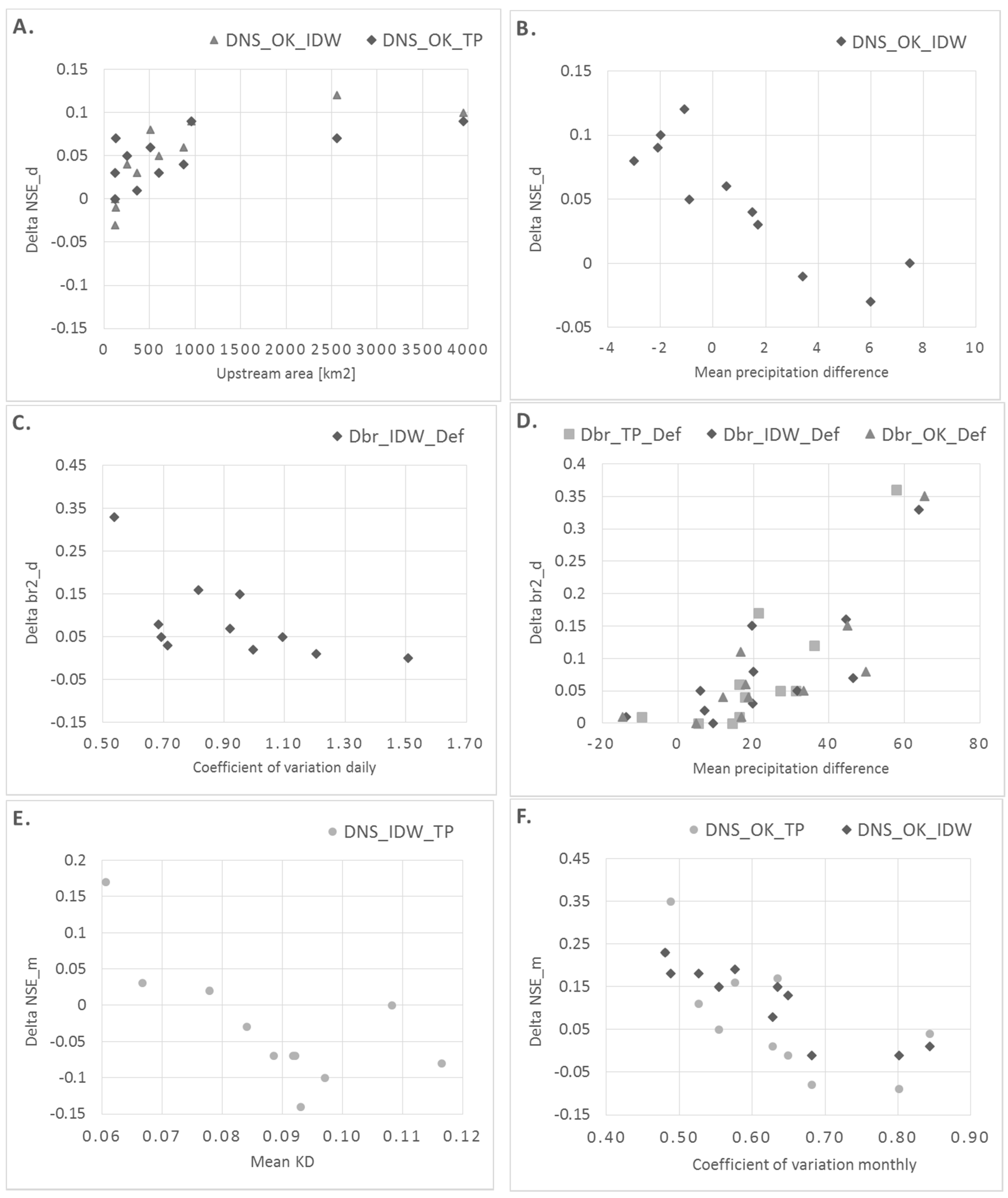
- (1)
- (Figure 10A,B): OK is superior over IDW and TP in catchments with larger drainage areas; OK is superior over IDW in catchments with small mean precipitation difference between these two methods.
- (2)
- (Figure 10C,D): IDW is superior over Def in catchments with lower daily (more stable flow regime); TP, IDW and OK are superior over Def in catchments with high positive difference in mean precipitation.
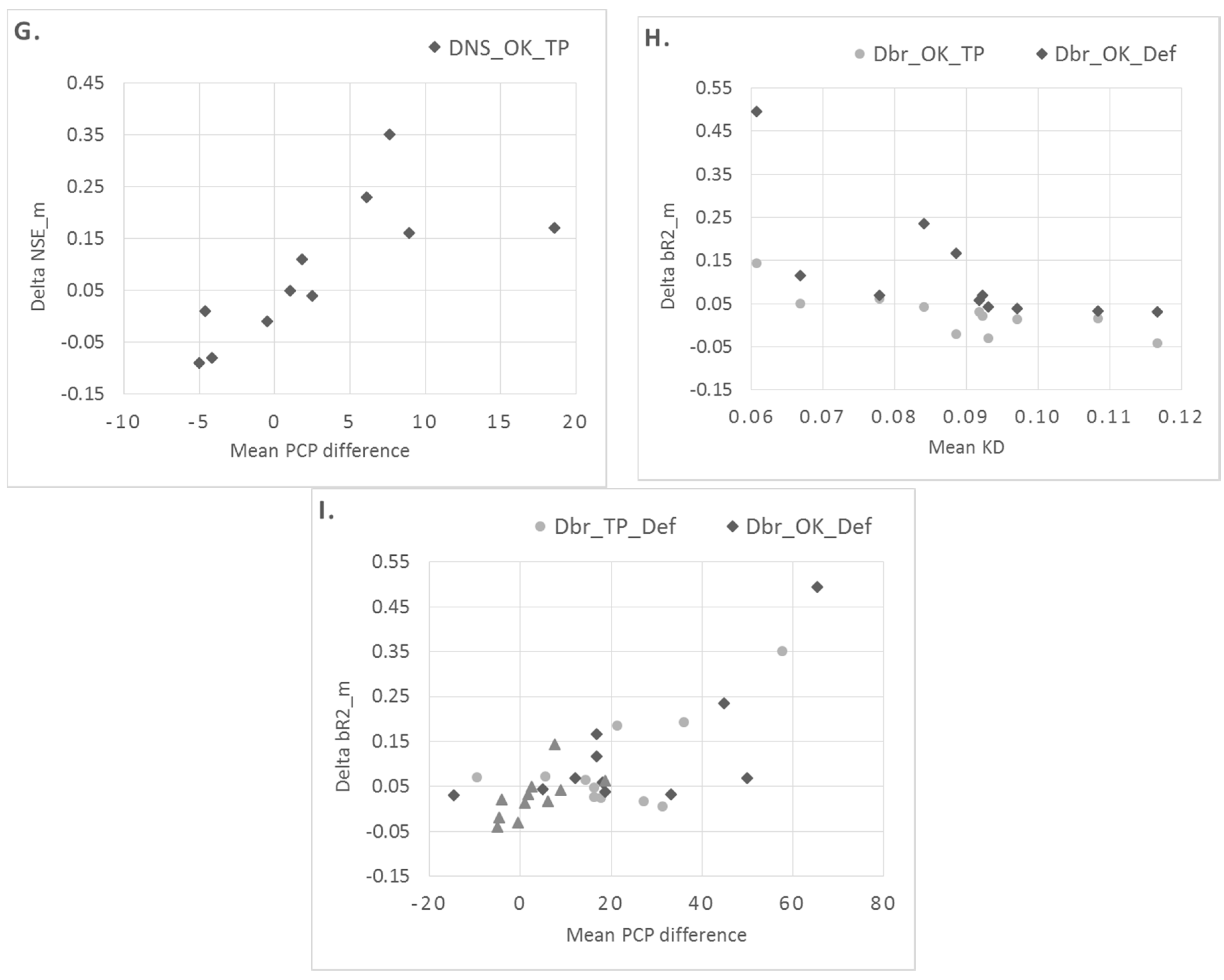
- (3)
- (Figure 10E–G): TP is superior over IDW in catchments with higher station densities; OK is superior over IDW and TP in catchments with lower monthly (more stable flow regime); OK is superior over TP in catchments for which the difference in mean precipitation between OK and TP is positive.
- (4)
- (Figure 10H,I): OK is superior over Def (more apparently) and TP (less apparently) in catchments with low station density. TP and OK are superior over Def in catchments with high positive difference in mean precipitation.


3.3. Discussion
| ID | Publication Code and Material | Catchment (Country) | Area (km2) | Number of Precipitation Gauges | Station Density (Stations/1000 km2) | Model Name | Simulation Period (Years) | Number of Flow Gauges | Analysis Time Step | Interpolation Methods | Evaluation Criterion | Main Conclusion |
|---|---|---|---|---|---|---|---|---|---|---|---|---|
| 1 | This paper; Figure 6 and Figure 8 | Pilica (PL) | 4,928 | 46 | 9.3 | SWAT | 30 | 11 | d, m | Def (NN), TP,IDW, OK | NSE, bR2 | OK, IDW, TP outperformed Def for bR2 for both daily and monthly time step; OK slightly better than others for NSE (daily and monthly) |
| 2 | Haberlandt1998 [22]; Figure 7A | Mackenzie (CA) | 1,800,000 | 81 | 0.05 | SLURP | 16 | 29 | m | NN, OK | Relative standard error | OK superior over NN but mainly in smaller subbasins (below 50,000 km2) |
| 3 | Hwang2012 [26]; Table 7, Figures 17 and 18 | Animas (CO, USA) | 1,792 | 37 | 20.6 | PRMS (distributed) | 26 | 1 | d, s, a | IDW, MLR, CMLR, LWP | RMSE, NSE, Flow statistics | All methods similar in terms of NSE and RMSE; all methods provide accurate timing of flood events but the magnitude is underestimated |
| 4 | Hwang2012 [26]; Tables 6 and 7, Figures 17 and 18 | Alapaha (GA, USA) | 3,626 | 28 | 7.7 | PRMS (distributed) | 22 | 1 | d, s, a | IDW, MLR, CMLR, LWP | RMSE, NSE, Flow statistics | LWP and MLR superior over CMLR in terms of NSE and RMSE; all methods provide accurate timing of flood events but the magnitude is underestimated |
| 5 | Masih2011 [23] Table 3, Figures 5–7 | Karkheh (IR) | 4,2620 | 41 | 0.96 | SWAT | 15 | 15 | d, m | Def (NN), IDEW | R2, NSE, Flow statistics | Little difference between two methods for R2, but IDEW superior over Def for NSE, especially in smaller subbasins (below 2500 km2) |
| 6 | Ruelland2008 [25]; Table 5, Figure 10 | Bani (ML, CI, BF) | 100,000 | 13 | 0.13 | Hydrostrahler | 6 | 7 | 10d | TP, IDW, Spline, OK | NSE, VE, PE | The best results in terms of selected criteria were obtained for IDW, intermediate for TP and OK and the worst for Spline; all methods underestimated flood peaks |
| 7 | Shen2013 [27]; Tables 2 and 3, Figure 3a,b | Daning (CN) | 4,426 | 19 | 4.3 | SWAT | 7 | 3 | m | Def (NN), TP, IDW, Dis-Kriging, CoKriging | NSE, flow statistics | All methods showed an improvement over the Default method in terms of NSE (the highest for CoKriging); all methods underestimate most of flow characteristics |
| 8 | Wagner2012 [28]; Tables 4 and 5, Figure 8 | Mula and Mutha (IN) | 2,036 | 16 | 7.9 | SWAT | 21 | 4 | d | RIDWx, RIDWtrmm, RKx, RKtrmm | NSE, PBIAS, flow statistics | RIDWTrmm and RKTrmm outperform RIDWX and RKX in terms of NSE and PBIAS; RKX overestimates runoff and does not reproduce right timing of floods in contrast to RKTrmm |
4. Conclusions
Acknowledgments
Author Contributions
Conflicts of Interest
References
- Arnold, J.G.; Srinivasan, R.; Muttiah, R.S.; Williams, J.R. Large area hydrologic modeling and assessment—Part 1: Model development. J. Am. Water Resour. Assoc. 1998, 34, 73–89. [Google Scholar] [CrossRef]
- Gassman, P.W. Worldwide use of SWAT: 2012 update. In Proceedings of the 2012 International SWAT Conference, India Habitat Centre, Lodhi Road, New Delhi, India, 18–20 July 2012.
- Smith, M.B.; Korena, V.I.; Zhanga, Z.; Reeda, S.M.; Panb, J.J.; Moreda, F. Runoff response to spatial variability in precipitation: an analysis of observed data. J. Hydrol. 2004, 298, 267–286. [Google Scholar] [CrossRef]
- Tetzlaff, D.; Uhlenbrook, S. Significance of spatial variability in precipitation for process-oriented modelling: Results from two nested catchments using radar and ground station data. Hydrol. Earth Syst. Sci. 2005, 9, 29–41. [Google Scholar] [CrossRef]
- Price, K.; Purucker, S.T.; Kraemer, S.R.; Babendreier, J.E.; Knightes, C.D. Comparison of radar and gauge precipitation data in watershed models across varying spatial and temporal scales. Hydrol. Process. 2014, 28, 3505–3520. [Google Scholar] [CrossRef]
- Caracciolo, D.; Arnone, E.; Noto, L. Influence of Spatial Precipitation Sampling on Hydrological Response at the Catchment Scale. J. Hydrol. Eng. 2014, 19, 544–553. [Google Scholar] [CrossRef] [Green Version]
- Chintalapudi, S.; Sharif, H.O.; Xie, H. Sensitivity of Distributed Hydrologic Simulations to Ground and Satellite Based Rainfall Products. Water 2014, 6, 1221–1245. [Google Scholar] [CrossRef]
- Di Piazza, A.; Lo Conti, F.; Noto, L.V.; la Loggia, G. Comparative analysis of different techniques for spatial interpolation of rainfall data to create a serially complete monthly time series of precipitation for Sicily, Italy. Int. J. Appl. Earth Obs. Geoinf. 2011, 13, 396–408. [Google Scholar]
- Yang, D.; Goodison, B.E.; Metcalfe, J.R.; Louie, P.; Leavesley, G.; Emerson, D.; Hanson, C.L.; Golubev, V.S.; Elomaa, E.; Gunther, T.; et al. Quantification of precipitation measurement discontinuity induced by wind shields on national gauges. Water Resour. Res. 1999, 35, 491–508. [Google Scholar] [CrossRef]
- Mishra, A.K. Effect of rain gauge density over the accuracy of rainfall: A case study over Bangalore, India. SpringerPlus 2013, 2, 1–7. [Google Scholar] [CrossRef] [PubMed]
- Majewski, W. Urban flash flood in Gdańsk, 2001. Ann. Wars. Univ. Life Sci. SGGW Land Reclam. 2008, 39, 129–137. [Google Scholar]
- Weedon, G.P.; Gomes, S.; Viterbo, P.; Shuttleworth, W.J.; Blyth, E.; Österle, H.; Adam, J.C.; Bellouin, N.; Boucher, O.; Best, M. Creation of the WATCH Forcing data and its use to assess global and regional reference crop evaporation over land during the twentieth century. J. Hydrometerol. 2011, 12, 823–848. [Google Scholar] [CrossRef]
- Kalin, L.; Hantush, M. Hydrologic Modeling of an Eastern Pennsylvania Watershed with NEXRAD and Rain Gauge Data. J. Hydrol. Eng. 2006, 11, 555–569. [Google Scholar] [CrossRef]
- Sun, X.; Mein, R.G.; Keenan, T.D.; Elliott, J.F. Flood estimation using radar and raingauge data. J. Hydrol. 2000, 239, 4–18. [Google Scholar] [CrossRef]
- Sharma, S.; Isik, S.; Srivastava, P.; Kalin, L. Deriving spatially distributed precipitation data using the artificial neural network and multilinear regression models. J. Hydrol. Eng. 2012, 18, 194–205. [Google Scholar] [CrossRef]
- Morin, E.; Krajewski, W.F.; Goodrich, D.C.; Gao, X.; Sorooshian, S. Estimating Rainfall Intensities from Weather Radar Data: The Scale-Dependency Problem. J. Hydrometeor. 2003, 4, 782–797. [Google Scholar] [CrossRef]
- Ly, S.; Charles, C.; Degré, A. Different methods for spatial interpolation of rainfall data for operational hydrology and hydrological modeling at watershed scale. A review. Biotechnol. Agron. Soc. Environ. 2013, 17, 392–406. [Google Scholar]
- Hartkamp, A.D.; de Beurs, K.; Stein, A.; White, J.W. Interpolation Techniques for Climate Variables; CIMMYT: Mexico D.F., Mexico, 1999. [Google Scholar]
- Goovaerts, P. Geostatistical approaches for incorporating elevation into the spatial interpolation of rainfall. J. Hydrol. 2000, 228, 113–129. [Google Scholar] [CrossRef]
- Zhang, X.; Srinivasan, R. GIS-based spatial precipitation estimation: A comparison of geostatistical approaches. J. Am. Water Resour. Assoc. 2009, 45, 894–906. [Google Scholar] [CrossRef]
- Tabios, G.Q.; Salas, J.D. A comparative analysis of techniques for spatial interpolation of precipitation. Water Resour. Bull. 1985, 21, 365–380. [Google Scholar] [CrossRef]
- Haberlandt, U.; Kite, G.W. Estimation of daily space-time precipitation series for macroscale hydrological modelling. Hydrol. Process. 1998, 12, 1419–1432. [Google Scholar] [CrossRef]
- Masih, I.; Maskey, S.; Uhlenbrook, S.; Smakhtin, V. Assessing the Impact of Areal Precipitation Input on Streamflow Simulations Using the SWAT Model. J. Am. Water Resour. Assoc. 2011, 47, 179–195. [Google Scholar] [CrossRef]
- Blöschl, G. Scale and scaling in hydrology. In Wiener Mitteilungen, Wasser–Abwasser–Gewässer; Technical University of Vienna: Vienna, Austria, 1996. [Google Scholar]
- Ruelland, D.; Ardoin-Bardin, S.; Billen, G.; Servat, E. Sensitivity of a lumped and semi-distributed hydrological model to several methods of rainfall interpolation on a large basin in West Africa. J. Hydrol. 2008, 361, 96–117. [Google Scholar] [CrossRef]
- Hwang, Y.; Clark, M.; Rajagopalan, B.; Leavesley, G. Spatial interpolation schemes of daily precipitation for hydrologic modeling. Stoch. Environ. Res. Risk Assess. 2012, 26, 295–320. [Google Scholar] [CrossRef]
- Shen, Z.; Chen, L.; Liao, Q.; Liu, R.; Hong, Q. Impact of spatial rainfall variability on hydrology and nonpoint source pollution modeling. J. Hydrol. 2012, 472, 205–215. [Google Scholar] [CrossRef]
- Wagner, P.D.; Fiener, P.; Wilken, F.; Kumar, S.; Schneider, K. Comparison and evaluation of spatial interpolation schemes for daily rainfall in data scarce regions. J. Hydrol. 2012, 465, 388–400. [Google Scholar] [CrossRef]
- Boer, E.P.J.; de Beurs, K.M.; Hartkamp, A.D. Kriging and thin plate splines for mapping climate Variables. Int. J. Appl. Earth Obs. Geoinf. 2001, 3, 146–154. [Google Scholar] [CrossRef]
- Todini, E.; Pellegrini, F.; Mazzetti, C. Influence of parameter estimation uncertainty in Kriging: Part 2. Test and case study applications. Hydrol. Earth Syst. Sci. 2001, 5, 225–232. [Google Scholar] [CrossRef]
- Marqunez, J.; Lastra, J.; Garcia, P. Estimation models for precipitation in mountainous regions: the use of GIS and multivariate analysis. J. Hydrol. 2003, 270, 1–11. [Google Scholar] [CrossRef]
- Vicent-Serrano, S.M.; Saz-Sanchez, M.A.; Cuadrat, J.M. Comparative analysis of interpolation methods in the middle Ebro Valley (Spain): Application to annual precipitation and temperature. Clim. Res. 2003, 24, 161–180. [Google Scholar] [CrossRef]
- Lloyd, C.D. Assessing the effect of integrating elevation data into the estimation of monthly precipitation in Great Britain. J. Hydrol. 2005, 308, 128–150. [Google Scholar] [CrossRef]
- Vaze, J.; Post, D.A.; Chiew, F.H.S.; Perraud, J.M.; Viney, N.R.; Teng, J. Climate non-stationarity—Validity of calibrated rainfall–runoff models for use in climate change studies. J. Hydrol. 2010, 394, 447–457. [Google Scholar] [CrossRef]
- Hattermann, F.F.; Wattenbach, M.; Krysanova, V.; Wechsung, F. Runoff simulations on the macroscale with the ecohydrological model SWIM in the Elbe catchment–validation and uncertainty analysis. Hydrol. Process. 2005, 19, 693–714. [Google Scholar] [CrossRef]
- Wagner, I.; Zalewski, M. Effect of hydrological patterns of tributaries on biotic processes in a lowland reservoir—Consequences for restoration. Ecol. Eng. 2000, 16, 79–90. [Google Scholar] [CrossRef]
- Neitsch, S.; Arnold, J.; Kiniry, J.; Williams, J. Soil and Water Assessment Tool Theoretical Documentation Version 2009; Texas Water Resources Institute Technical Report No. 406; Texas A & M University: Temple, TX, USA, 2011. [Google Scholar]
- Arnold, J.; Kiniry, J.; Srinivasan, R.; Williams, J.; Haney, E.; Neitsch, S. Soil and Water Assessment Tool Input/Output File Documentation Version 2009; Texas Water Resources Institute Technical Report No. 365; Texas A & M University: Temple, TX, USA, 2011. [Google Scholar]
- Winchell, M.; Srinivasan, R.; Luzio, M.D.; Arnold, J. ArcSWAT Interface for SWAT2009. User’s Guide; Technical Report; Blackland Research and Extension Center; Grassland, Soil and Water Research Laboratory ,Texas A & M University: Temple, TX, USA, 2010. [Google Scholar]
- Sharpley, A.N.; Williams, J.R. Erosion/Productivity Impact Calculator, 1. Model Documentation; USDA-ARS Technical Bulletin Vol. 1768; Department of Agriculture: Washington, DC, USA, 1990; pp. 3–9. [Google Scholar]
- Thiessen, A.H. Precipitation averages for large areas. Monthly Weather Rev. 1911, 39, 1082–1084. [Google Scholar] [CrossRef]
- Meijerink, A.M.J.; de Brouwer, H.A.M.; Mannaerts, C.M.; Valenzuela, C.R. Introduction to Use of Geographic Information Systems for Practical Hydrology; International Institute for Aerospace Survey and Earth Sciences: Enschede, The Netherlands, 1994. [Google Scholar]
- Isaaks, E.H.; Srivastava, R.M. Applied Geostatistics; Oxford University Press: New York, NY, USA, 1998. [Google Scholar]
- Ly, S.; Charles, C.; Degre, A. Geostatistical interpolation of daily rainfall at catchment scale: The use of several variogram models in the Ourthe and Ambleve catchments, Belgium. Hydrol. Earth Syst. Sci. 2011, 15, 2259–2274. [Google Scholar] [CrossRef]
- Larson, L.L.; Peck, E.L. Accuracy of precipitation measurements for hydrologic modeling. Water Resour. Res. 1974, 10, 857–863. [Google Scholar] [CrossRef]
- ArcGIS Desktop 10 Help. Available online: http://help.arcgis.com/en/arcgisdesktop/10.0/help/index.html#//0031000000m3000000 (accessed on 9 February 2015).
- Silverman, B.W. Density Estimation for Statistics and Data Analysis; Chapman and Hall: New York, NY, USA, 1986. [Google Scholar]
- Piniewski, M.; Kardel, I.; Giełczewski, M.; Marcinkowski, P.; Okruszko, T. Climate change and agricultural development: Adapting Polish agriculture to reduce future nutrient loads in a coastal watershed. Ambio 2014, 43, 644–660. [Google Scholar] [CrossRef] [PubMed]
- Abbaspour, K. SWAT-CUP2: SWAT Calibration and Uncertainty Programs—A User Manual; Department of Systems Analysis, Integrated Assessment and Modelling(SIAM), Eawag, Swiss Federal Institute of Aquatic Science and Technology: Duebendorf, Switzerland, 2009. [Google Scholar]
- Abbaspour, K.; Johnson, C.A.; van Genuchten, M.T. Estimating Uncertain Flow and Transport Parameters Using a Sequential Uncertainty Fitting Procedure. Vadose Zone J. 2004, 3, 1340–1352. [Google Scholar] [CrossRef]
- Piniewski, M.; Okruszko, T. Multi-site calibration and validation of the hydrological component of SWAT in a large lowland catchment. In Modelling of Hydrological Processes in the Narew Catchment; Świątek, D., Okruszko, T., Eds.; Springer: Berlin, Germany, 2011; pp. 15–41. [Google Scholar]
- Moriasi, D.N.; Arnold, J.G.; van Liew, M.W.; Bingner, R.L.; Harmel, R.D.; Veith, T.L. Model evaluation guidelines for systematic quantification of accuracy in watershed simulations. Tran. ASABE 2007, 50, 885–900. [Google Scholar] [CrossRef]
- Gupta, H.V.; Sorooshian, S.; Yapo, P.O. Status of automatic calibration for hydrologic models: Comparison with multilevel expert calibration. J. Hydrol. Eng. 1999, 4, 135–143. [Google Scholar] [CrossRef]
- Randles, R.H. Wilcoxon signed rank test. Encycl. Stat. Sci. 1988, 9, 613–616. [Google Scholar]
- Tobin, C.; Nicotina, L.; Parlange, M.B.; Berne, A.; Rinaldo, A. Improved interpolation of meteorological forcings for hydrologic applications in a Swiss Alpine region. J. Hydrol. 2011, 401, 77–89. [Google Scholar] [CrossRef]
- Zhu, Q.; Zhang, X.; Ma, C.; Gao, X.; Xu, Y. Investigating the uncertainty and transferability of parameters in SWAT model under climate change. Hydrol. Sci. J. 2014, in press. [Google Scholar]
- Heistermann, M.; Kneis, D. Benchmarking quantitative precipitation estimation by conceptual rainfall-runoff modeling. Water Resour. Res. 2011, 47. [Google Scholar] [CrossRef]
- Yapo, P.O.; Gupta, H.V.; Sorooshian, S. Multi-objective global optimization for hydrologic models. J. Hydrol. 1998, 204, 83–97. [Google Scholar] [CrossRef]
© 2015 by the authors; licensee MDPI, Basel, Switzerland. This article is an open access article distributed under the terms and conditions of the Creative Commons Attribution license (http://creativecommons.org/licenses/by/4.0/).
Share and Cite
Szcześniak, M.; Piniewski, M. Improvement of Hydrological Simulations by Applying Daily Precipitation Interpolation Schemes in Meso-Scale Catchments. Water 2015, 7, 747-779. https://doi.org/10.3390/w7020747
Szcześniak M, Piniewski M. Improvement of Hydrological Simulations by Applying Daily Precipitation Interpolation Schemes in Meso-Scale Catchments. Water. 2015; 7(2):747-779. https://doi.org/10.3390/w7020747
Chicago/Turabian StyleSzcześniak, Mateusz, and Mikołaj Piniewski. 2015. "Improvement of Hydrological Simulations by Applying Daily Precipitation Interpolation Schemes in Meso-Scale Catchments" Water 7, no. 2: 747-779. https://doi.org/10.3390/w7020747