
Application of the Multimodel Ensemble Kalman Filter Method in Groundwater System


Abstract
:1. Introduction
2. Methodology
2.1. Theoretical Background
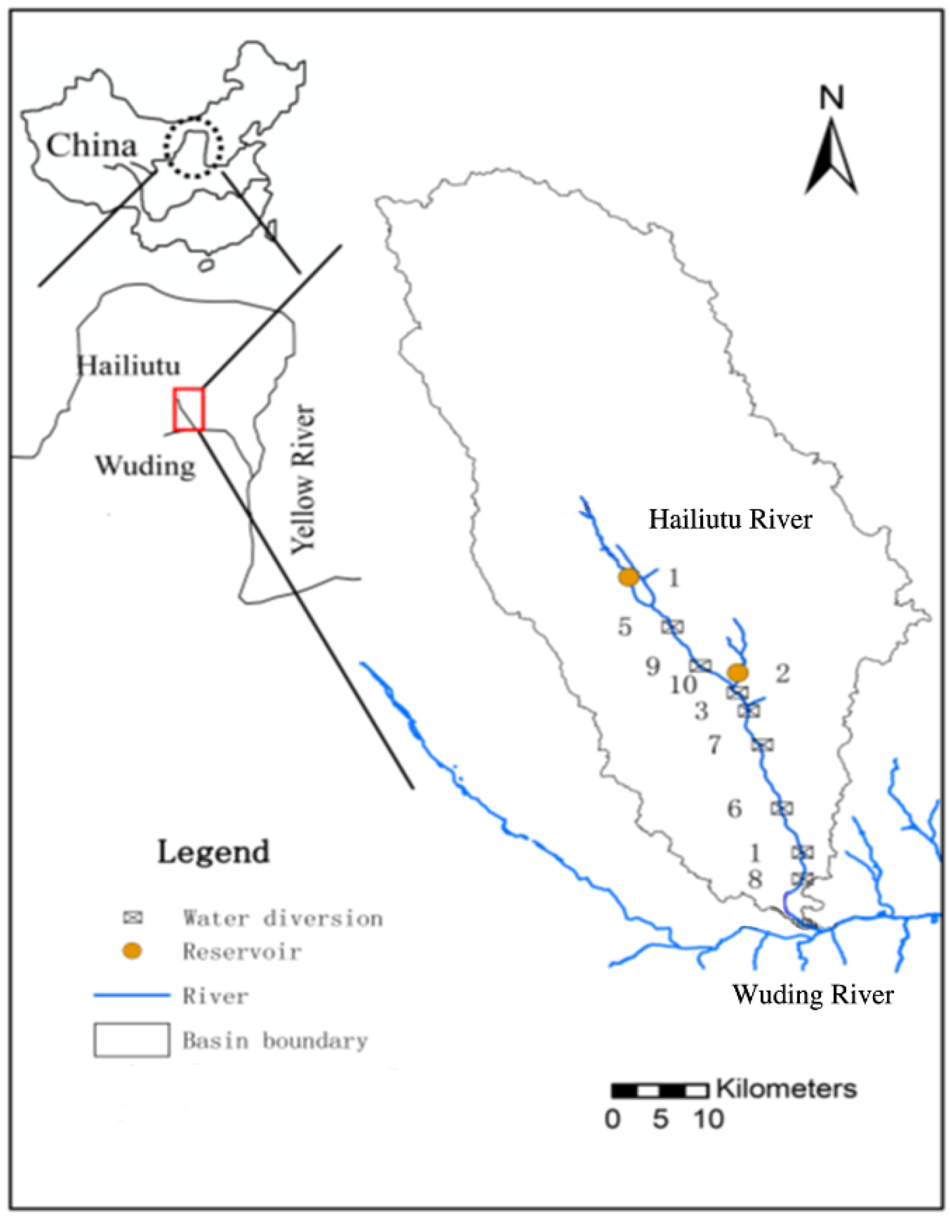
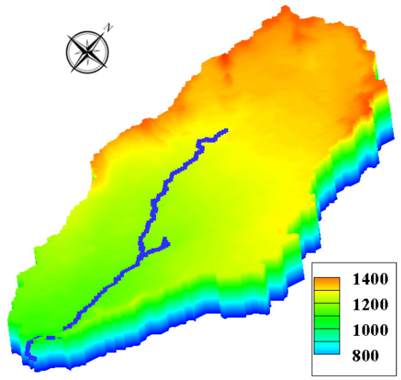
2.2. Study Area


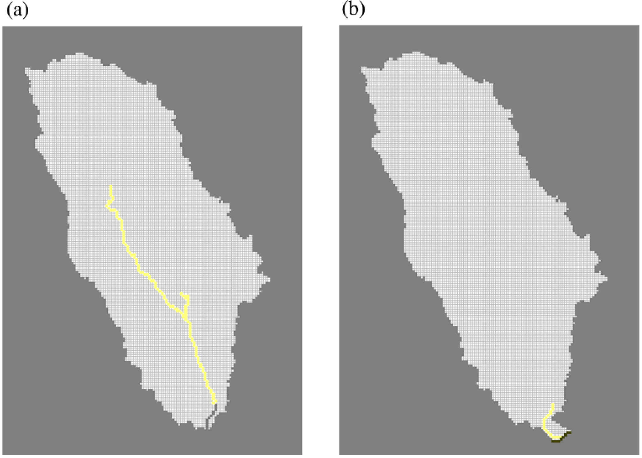
2.3. Model Setup


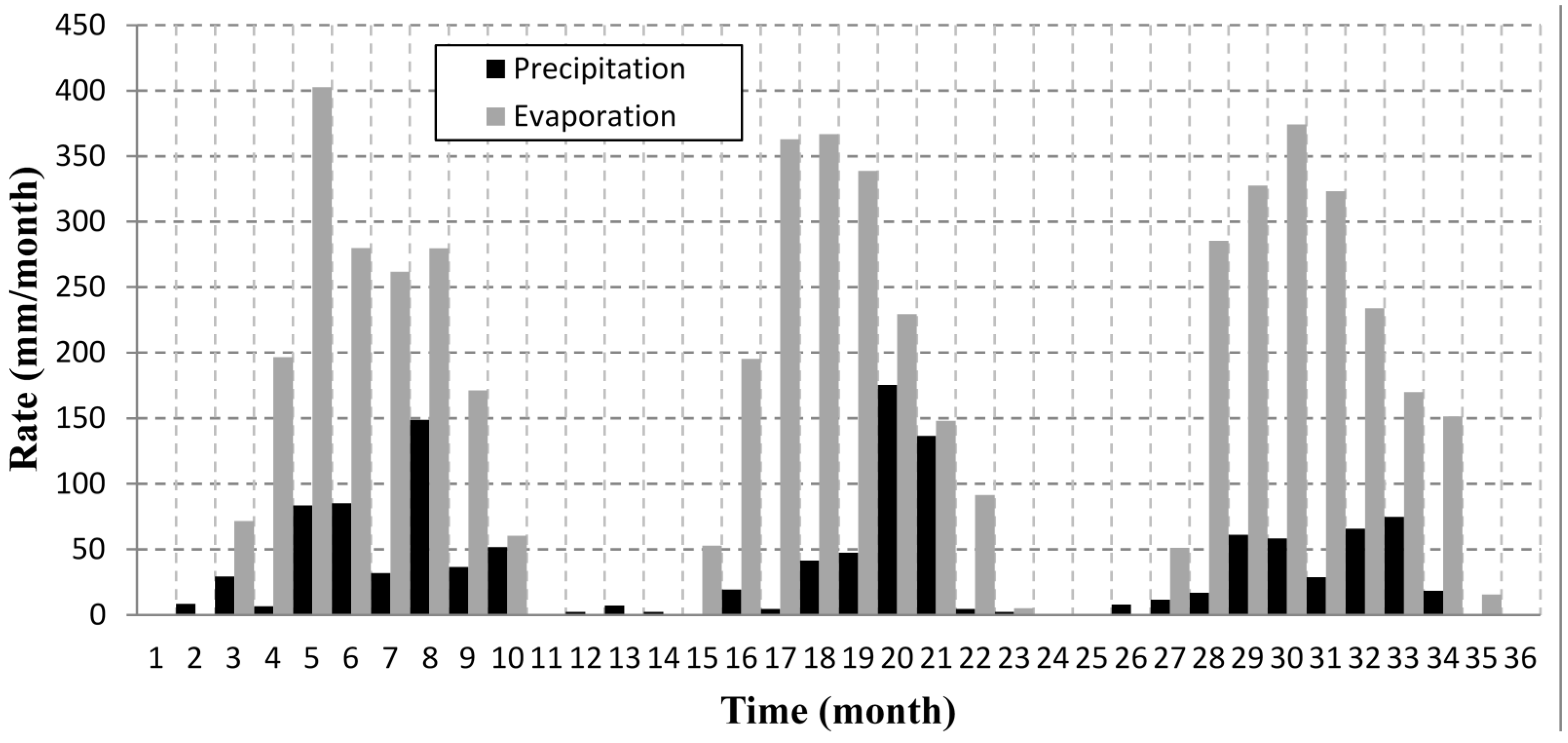
2.4. Synthetic Data Generation

| Well No. | x | y | Layer | K (m/d) |
|---|---|---|---|---|
| BH1 | 336,389.658 | 4,260,247.280 | Upper | 12.89 |
| BH2 | 332,073.543 | 4,258,013.852 | Upper | 21.47 |
| BH3 | 336,869.313 | 4,255,386.935 | Upper | 9.09 |
| BH4 | 335,747.570 | 4,251,537.000 | Bottom | 0.39 |
| BH5 | 333,485.000 | 4,251,550.000 | Upper | 17.92 |
| BH7 | 331,812.363 | 4,243,332.846 | Upper | 14.65 |
| BH8 | 337,568.173 | 4,246,870.834 | Upper | 17.12 |
| BH9 | 323,502.996 | 4,239,096.890 | Bottom | 0.077 |
| BH10 | 334,105.124 | 4,239,863.620 | Upper | 18.32 |
| BH14 | 335,747.570 | 4,226,004.390 | Upper | 5.56 |
| BH15 | 339,219.970 | 422,110.540 | Bottom | 0.066 |
| BH16 | 324,070.370 | 4,240,827.500 | Upper | 10.15 |
| BH17 | 342,183.141 | 4,252,717.435 | Upper | 15.64 |
| Model | Sill | Integral Scale/Range | NLL | KIC | Rank |
|---|---|---|---|---|---|
| Exponential | 0.200 | 10,016.06 | 9.413 | 2.491 | 1 |
| Gaussian | 0.161 | 10,975.12 | 9.184 | 4.951 | 2 |
| Spherical | 0.211 | 27,543.90 | 9.281 | 6.071 | 3 |

2.5. Multiple Conceptual Models

| Parameter | Value | Unit |
|---|---|---|
| Discretization | ||
| Row | 200 | - |
| Column | 140 | - |
| Layer | 2 | - |
| Active cell for each layer | 10,424 | - |
| Grid spacing | 500 | m |
| Number of stress periods | 36 | - |
| Number of time steps | 28–31 | d |
| Flow (based on real field data) | ||
| Horizontal hydraulic conductivity anisotropy ratio | 1 | - |
| Vertical hydraulic conductivity anisotropy ratio | 0.1 (layer 1) | - |
| 0.01 (layer 2) | - | |
| Specific yield for layer 1 | 0.1 | - |
| Specific storage for layer 2 | 1 × 10⁻⁵ | m−1 |
| Riverbed conductance | 300 (layer 1) | m2/d |
| 150 (layer 2) | m2/d | |
| Maximum ET rate | 0–0.004 | m/d |
| ET extinction depth | 4.6 | m |
| Recharge flux | 0–0.0018 | m/d |
| Synthetic true hydraulic conductivity field | ||
| Varigram model | Exponential | - |
| Mean | 0 | - |
| Variance | 0.2 (layer 1) | - |
| 0.15 (layer 2) | - | |
| Integral scale | 10,000 (layer 1) | m |
| 20,000 (layer 2) | m | |
| Measurement | ||
| Number of head measurements | 50 | - |
| Standard deviation | 10% of drawndown | m |
| The proposed multi-model EnKF | ||
| Number of ensemble members | 100 | - |
| Number of assimilation steps | 36 | - |
| Number of postulated models | 4 | - |
| Label of the postulated models (“Z” and “S” represent zone and segment, respectively) | Z6S1 | - |
| Z6S3 | - | |
| Z8S1 | - | |
| Z8S3 | - | |
3. Results and Discussion


4. Conclusions
Acknowledgments
Author Contributions
Conflicts of Interest
References
- Hill, M.C.; Tiedeman, C.R. Effective Groundwater Model Calibration: With Analysis of Data, Sensitivities, Predictions, and Uncertainty; John Wiley & Sons: New York, NY, USA, 2007; p. 480. [Google Scholar]
- Carrera, J. An overview of uncertainties in modelling groundwater solute transport. J. Contam. Hydrol. 1993, 13, 23–48. [Google Scholar] [CrossRef]
- Kitanidis, P.K. Introduction to Geostatistics: Applications in Hydrogeology; Cambridge University Press: Cambridge, UK, 1997. [Google Scholar]
- Yeh, W.W.-G. Review of parameter identification procedures in groundwater hydrology: The inverse problem. Water Resour. Res. 1986, 22, 95–108. [Google Scholar] [CrossRef]
- Ginn, T.R.; Cushman, J.H. Inverse methods for subsurface flow: A critical review of stochastic techniques. Stoch. Hydrol. Hydraul. 1990, 4, 1–26. [Google Scholar] [CrossRef]
- Gómez-Hernández, J.J.; Franssen, H.-J.H.; Sahuquillo, A. Stochastic conditional inverse modeling of subsurface mass transport: A brief review and the self-calibrating method. Stoch. Environ. Res. Risk Assess. 2003, 17, 319–328. [Google Scholar] [CrossRef]
- Hendricks Franssen, H.J.; Alcolea, A.; Riva, M.; Bakr, M.; van der Wiel, N.; Stauffer, F.; Guadagnini, A. A comparison of seven methods for the inverse modelling of groundwater flow. Application to the characterisation of well catchments. Adv. Water Resour. 2009, 32, 851–872. [Google Scholar]
- Riva, M.; Guadagnini, A.; Neuman, S.P.; Janetti, E.B.; Malama, B. Inverse analysis of stochastic moment equations for transient flow in randomly heterogeneous media. Adv. Water Resour. 2009, 32, 1495–1507. [Google Scholar] [CrossRef]
- Carrera, J.; Alcolea, A.; Medina, A.; Hidalgo, J.; Slooten, L.J. Inverse problem in hydrogeology. Hydrogeol. J. 2005, 13, 206–222. [Google Scholar] [CrossRef]
- Bond, C.E.; Gibbs, A.D.; Shipton, Z.K.; Jones, S. What do you think this is? “Conceptual uncertainty” in geoscience interpretation. GSA Today 2007, 17, 4. [Google Scholar]
- Neuman, S.P. Maximum likelihood Bayesian averaging of uncertain model predictions. Stoch. Environ. Res. Risk Assess. 2003, 17, 291–305. [Google Scholar] [CrossRef]
- Beven, K.; Binley, A. The future of distributed models: Model calibration and uncertainty prediction. Hydrol. Process. 1992, 6, 279–298. [Google Scholar] [CrossRef]
- Feyen, L.; Beven, K.J.; de Smedt, F.; Freer, J. Stochastic capture zone delineation within the generalized likelihood uncertainty estimation methodology: Conditioning on head observations. Water Resour. Res. 2001, 37, 625–638. [Google Scholar] [CrossRef]
- Freer, J.; Beven, K.; Ambroise, B. Bayesian estimation of uncertainty in runoff prediction and the value of data: An application of the GLUE approach. Water Resour. Res. 1996, 32, 2161–2173. [Google Scholar] [CrossRef]
- Hoeting, J.A.; Madigan, D.; Raftery, A.E.; Volinsky, C.T. Bayesian Model Averaging: A Tutorial. Stat. Sci. 1999, 14, 382–401. [Google Scholar] [CrossRef]
- Duan, Q.; Ajami, N.K.; Gao, X.; Sorooshian, S. Multi-model ensemble hydrologic prediction using Bayesian model averaging. Adv. Water Resour. 2007, 30, 1371–1386. [Google Scholar] [CrossRef]
- Rings, J.; Vrugt, J.A.; Schoups, G.; Huisman, J.A.; Vereecken, H. Bayesian model averaging using particle filtering and Gaussian mixture modeling: Theory, concepts, and simulation experiments. Water Resour. Res. 2012, 48, W05520. [Google Scholar]
- Tsai, F.T.-C. Bayesian model averaging assessment on groundwater management under model structure uncertainty. Stoch. Environ. Res. Risk Assess. 2010, 24, 845–861. [Google Scholar] [CrossRef]
- Rojas, R.; Feyen, L.; Dassargues, A. Conceptual model uncertainty in groundwater modeling: Combining generalized likelihood uncertainty estimation and Bayesian model averaging. Water Resour. Res. 2008, 44, W12418. [Google Scholar] [CrossRef]
- Rojas, R.; Feyen, L.; Batelaan, O.; Dassargues, A. On the value of conditioning data to reduce conceptual model uncertainty in groundwater modeling. Water Resour. Res. 2010, 46, W08520. [Google Scholar]
- Ye, M.; Neuman, S.P.; Meyer, P.D. Maximum likelihood Bayesian averaging of spatial variability models in unsaturated fractured tuff. Water Resour. Res. 2004, 40, W05113. [Google Scholar]
- Ye, M.; Meyer, P.D.; Neuman, S.P. On model selection criteria in multimodel analysis. Water Resour. Res. 2008, 44. [Google Scholar] [CrossRef]
- Neuman, S.P.; Xue, L.; Ye, M.; Lu, D. Bayesian analysis of data-worth considering model and parameter uncertainties. Adv. Water Resour. 2012, 36, 75–85. [Google Scholar] [CrossRef]
- Xue, L.; Zhang, D.; Guadagnini, A.; Neuman, S.P. Multimodel Bayesian analysis of groundwater data worth. Water Resour. Res. 2014, 50, 8481–8496. [Google Scholar] [CrossRef]
- Chen, Y.; Zhang, D. Data assimilation for transient flow in geologic formations via ensemble Kalman filter. Adv. Water Resour. 2006, 29, 1107–1122. [Google Scholar] [CrossRef]
- Hendricks Franssen, H.J.; Kinzelbach, W. Real-time groundwater flow modeling with the Ensemble Kalman Filter: Joint estimation of states and parameters and the filter inbreeding problem. Water Resour. Res. 2008, 44. [Google Scholar] [CrossRef]
- Xie, X.; Zhang, D. Data assimilation for distributed hydrological catchment modeling via ensemble Kalman filter. Adv. Water Resour. 2010, 33, 678–690. [Google Scholar] [CrossRef]
- Xue, L.; Zhang, D. A multimodel data assimilation framework via the ensemble Kalman filter. Water Resour. Res. 2014, 50, 4197–4219. [Google Scholar] [CrossRef]
- Kurtz, W.; Hendricks Franssen, H.-J.; Brunner, P.; Vereecken, H. Is high-resolution inverse characterization of heterogeneous river bed hydraulic conductivities needed and possible? Hydrol. Earth Syst. Sci. 2013, 17, 3795–3813. [Google Scholar] [CrossRef]
- Burgers, G.; van Leeuwen, P.; Evensen, G. Analysis scheme in the ensemble Kalman filter. Mon. Weather Rev. 1998, 126, 1719–1724. [Google Scholar] [CrossRef]
- Samper, F.J.; Neuman, S.P. Estimation of spatial covariance structures by adjoint state maximum likelihood cross validation: 1. Theory. Water Resour. Res. 1989, 25, 351–362. [Google Scholar] [CrossRef]
- Deutsch, C.V.; Journel, A.G. GSLIB: Geostatistical Software Library and User’s Guide, 2nd ed.; Oxford University Press Oxford: New York, NY, USA, 1998. [Google Scholar]
- Ye, M.; Pohlmann, K.F.; Chapman, J.B.; Pohll, G.M.; Reeves, D.M. A model-averaging method for assessing groundwater conceptual model uncertainty. Ground Water 2010, 48, 716–728. [Google Scholar] [CrossRef] [PubMed]
- Poeter, E.; Anderson, D. Multimodel ranking and inference in ground water modeling. Ground Water 2005, 43, 597–605. [Google Scholar] [CrossRef] [PubMed]
- Banta, E.R. MODFLOW-2000: The US Geological Survey Modular Ground-Water Model--Documentation of Packages for Simulating Evapotranspiration with a Segmented Function (ETS1) and Drains with Return Flow (DRT1), USGS Open-File Report 00–466; US Geological Survey: Reston, VA, USA, 2000. [Google Scholar]
© 2015 by the authors; licensee MDPI, Basel, Switzerland. This article is an open access article distributed under the terms and conditions of the Creative Commons Attribution license (http://creativecommons.org/licenses/by/4.0/).
Share and Cite
Xue, L. Application of the Multimodel Ensemble Kalman Filter Method in Groundwater System. Water 2015, 7, 528-545. https://doi.org/10.3390/w7020528
Xue L. Application of the Multimodel Ensemble Kalman Filter Method in Groundwater System. Water. 2015; 7(2):528-545. https://doi.org/10.3390/w7020528
Chicago/Turabian StyleXue, Liang. 2015. "Application of the Multimodel Ensemble Kalman Filter Method in Groundwater System" Water 7, no. 2: 528-545. https://doi.org/10.3390/w7020528