Article

Windows into the Recent Past: Simple Biotic Indices to Assess Hydrological Stability in Small, Isolated Ponds

Department oh Hydrobiology, Faculty of Biology, University of Warsaw at Biological and Chemical Research Centre, Żwirki i Wigury 101, 02-089 Warsaw, Poland
Water 2024, 16(9), 1206; https://doi.org/10.3390/w16091206
Submission received: 19 March 2024 / Revised: 21 April 2024 / Accepted: 22 April 2024 / Published: 24 April 2024

Abstract

:
This article presents the four biotic indices used to assess the hydrological stability of small, fishless, lowland ponds in northern Poland’s post-glacial landscape. The assessment was based on the analyses of the relative abundance of selected macroinvertebrate taxa caught using standard and non-lethal methods. The indices were derived from a multi-year analysis of data on invertebrate composition, abiotic water parameters, and publicly available satellite data. This allowed for the reconstruction of hydrological stability, including fluctuations in water level and surface area, as well as the frequency of drying, in small water bodies in the 5–10 years before sampling. The numerical relationships between the parameters describing hydrological stability and the relative abundance of several invertebrate taxa were described. A multiple regression analysis showed that hydrological stability was generally more strongly related to faunal composition than the other abiotic parameters. The indices used in this study can be a useful tool, particularly in citizen science. It is important that their numerical bases can be easily modified depending on the local conditions.

Graphical Abstract

1. Introduction

Hydroperiods (surface water duration) are a crucial aspect of wetlands, which are considered to be some of the planet’s most important ecosystems [1,2]. Small bodies of water can be seen as ‘hot-spots’ of freshwater biological diversity [3,4]. The loss of such environments leads to a significant reduction in the local biodiversity [5]. In astatic ponds, invertebrates benefit from the absence of fish, resulting in a high species richness and the presence of highly specialized taxa. The ecology of these ponds is dominated by hydrology and species interactions, particularly predation [6], especially by fish [7]. The fauna of ponds in central Europe has been studied for many years and is quite well described [8,9,10,11].
Several studies have been conducted in ponds to characterize the habitat preferences of dominant taxa and their relationships with various environmental parameters [12,13]. The species richness of different groups of macrofauna is positively correlated with the pond’s area [14,15] and its connectivity with other aquatic environments. The richness of the biota in isolated water bodies is lower than in water bodies that periodically connect with others, as noted by Meutter et al. and Jurkiewicz-Karnkowska [16,17]. Anthropogenic factors are the primary, but not the sole, driver of degradation in lowland ponds [18]. Climate change is also a significant factor affecting the functioning of biocoenosis in these ponds. Koperski [19] found a clear relationship between certain climatic parameters (i.e., the total annual amount of rainfall and snowfall, the annual number of days with precipitation and snow cover, the medium air temperature during March–November, the number of heatwaves per year) and the species composition, as well as various facets of the biodiversity of invertebrates inhabiting the ponds in this area.
Drought is a significant challenge in Poland, with more than half of the country’s area at high risk, as reported by Climate-ADAPT [20]. This phenomenon, as the average temperature increases and precipitation decreases, can lead to periodic drying up and even the complete disappearance of water bodies [21]. As a result, some groups of freshwater animals may become locally extinct [22,23]. In central Europe, there are hundreds of species that commonly inhabit this type of environment, some of which are ecologically specialized and mainly inhabit water bodies that are subject to significant fluctuations in water level and drying out. Others occur in various environments but have physiological mechanisms that enable them to complete their life cycles in small, unstable water bodies [6]. Hydrological stability refers to the persistence of relatively unchanged hydrological conditions over time [24]. Evaluating hydrological stability can be effectively achieved by assessing the cumulative effects in the ecosystem, such as diversity patterns [25,26], resulting from past hydrological changes.
Although each pond has a natural value, they are typically not subject to official forms of biological assessment. In several countries, such as in the European Union, official bio-monitoring procedures involve advanced biotic indices that are based on the taxonomic composition of various groups of freshwater organisms. These indices are used to evaluate the ecological condition of streams, lakes, and coastal waters [27]. However, similar methods for assessing ponds have not yet been implemented. Hydrological stability is an important factor in determining the ecological status of small water bodies. However, it is not the only factor. Other factors such as the chemical parameters of water, eutrophication, fish predation, the diversity and degree of anthropogenic transformation of the aquatic and riparian vegetation [28], and others also shape the composition of invertebrate assemblages [29,30]. Developing biotic indices for the assessment of the ecological condition of small water bodies is difficult due to the great diversity of abiotic parameters, even in ponds located close to each other, and their extreme variability over time [31]. However, a precise classification and functional typology of these environments, from the perspective of biodiversity conservation, will enable the development of future methods for assessing their ecological status, similar to the other types of freshwater. The methods proposed in this study are a step in this direction.

Objectives

The primary aims of this study were to:
  • quantify the hydrological stability of the ponds in lowland wetlands using simple hydrological parameters derived from the analysis of freely available maps and satellite images.
  • describe and statistically confirm the relationships between hydrological stability over several decades and the taxonomic composition of the freshwater macroinvertebrates inhabiting them.
  • determine the importance of hydrological stability in relation to the other abiotic parameters in the studied water bodies for the taxonomic composition of the macrofauna.
  • develop and test protocols for the multimetric biotic indices to reconstruct the hydrological stability of small reservoirs over several decades. It was assumed that the indices will be formatted to allow for their improvement and adaptation to other similar environments.
  • an additional aim of the study was to assess whether the non-lethal methods of obtaining information on the taxonomic composition of invertebrates could be sufficiently effective in assessing the hydrological stability of ponds.
To assess the hydrological status of the ponds, it was necessary to analyze the abundance and taxonomic composition of their fauna. Despite the availability of satellite data, archived remote sensing data for some of the areas was difficult to access and often had a low resolution. High-resolution data is usually offered for a fee and with a delay. Remote sensing data was available for the different areas of the globe with varying intensities. Assessing the current hydrological status based on the satellite data of small ponds, especially those surrounded by dense and tall vegetation, can be difficult or even impossible. The proposed indices can also be used as an element of citizen science, which is widely discussed and increasingly emphasized in nature conservation and social education [32,33,34]. The Supplementary Materials include executable files (File S1) and an interactive key for identifying the taxa used to calculate the proposed indices (File S2). Their use is currently limited to the lowland areas of Central Europe.

2. Materials and Methods
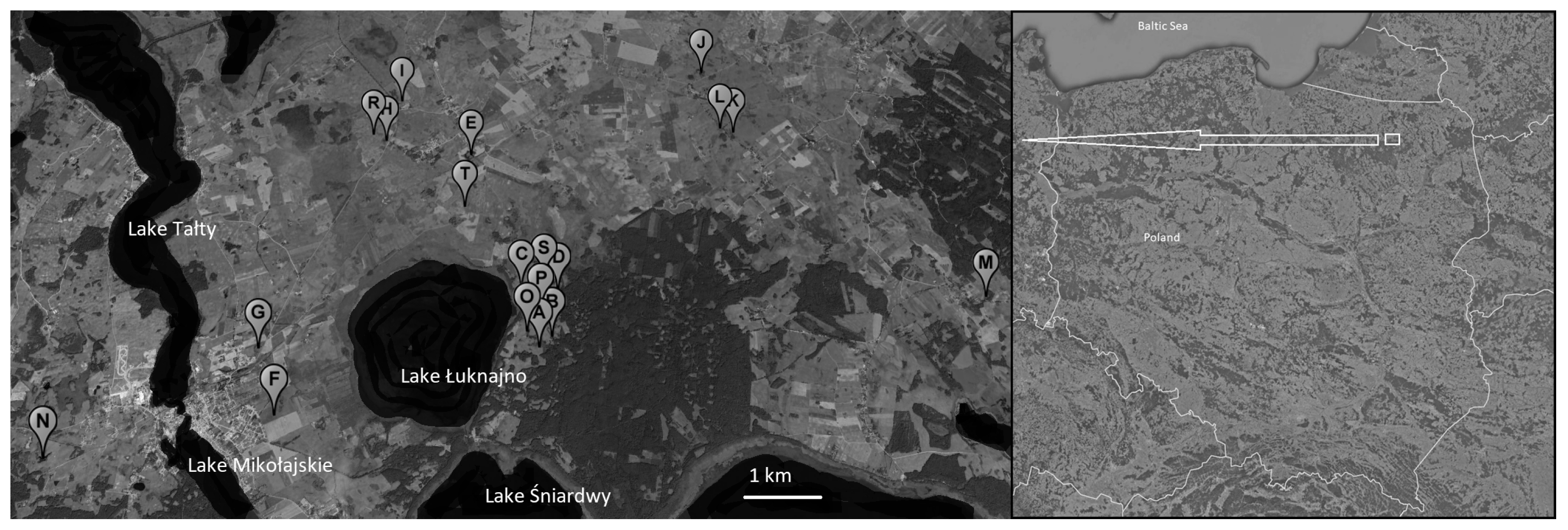
2.1. Study Area

The study area consisted of a fragment of vast, strongly fragmented, and partially degraded wetlands located in the post-glacial lake district in north-eastern Poland, near the Łuknajno, Śniardwy, and Mikołajskie lakes (Figure 1). This area is protected as part of the Masurian Landscape Park. The certain studied ponds were located in the buffer zone of the UNESCO Biosphere Reserve (since 1972) and have also been protected by the Ramsar Convention since 1977 [35]. The areas under study were previously heavily utilized for agriculture. Currently, these areas are mainly semi-natural fallow lands, grasslands, and bushes, some of which are mown once a year to stop overgrowing. The region contains numerous permanent and temporary small water bodies, which have been significantly impacted in recent years by the changing hydrological conditions [19]. Since 2009, a water retention program has been implemented in the vicinity of the Puszcza Piska Forest (a forest complex covering an area of approximately 1000 km2, which is currently highly fragmented), resulting in significant hydrological changes in the neighboring post-agricultural area.

2.2. Sampling

Data on the hydrological stability and the fauna inhabiting 19 small, shallow, fishless ponds isolated from other water bodies (Figure 1) were collected. The ponds had an average surface area of between 200 and 25,000 m2 and a maximum depth of 0.5–1.8 m during the study. The average distance between the ponds was 4.02 km, and the greatest distance between two ponds was approximately 12 km. The abiotic parameters of the water were measured concurrently with the faunistic samples three or four times in 2010–2011 and twice in 2017–2018 in each pond (refer to Figure 2). The analyses conducted in 2010–2011 were performed in the Laboratory of Environmental Chemistry at the University of Warsaw in accordance with the Polish Norms for water chemistry. In 2017–2018, multi-parameter Corning Checkmate equipment and a Merck Spectroquant Nova 60 photometer were used [19].
In May and June between 2010 and 2019, samples of invertebrates were collected from two different sampling points in each pond using a semi-quantitative dip net method (1.0 mm mesh size). The dip net was dragged just above the bottom, outside the dense vegetation, for 10 drags, each time covering a distance of 1.5 m. The collected material was preserved with ethyl alcohol. The effectiveness of the assessment was also tested using non-lethal samples of fauna (photographs were taken). In 2014, samples were taken from 14 sites using both traditional and photographic methods to assess the taxonomic composition. The photographic method does not cause the death of the collected animals and is faster and easier to learn (although animal identification is less accurate than traditional methods); therefore, it is more convenient as part of citizen science procedures. The selected taxonomic groups were confirmed to be present in the fauna samples using both methods. A comparison was made between the effectiveness of assessing the taxonomic composition using traditional and photographic methods. The taxonomic groups selected for the next steps of the analysis were those whose presence in the fauna samples was confirmed using both methods.
Thirteen parameters describing hydrological stability were used to recreate the past values. These included the variability of the pond surface area in the 3, 5, and 10 years prior to sampling (expressed as the standard deviation), the average pond surface area in the 1, 3, 5, and 10 years prior to sampling (expressed as a percentage of the maximum surface area), and the number of years in which episodes of complete drying of the pond were recorded in the 10 and 35 years prior to sampling. The following two parameters were recorded: the smallest pond surface area in the 5, 10, and 20 years prior to sampling, expressed as a percentage of the maximum surface area during the past 20 years; and the time (in years) that has passed since the last reduction of the pond to 20% of its maximum area.
The surface area data for the studied water bodies were obtained solely from open-access databases. This included an analysis of approximately 760 historical satellite images from sources such as Google Earth Pro, Google Earth Time Lapse, Land Sat Viewer, and Geoportal (https://mapy.geoportal.gov.pl/, accessed on 15 April 2024). Additionally, around 170 topographic and satellite maps from Geoportal were analyzed. Field measurements of the pond surface area taken between 2010 and 2019 were also utilized. When encountering low-resolution photos, the ‘Digimizer’ application was used to extrapolate the surface with an accuracy of 10% of the maximum surface. The analysis was conducted using photos and maps taken during the periods of the lowest water levels, specifically in August and September.
Changes over time were found to be correlated with the changes in the taxonomic composition of the aquatic macroinvertebrates. The strength of the linear correlation between the values of the hydrologic and taxonomic parameters was calculated. This included the percentages of phyla, orders, families, and in some cases, genera or species, as well as the basic measures of taxonomic diversity of the fauna in the samples, such as the Shannon and Margalef diversity indices, the taxonomic richness, and the estimated taxonomic richness using the Chao1 function values.

2.3. Testing the Significance of Abiotic Parameters

This study analyzed the relationship between the relative abundance of the 16 most common taxonomic groups of macroinvertebrates and the abiotic parameters measured in the studied ponds. To achieve this, 16 multiple regression models were created based on the normalized values of these parameters. Fourteen models had a multiple regression coefficient, R2, exceeding 0.3 and were considered significant based on a p-value below 0.05 for the t-test. In all models, the hydrological stability indicators (described in detail below) were highly significant variables. They were of the greatest significance, as expressed by the highest values of the Beta coefficient (describing the strength of the relationship) or the partial multiple regression coefficients (indicating the share of a given factor in the explanatory power model) (File S3). In certain models, the surface area of the pond, the nutrient content, and the electrolytic conductivity were significant factors.

2.4. Data Preparation for Hydrological Stability Assessment

To assess the hydrological stability, a multiple stepwise regression model with backward elimination was created for each hydrological parameter. Only the taxonomic parameters with statistically significant linear correlation coefficients at the p < 0.05 level were used. The taxonomic groups represented by the explanatory variables, whose presence or identification was not confirmed using photographic analysis, such as Limnephilidae, Hydrophilidae, Oligochaeta, Dixidae, Haliplidae, Helodidae, Limoniidae, Plea minutissima, and Tabanidae, were removed.
The indices were developed and tested to assess the hydrological parameters based on the taxonomic composition of the macroinvertebrates. The procedure below allowed for the obtaining of precise information on the basic parameters that describe the hydrological stability of the ponds within the 5–10 years before the sampling of the macroinvertebrates.
  • The hydrological parameters were normalized.
  • Taxa that were found to have a significant explanatory power in the multiple regression models at a level of p < 0.05 were included in the constructed index after normalization and then (Figure 3),
  • multiplied by the R2 values in the multiple regression model. The resulting values were assigned a positive or negative value based on their relationship with the hydrological parameter.
  • The index value was obtained by taking the weighted average (the weights were determined by the R2 values) of the standardized values from point c., which were then placed on a scale of 0–1.
The following section describes the methods for calculating the proposed indices. Any index values obtained below 0 were considered as 0, and any values above 1 were considered as 1. Modifications were introduced to the formulas used to calculate all the indexes based on the samples taken and analyzed using the traditional method (analysis using a stereo-microscope after preserving the animals) and should be applied to the samples analyzed using the photographic method. The values used in the formulas were determined using the over-representation or under-representation of the taxonomic groups in the samples analyzed from the photographs compared with those analyzed after the animals had been killed and preserved. The Supplementary Materials (File S1) contain files that enable the calculation of all the presented indices based on the percentage data.
The proposed protocols were tested to better reconstruct the hydrological stability of the ponds over several decades. The proposed indices were developed based on a large dataset. A total of 48,607 individuals were identified in 75 samples collected from 19 ponds. However, this number of samples may be insufficient to draw general and far-reaching conclusions. To test the effectiveness of assessing the hydrological parameters using the described methods, a set of pseudo-samples was created. The online software ‘normally distributed random numbers generator’ (available at: https://planetcalc.com/5840/, accessed on 15 April 2024) was used. One hundred pseudo-samples were generated for each of the four categories of values for each of the four indicators, resulting in a total of 1600 pseudo-samples, based on the original, real data on the number of taxa in the samples. For each pseudo-sample, the number of each indicative taxon was generated based on the normal distribution of the original values in the samples from a given category. The frequency of the occurrence of zero values and single individuals in the sample (singletons) corresponded to the frequency of their appearance in the original samples from each category.
The species composition data from the traditional and photographic methods were analyzed using PCA with in-variance/covariance mode (PAST 4.03 software). The analyzed variables were the percentages of the taxa. A comparison was conducted to evaluate the differences in the hydrological stability assessment results using both versions of the proposed indices for lethal and non-lethal sampling.

3. Results

Significant variability in time was found in the parameters describing the hydrological stability of the individual ponds. Those parameters were used to quantify the hydrological stability of the ponds. The average dominant trend (a polynomial relationship of the second degree) showed that this was highest around 2015 and clearly lower before and after (see Figure 4).
Of the 13 tested hydrological parameters, the models for three of them explained a significant part of the overall variability (parameter R2adj > 0.7):
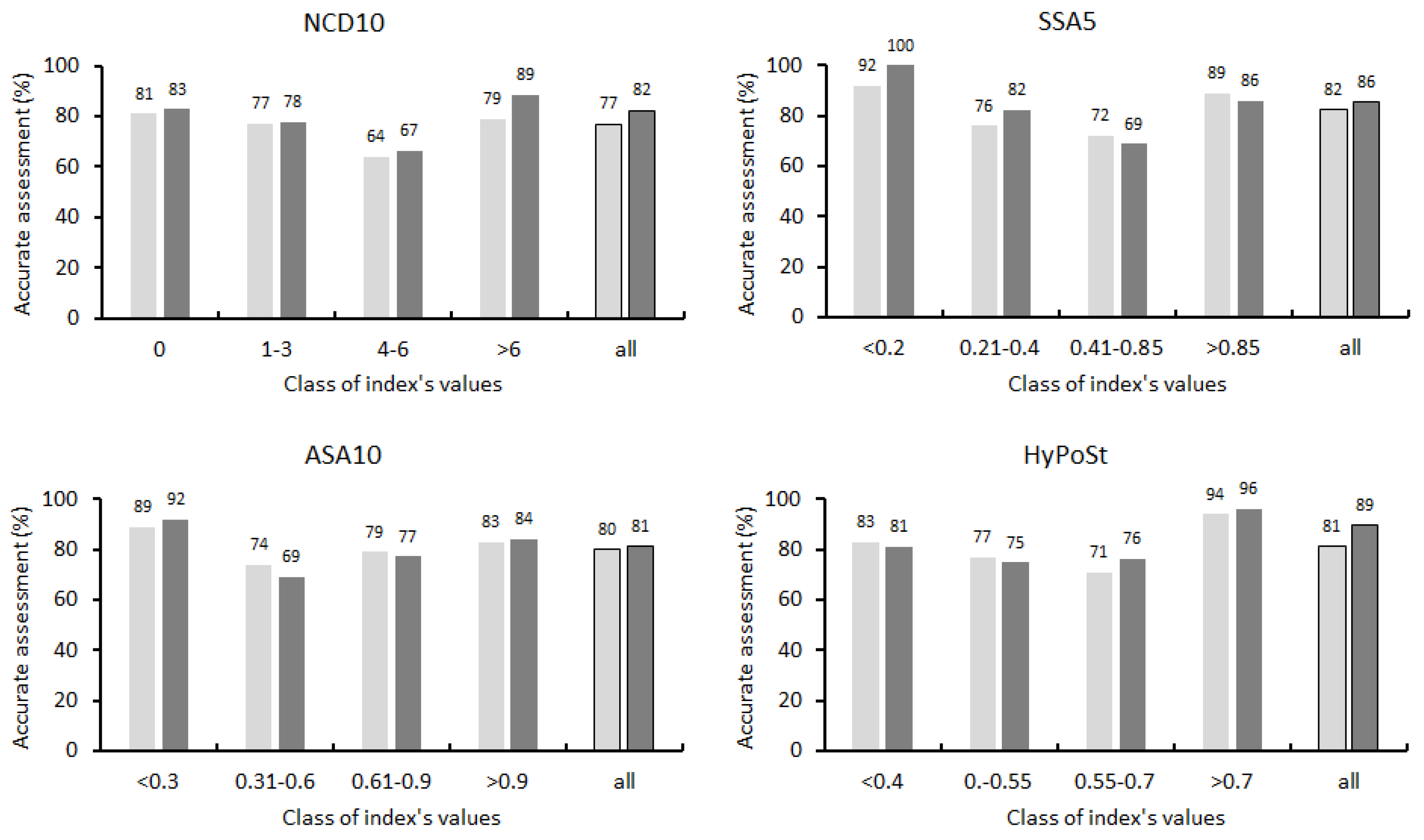
  • The average pond surface area during the 10 years prior to sampling, expressed as a percentage of the maximum surface area (ASA10) on a scale of 0–1.
  • The number of years in which episodes of complete drying of the pond were recorded during the 10 years prior to sampling (NCD10) on a scale of 0–10.
  • The smallest recorded pond surface area in the 5 years prior to sampling, expressed as a percentage of the maximum surface area during the past 20 years (SSA10) on a scale of 0–1.
All the proposed indices were based on the relative abundance of the taxa, with high indicative values in terms of the parameters describing hydrological stability (Figure 3). Statistically significant differences were found between the values of each index used to determine the hydrological parameters in the past, which were classified into different classes (see Table 1).
Additionally, the differences between the values of the hydrological stability parameters, calculated based on the indices’ values classified into different classes, were also statistically significant (see Table 2).

3.1. The Indices

(1) To assess the average pond surface area over the 10 years prior to sampling, expressed as a percentage of the maximum surface area (ASA10), the ASAMi index was developed based on the percentages in the sample of three insect families: Baetidae (%Ba), Chaoboridae (%Ch), and Dytiscidae (%Dy); the genus Stagnicola (Gastropoda) (%St); the species Segmentina nitida (Gastropoda) (%Sn); and two species of Hirudinea—Erpobdella testacea (%Et) and Hirudo medicinalis (%Hm). The formula used to calculate this was:
ASAMi = (Sum1/Σ1R2 + 0.879)/2.02
where:
Sum1 = (%Ba ∙ −0.0179 + 0.219) + (%Ch ∙ −0.023 + 0.047) + (%Dy ∙ −0.059 + 0.132) +
(%St ∙ −0.173 + 0.048) + (%Sn ∙ −0.013 + 0.167) + (%Et ∙ 0.040 − 0.032) + (%Hm ∙ 0.248 − 0.066)
Σ1R2 is the sum of the weighed coefficients of the multiple regression for each group included in the model and is equal to 0.979.
The index used to calculate the version based on the samples analyzed with the use of the non-lethal photographic method was as follows:
ASAMi(nl) = Sum2(nl)/Σ1R2 + 1.124)/1.738
Sum1(nl) = (%Ba ∙ −0.017 + 0.209) + (%Ch ∙ −0.019 + 0.038) + (%Dy ∙ −0.048 + 0.107) +
(%St ∙ −0.148 + 0.041) + (%Sn ∙ −0.011 + 0.139) + (%Et ∙ 0.032 − 0.026) + (%Hm ∙ 0.186 − 0.050)
Based on the values of the ASAMi(tp) and the ASAMi(nl), the corresponding average pond surface area over the 10 years prior to the sampling can be estimated, expressed as a percentage of the maximum surface area (ASA10). For this purpose, the table in the appropriate sheet in (File S1) can be used.
(2) To assess the approximate number of years in which episodes of complete drying of the pond were recorded in the 10 years prior to sampling (NCD10), the NCDMi index was developed, based on the percentages in the sample of four insect families: Baetidae (%Ba), Chaoboridae (%Ch), Lestidae (%Le), and Stratiomyidae (%Str); the insect genus Notonecta (%No); and the leeches—family Glossiphonidae (%Gl) and the leech species Dina lineata (%Dl) and E. testacea (%Et). The formula used to calculate this was:
NCDMi = (Sum2/Σ2R2 + 0.789)/2.285
where:
Sum2 = (%Ba ∙ 0.028 − 0.355) + (%Ch ∙ 0.016 − 0.039) + (%Le ∙ −0.033 + 0.017) + (%Str ∙ −0.177 +
0.082) + (%No ∙ 0.033 − 0.0388) + (%Gl ∙ −0.043 + 0.038) + (%Dl ∙ 0.192 − 0.020) + (%Et ∙ 0.0413 − 0.0323)
Σ2R2 is the sum of the weighed coefficients of the multiple regression for each group included in the model and is equal to 0.899.
The index used to calculate the version based on the samples analyzed with the use of the non-lethal photographic method was as follows:
NCDMi(nl) = Sum2(nl)/Σ2R2 + 0.393/1.014
where:
Sum2(nl) = (%Ba ∙ 0.027 − 0.339) + (%Ch ∙ 0.013 − 0.031) + (%Le ∙ −0.030 + 0.016) +
(%Str ∙ −0.227 + 0.106) + (%No ∙ −0.025 − 0.029) + (%Gl ∙ −0.057 + 0.050) + (%Dl ∙ 0.168 − 0.018) + (%Et ∙ 0.033 − 0.026)
Based on the values of the NCDMi(tp) and the NCDMi(nl), the corresponding approximate number of years in which the episodes of complete drying of the pond were recorded in the 10 years prior to sampling (NCD10) can be estimated. For this purpose, the table in the appropriate sheet in (File S1) can be used.
(3) To assess the smallest surface area of a pond recorded in the 5 years prior to sampling, expressed as a percentage of the maximum surface area (SSA5), the SSAMi index was developed, based on the percentages in the sample of six insect families: Baetidae (%Ba), Chaoboridae (%Ch), Dystiscidae (%Dy), Ceratopogonidae (%Ce), Caenidae (%Ca), and Gyrinidae (%Gy); the genus Stagnicola (Gastropoda) (%St); and the species Hirudo medicinalis (Hirudinea) (%Hm). The formula used to calculate this was:
SSAMi = (Sum3/Σ3R2 + 0.842)/2.25
where:
Sum3 = (%Ba ∙ −0.069 + 0.857) + (%Ch ∙ −0.154 + 0.376) + (%Dy ∙ −0.412 + 0.9) + (%Ce ∙ 2.47 − 0.341) + (%Ca ∙ 0.437 − 0.521) + (%Gy ∙ 3.423 − 0.368) + (%St ∙ −1.457 + 0.345) + (%Hm ∙ 1.246 − 0.388)
Σ3R2 is the sum of the weighed coefficients of the multiple regression for each group included in the model and is equal to 1.64.
The index used to calculate the version based on the samples analyzed with the use of the non-lethal photographic method was as follows:∙
SSAMi(nl) = (Sum3(nl)/Σ3R2 + 3.839)/8.92
where:
Sum3(nl) = (%Ba ∙ −0.065 + 0.818) + (%Ch ∙ −0.123 + 0.302) + (%Dy ∙ −0.333 + 0.726) + (%Ce ∙ 1.709 − 0.236) + (%Ca ∙ 0.396 − 0.472) + (%Gy ∙ 2.768 − 0.298) + (%St ∙ −1.128 + 0.267) + (%Hm ∙ 2.768 − 0.297)
Based on the values of the SSAMi(tp) and the SSAMi(nl), the corresponding smallest surface area of a pond recorded in the 5 years prior to sampling can be estimated, expressed as a percentage of the maximum surface area (SSA5). For this purpose, the table in the appropriate sheet in (File S1) can be used.
(4) General Hydrological Pond Stability, The HyPoSt is a parameter that combines the three parameters mentioned above (ASA10, NCD10, and SSA5) and describes the overall hydrological stability of the pond over the past years. Its values are the normalized and standardized arithmetic mean of the ASA10, NCD10, and SSA5 values of each reservoir in each year.
To calculate it, use the formula:
HyPoSt(norm) = (ASA10 ∙ 0.039 − 2.427) + (NCD10 ∙ −0.389 + 1.157) + (SSA5 ∙ 0.029 − 1.159))/3 and standardize the obtained values according to the formula:
HyPoSt = (HyPoSt(norm) + 0.036)/0.991
To evaluate the HyPoSt, the HyPoStMi index was developed, based on the percentages in the sample of five insect families—Baetidae (%Ba), Chaoboridae (%Ch), Gyrinidae (%Gy), Caenidae (%Ca), and Coenagrionidae (%Co); the genus Stagnicola (Gastropoda) (%St); and the species H. medicinalis (Hirudinea) (%Hm). The formula used to calculate this was:
HyPoStMi = (Sum4/Σ4R2 + 0.155)/0.295, where Sum4 = (%Ba ∙ −0.09 + 0.221) + (%Ch ∙ −0.016 + 0.059) + (%Gy ∙ 0.114 − 0.027) + (%Co ∙ 0.022 − 0.070) + (%Ca ∙ 0.014 − 0.054) + (%St ∙ −0.073 + 0.037) + (%Hm ∙ 0.025 − 0.041)
Σ4R2 is a sum of the weighed coefficients of the multiple regression for each group included in the model and is equal to 0.992.
The Sum4 parameter used to calculate the indicator version based on the samples analyzed using the HyPoStMi(nl) photographic method had the following form:
Sum4(nl) = (%Ba ∙ −0.008 + 0.207) + (%Ch ∙ −0.0.013 + 0.048) + (%Gy ∙ 0.092 − 0.022) + (%Co ∙ 0.018 − 0.056) + (%Ca ∙ 0.013 − 0.050) + (%Aa ∙ 0.005 − 0.075) + (%St ∙ −0.063 + 0.032) + (%Hm ∙ 0.019 − 0.031)
Based on the values of the HyPoStMi(tp) and the HyPoStMi(nl), the corresponding overall hydrological stability of the pond over the past years (HyPoSt) can be estimated. For this purpose, the table in the appropriate sheet in (File S1) can be used.

3.2. Testing the Indices Using Descriptive Statistics

The drawn numbers of the individual taxa were randomly matched using a pseudorandom number generator in the Excel software package. This study employed pseudo-samples to simulate the samples taken from similar ponds with a comparable location and morphometry. The proposed indices were used to predict the parameters describing hydrological stability, and the efficiency of this method was found to be high. The highest efficiency was observed for the lowest and highest classes of values for each parameter, as shown in Figure 5.
The results obtained from the indices based on the non-lethal sampling procedure were comparable to those obtained using traditional methods. Only 2 out of the 56 compared values (3.7%) showed differences in prediction exceeding 20%, and in 10 out of the 56 comparisons (17.9%), the differences exceeded 10% (refer to Figure 6).
The data on the composition of macroinvertebrates obtained using both traditional and non-lethal methods were similar. Both sets of samples on the ordination map almost completely overlapped (eigenvalues were 2.75 and 1.13 for PC1 and PC2, respectively, as shown in Figure 7).

4. Discussion

The temporal variability of hydrological stability, as read from the analyzed data (approximated as a second-degree polynomial relationship), is generally consistent with the data on transpiration and precipitation in this area during the studied period [19]. The warming observed in the various regions of the globe in the past 30 years is linked to the global temperature increases. However, in the past two decades, the average temperature increase in Poland has exceeded the global average by 0.03 °C per year. Climate change in Poland is evidenced by the increasing average annual and seasonal air temperatures, the annual and seasonal maximum air temperatures, the number of hot days and heatwaves, and the decreasing number of frosty days. There has been an important change in the number of weather types per year, as reported by Falarz et al. [36]. Additionally, there has been a change in the intensity of precipitation in most of Poland, with the length of the precipitation-free period extended by up to 5 days per decade, according to Łupikasza and Małarzewski [37]. The question of universality arises—how reliable are the developed indices when used in other water bodies? The bioindicators used to construct these groups are commonly found in small, hydrologically isolated, shallow, unpolluted, lowland ponds in central Europe. These ponds typically have a neutral water pH and contain insignificant amounts of humic compounds. The taxonomic composition of the macrofauna in similar European water bodies may vary locally, but generally includes a similar list of taxa [14,38,39]. The changes in hydrological stability can have a significant impact on the taxonomic composition and diversity of the macroinvertebrates in small ponds. However, predicting these effects is not always straightforward. Recent studies by Epele et al. [40,41] suggest that factors such as air temperature and seasonal changes in precipitation intensity may play a role in determining the differences in taxonomic composition between similar wetland types. As periodic drying out occurs more frequently, it is expected that more resistant species will replace the more sensitive ones in a shorter time frame, rather than a significant reduction in species richness [42,43]. This study presents the important bio-indicators, which are the dominant taxa. These include several families of insects, such as mayflies, true flies, beetles, and damselflies, as well as several species of leeches and lung-breathing snails. It is necessary to test these indices in other small, fishless reservoirs with a similar location, origin, morphometry, and hydrochemistry.
Invertebrates exhibit significant variation in their biology and adaptations that allow them to inhabit small, astatic ponds either permanently or temporarily. The taxonomic composition of these invertebrates can also serve as an indicator of the type and intensity of anthropogenic pressure [29,44]. Notably, the larvae of Baetidae and Chaoboridae are of particular importance, as their high percentages in the samples suggest a low hydrological stability of the pond. The most prevalent species of Chaoboridae found in the samples was Chaoborus crystallinus, accounting for over 97% of all the identified specimens in the samples. This species is known for its ability to expedite the development of larval stages in small water bodies, resulting in up to four generations appearing during the growing season [45]. The Baetidae species that are most commonly found in small reservoirs are known for their early spring emergence. Their ovo-viviparity enables them to quickly rebuild their population numbers after a catastrophic drying out [46]. The presence of high percentages of Hirudo medicinalis and Caenidae and Stratiomyidae larvae indicates that the pond has high hydrological stability. Some taxa have a significant indicative value in determining one or several of the proposed indices but are of little significance in relation to the other values. For instance, a high percentage of Dystiscidae beetles correlates well with a low hydrological stability expressed by the SSA5 and ASA10 parameters, but it is not significantly related to the NCD10 values. The absence of a correlation with the latter can be explained by the fact that most Dytiscidae species’ adults are proficient flying insects, effectively and rapidly colonizing the reservoirs that are recovering after a catastrophic drying out [47]. The NCD10 value directly describes the frequency of a catastrophic, complete drying out, which appears to have a particularly strong impact on the occurrence of species with a limited ability to actively colonize ponds. This seems to explain the significance of the leeches Erpobdella testacea, Dina lineata, and Glossiphonidae as component metrics of the NCDMi index.
Evaluating a pond’s past stability can provide important insights into its future stability, taking into account the intensifying effects of climate change. This includes the increasing frequency of small water bodies disappearing, the prolonged heatwaves, and the rainfall shortages [19,35,36]. Accurately predicting the stability of the ponds is crucial for planning environmental management projects that utilize small bodies of water as protected areas and refuges for rare and protected species. This information can be used to identify habitat management priorities, such as assessing the suitability of the habitat for protected species of amphibians [48], fish [49], and birds [31].
By following the described methodology, the user can collect a sample of macroinvertebrates. The macroinvertebrate samples can then be identified using the associated key (Additional Materials B) and the application provided in this article (Additional Materials A). This process provides valuable information about the sampled pond. For instance, if the animals sampled consisted of 35% mayflies from the Baetidae family, 24% Segmentina nitida snails, 15% Chaoboridae, and 1% Caenidae, the pond has had a low overall hydrological stability in recent years (HyPoSt index of 0.171). The water surface area has been below average, less than 30% of the maximum (ASA10 0.301), and the minimum water surface area has been less than 20% of the maximum (SSA5 0.264). Additionally, the pond has dried out completely at least six times in the past ten years (NCD 0.77). If a non-lethal method was used to collect this sample, the hydrological parameter values would differ only slightly. Only for ASA10 would a higher class of values be obtained, resulting in an average water surface in the reservoir of 30–60% of the maximum. It is assumed that the described indices will be formatted to allow for their improvement and adaptation to other similar environments by other scientists. It should be emphasized that the presented assessment methods can be applied to small, natural, or semi-natural shallow ponds in the lowland areas of Central Europe. Analysis in other geographic regions and other pond types will require additional research, including primary faunistic studies and the standardization of differences in the abundance of taxonomic groups between ponds with different hydroperiods.
The use of the proposed indices as an element of citizen science appears to be a suitable and highly beneficial method for assessing the recent hydrological past of ponds. The identification key and calculation file (Files S1 and S2) make the non-lethal version relatively easy, fast, and inexpensive, even for those without expert knowledge in biological monitoring. The proposed indices enable easy and quick recognition of the fundamental hydrological parameters of these water bodies. They can be considered as windows into the recent past of these valuable natural environments, while taking into account local time and space constraints.

Supplementary Materials

The following supporting information can be downloaded at: https://www.mdpi.com/article/10.3390/w16091206/s1, File S1. Indices. Executable file to calculate values of indices; File S2. Key. Key to identification of taxa used to calculate indices; File S3. MultiReg. Formulas and parameters used to prepare models of multiply regression.

Funding

This research was partially funded by the National Science Center of Poland, grant number NCN 2011/01/B/NZ9/02590.

Data Availability Statement

All data that may be freely available due to privacy and ethical constraints are included in the text and in the Supplementary Materials.

Acknowledgments

Some of the data used in this publication were collected during the field course “Flora and Fauna”, organized by the Faculty of Biology at the University of Warsaw and for the bachelor thesis of Ewa Narożniak. I would like to thank them for their cooperation. Most of the data from 2013–2014 were obtained for the Ph.D. thesis conducted at the Faculty of Biology, University of Warsaw. The author is grateful to Tomasz Karasek, who put a lot of work and ingenuity into collecting these samples, identifying the animals, and analyzing the data.

Conflicts of Interest

The author declares no conflicts of interest.

References

  1. Céréghino, R.; Biggs, J.; Oertli, B.; Declerck, S. The ecology of European ponds: Defining the characteristics of a neglected freshwater habitat. Hydrobiology 2008, 597, 1–6. [Google Scholar] [CrossRef]
  2. Gökçe, D. Wetland importance and management. In Wetlands Management—Assessing Risk and Sustainable Solutions; Gökçe, D., Ed.; IntechOpen: London, UK, 2019. [Google Scholar] [CrossRef]
  3. Scheffer, M.; Van Geest, G.J.; Zimmer, K.; Jeppesen, E.; Søndergaard, M.; Butler, M.G.; De Meester, A.L. Small habitat size and isolation can promote species richness: Second-order effects on biodiversity in shallow lakes and ponds. Oikos 2006, 112, 227–231. [Google Scholar] [CrossRef]
  4. Oertli, B.; Parris, K.M. Toward management of urban ponds for freshwater biodiversity. Ecosphere 2019, 10, e02810. [Google Scholar] [CrossRef]
  5. Horváth, Z.; Ptacnik, R.; Vad, C.F.; Chase, J.M. Habitat loss over six decades accelerates regional and local biodiversity loss via changing landscape connectance. Ecol. Lett. 2019, 22, 1019–1027. [Google Scholar] [CrossRef]
  6. Jeffries, M.J.; Epele, L.B.; Studinski, J.M.; Vad, C.F. Invertebrates in Temporary Wetland Ponds of the Temperate Biomes. In Invertebrates in Freshwater Wetlands; Batzer, D., Boix, D., Eds.; Springer: Cham, Switzerland, 2016. [Google Scholar] [CrossRef]
  7. Nieoczym, M.; Stryjecki, R.; Buczyński, P.; Płaska, W.; Kloskowski, J. Differential abundance, composition and mesohabitat use by aquatic macroinvertebrate taxa in ponds with and without fish. Aquat. Sci. 2023, 85, 25. [Google Scholar] [CrossRef]
  8. Harper, D.; Mekotova, J.; Hulme, S.; White, J.; Hall, J. Habitat heterogeneity and aquatic invertebrate diversity in floodplain forests. Glob. Ecol. Biogeogr. 1997, 6, 275–285. [Google Scholar] [CrossRef]
  9. Buczyńska, E.; Buczyński, P.; Lechowski, L.; Stryjecki, R. Fish pond complexes as refugia of aquatic invertebrates (Odonata, Coleoptera, Heteroptera, Trichoptera, Hydrachnidia): A case study of the pond complex in Zalesie Kańskie (Central-East Poland). Nat. Conserv. 2007, 64, 39–55. [Google Scholar]
  10. Biggs, J.; Bilton, D.; Williams, P. Temporary pond of eastern Poland: An initial assessment of their importance for nature conservation. Arch. Sci. 2004, 57, 73–84. [Google Scholar] [CrossRef]
  11. Bloechl, A.; Koenemann, S.; Philippi, B.; Melber, A. Abundance, diversity and succession of aquatic Coleoptera and Heteroptera in a cluster of artificial ponds in the North German Lowlands. Limnologica 2010, 40, 215–225. [Google Scholar] [CrossRef]
  12. Briers, R.A.; Biggs, J. Indicator taxa for the conservation of pond invertebrate diversity. Aquat. Conserv. 2003, 13, 323–330. [Google Scholar] [CrossRef]
  13. Céréghino, R.; Boix, D.; Cauchie, H.M.; Martens, K.; Oertli, B. The ecological role of ponds in a changing world. Hydrobiologia 2014, 723, 1–6. [Google Scholar] [CrossRef]
  14. Oertli, B.; Joye, D.A.; Castella, E.; Juge, R.; Cambin, D.; Lachavanne, J.B. Does size matter? The relationship between pond area and biodiversity. Biol. Cons. 2002, 104, 59–70. [Google Scholar] [CrossRef]
  15. Koperski, P.; Narożniak, E.; Mętrak, M. Composition of mollusk communities as a proxy in studies on seasonal dynamics of astatic water bodies. Monit. Środ Przyr. 2014, 15, 23–31. [Google Scholar]
  16. Meutter, F.V.D.; Meester, L.D.; Stoks, R. Metacommunity structure of pond macroinvertebrates: Effects of dispersal mode and generation time. Ecology 2007, 88, 1687–1695. [Google Scholar] [CrossRef]
  17. Jurkiewicz-Karnkowska, E. Effects of habitat conditions on the diversity and abundance of molluscs in floodplain water bodies of different permanence of flooding. Pol. J. Ecol. 2011, 59, 165–178. [Google Scholar]
  18. Ostad-Ali-Askari, K. Review of the effects of the anthropogenic on the wetland environment. Appl. Water Sci. 2022, 12, 260. [Google Scholar] [CrossRef]
  19. Koperski, P. Hydrological instability of ponds reduces functional diversity of freshwater molluscs in protected wetlands. Wetlands 2022, 42, 42. [Google Scholar] [CrossRef]
  20. CLIMATE-ADAPT. Available online: https://climate-adapt.eea.europa.eu/en/countries-regions/countries/poland (accessed on 15 March 2021).
  21. Matthews, J. Anthropogenic climate change impacts on ponds: A thermal mass perspective. BioRisk 2010, 5, 193–209. [Google Scholar] [CrossRef]
  22. Lund, J.O.; Wissinger, S.A.; Peckarsky, B.L. Caddisfly behavioral responses to drying cues in temporary ponds: Implications for effects of climate change. Freshw. Sci. 2016, 35, 619–630. [Google Scholar] [CrossRef]
  23. Collinson, N.H.; Biggs, J.; Corfield, A.H.M.J.; Hodson, M.J.; Walker, D.; Whitfield, M.; Williams, P.J. Temporary and permanent ponds: An assessment of the effects of drying out on the conservation value of aquatic macroinvertebrate communities. Biol. Conserv. 1995, 74, 125–133. [Google Scholar] [CrossRef]
  24. Marcisz, K.; Kołaczek, P.; Gałka, M.; Diaconu, A.C.; Lamentowicz, M. Exceptional hydrological stability of a Sphagnum-dominated peatland over the late Holocene. Quat. Sci. Rev. 2020, 231, 106180. [Google Scholar] [CrossRef]
  25. Brendonck, L.; Jocqué, M.; Tuytens, K.; Timms, B.V.; Vanschoenwinkel, B. Hydrological stability drives both local and regional diversity patterns in rock pool metacommunities. Oikos 2015, 124, 741–749. [Google Scholar] [CrossRef]
  26. Wissinger, S.A.; Greig, H.; McIntosh, A. Absence of species replacements between permanent and temporary lentic communities in New Zealand. J. N. Am. Benthol. Soc. 2009, 28, 12–23. [Google Scholar] [CrossRef]
  27. Carvalho, L.; Mackay, E.B.; Cardoso, A.C.; Baattrup-Pedersen, A.; Birk, S.; Blackstock, K.L.; Solheim, A.L. Protecting and restoring Europe’s waters: An analysis of the future development needs of the Water Framework Directive. Sci. Total Environ. 2019, 658, 1228–1238. [Google Scholar] [CrossRef]
  28. McLean, K.I.; Mushet, D.M.; Newton, W.E.; Sweetman, J.N. Long-term multidecadal data from a prairie-pothole wetland complex reveal controls on aquatic-macroinvertebrate communities. Ecol. Ind. 2021, 126, 107678. [Google Scholar] [CrossRef]
  29. Stamenković, O.; Stojković Piperac, M.; Milošević, D.; Buzhdygan, O.Y.; Petrović, A.; Jenačković, D.; Simić, V. Anthropogenic pressure explains variations in the biodiversity of pond communities along environmental gradients: A case study in south-eastern Serbia. Hydrobiologia 2019, 838, 65–83. [Google Scholar] [CrossRef]
  30. Stamenković, O.; Stojković Piperac, M.; Milošević, D.; Čerba, D.; Cvijanović, D.; Gronau, A.; Buzhdygan, O. Multiple anthropogenic pressures and local environmental gradients in ponds governing the taxonomic and functional diversity of epiphytic macroinvertebrates. Hydrobiologia 2024, 851, 45–65. [Google Scholar] [CrossRef]
  31. Sebastián-González, E.; Sánchez-Zapata, J.A.; Botella, F. Agricultural ponds as alternative habitat for waterbirds: Spatial and temporal patterns of abundance and management strategies. Eur. J. Wild Res. 2010, 56, 11–20. [Google Scholar] [CrossRef]
  32. Sauermann, H.; Vohland, K.; Antoniou, V.; Balázs, B.; Göbel, C.; Karatzas, K.; Winter, S. Citizen science and sustainability transitions. Res. Policy 2020, 49, 103978. [Google Scholar] [CrossRef]
  33. Metcalfe, A.N.; Kennedy, T.A.; Mendez, G.A.; Muehlbauer, J.D. Applied citizen science in freshwater research. WIRE Water 2020, 9, e1578. [Google Scholar] [CrossRef]
  34. Kirschke, S.; Bennett, C.; Bigham Ghazani, A.; Franke, C.; Kirschke, D.; Lee, Y.; Loghmani Khouzani, S.T.; Nath, S. Citizen science projects in freshwater monitoring. From individual design to clusters? J. Environ. Manag. 2022, 309, 114714. [Google Scholar] [CrossRef] [PubMed]
  35. Jabłońska-Barna, I. Macroinvertebrate benthic communities in the macrophyte-dominated Lake Łuknajno (Northeastern Poland). Oceanol. Hydrobiol. Stud. 2007, 36 (Suppl. 4), 29–38. [Google Scholar]
  36. Falarz, M.; Bielec-Bąkowska, Z.; Wypych, A.; Matuszko, D.; Niedźwiedź, T.; Pińskwar, I.; Wibig, J. Climate Change in Poland—Summary, Discussion and Conclusion. In Climate Change in Poland: Past, Present, Future; Falarz, M., Ed.; Springer International Publishing: Cham, Switzerland, 2021; pp. 561–581. [Google Scholar]
  37. Łupikasza, E.; Małarzewski, Ł. Precipitation change. In Climate Change in Poland: Past, Present, Future; Falarz, M., Ed.; Springer International Publishing: Cham, Switzerland, 2021; pp. 349–373. [Google Scholar]
  38. Williams, D.D. Temporary ponds and their invertebrate communities. Aquat. Cons. 1997, 7, 105–117. [Google Scholar] [CrossRef]
  39. Sayer, C.; Andrews, K.; Shilland, E.; Edmonds, N.; Edmonds-Brown, R.; Patmore, I.; Axmacher, J. The role of pond management for biodiversity conservation in an agricultural landscape. Aquat. Conserv. 2012, 22, 626–638. [Google Scholar] [CrossRef]
  40. Epele, L.B.; Grech, M.G.; Williams-Subiza, E.A.; Stenert, C.; McLean, K.; Greig, H.S.; Maltchik, L.; Pires, M.M.; Bird, M.S.; Boissezon, A.; et al. Perils of life on the edge: Climatic threats to global diversity patterns of wetland macroinvertebrates. Sci. Total Environ. 2022, 820, 153052. [Google Scholar] [CrossRef] [PubMed]
  41. Epele, L.B.; Williams-Subiza, E.A.; Bird, M.S.; Boissezon, A.; Boix, D.; Demierre, E.; Fair, C.G.; García, P.E.; Gascón, S.; Grech, M.G.; et al. A global assessment of environmental and climate influences on wetland macroinvertebrate community structure and function. Glob. Chang. Biol. 2024, 30, e17173. [Google Scholar] [CrossRef]
  42. Boix, D.; Sala, J.; Moreno-Amich, R. The faunal composition of Espolla pond (NE Iberian peninsula): The neglected biodiversity of temporary waters. Wetlands 2001, 21, 577–592. [Google Scholar] [CrossRef]
  43. Jurkiewicz-Karnkowska, E. Aquatic mollusc communities in riparian sites of different size, hydrological connectivity and succession stage. Pol. J. Ecol. 2008, 56, 99. [Google Scholar]
  44. Céréghino, R.; Ruggiero, A.; Marty, P.; Angélibert, S. Biodiversity and distribution patterns of freshwater invertebrates in farm ponds of a south-western French agricultural landscape. Hydrobiologia 2008, 597, 43–51. [Google Scholar] [CrossRef]
  45. Cockroft, R.J.; Jenkins, W.R.; Irwin, A.G.; Norman, S.; Brown, K.C. Emergence timing and voltinism of phantom midges, Chaoborus spp., in the UK. Web Ecol. 2022, 22, 101–108. [Google Scholar] [CrossRef]
  46. Lee, C.Y.; Kim, D.G.; Baek, M.J.; Choe, L.J.; Bae, Y.J. Life history and emergence pattern of Cloeon dipterum (Ephemeroptera: Baetidae) in Korea. Environ. Entomol. 2013, 42, 1149–1156. [Google Scholar] [CrossRef]
  47. Bilton, D.T. Dispersal in Dytiscidae. In Ecology, Systematics, and the Natural History of Predaceous Diving Beetles (Coleoptera: Dytiscidae); Yee, D.A., Ed.; Springer: Cham, Switzerland, 2023. [Google Scholar] [CrossRef]
  48. Unglaub, B.; Steinfartz, S.; Kühne, D.; Haas, A.; Schmidt, B.R. The relationships between habitat suitability, population size and body condition in a pond-breeding amphibian. Basic. Appl. Ecol. 2018, 27, 20–29. [Google Scholar] [CrossRef]
  49. Bănăduc, D.; Sas, A.; Cianfaglione, K.; Barinova, S.; Curtean-Bănăduc, A. The role of aquatic refuge habitats for fish, and threats in the context of climate change and human impact, during seasonal hydrological drought in the Saxon Villages area (Transylvania, Romania). Atmosphere 2021, 12, 1209. [Google Scholar] [CrossRef]
Figure 1. Map of Poland with the studied area marked (right) and a map of the researched ponds (left) along with their letter designations.
Water 16 01206 g001
Figure 2. Values of the parameters measured in the studied ponds during the research periods (presented as the 1st and 3rd quartiles (grey box), the median (horizontal line), the 10th and 90th percentiles (whiskers), and the min and max value (black dots). Ntot—total nitrogen concentration (g·m−3 × 10), Ptot—total phosphorus concentration (g·m−3 × 100), pH, Cond—electrolytic conductivity (μS·cm−1 × 10), Hard—total hardness (mval·dm−3 × 10), ChOD—chemical oxygen demand (g·m−3 × 10), Ca—calcium concentration (g·m−3).
Water 16 01206 g002
Figure 3. Relative abundance and frequency of the occurrence of selected groups of bioindicators (mean—empty circle, SD—narrow dash, maximal value—thick dash, frequency (%)—black circle, right axis) in the samples classified into classes of parameters describing hydrological stability. Note the different scales.
Water 16 01206 g003
Figure 4. Changes in the generalized hydrological stability (HyPoSt) of the studied ponds during the main research period. The polylines describe the changes over time of the ponds, each polyline corresponds to one pond, the corresponding letters from Figure 1 are given on the right-hand side of the panel. The thick line shows the best-fitted second-order polynomial relationships for all the ponds; the appropriate function and R2 value are shown.
Water 16 01206 g004
Figure 5. Percentages of accurate assessment of the hydrological stability parameters using four presented indices on the basis of the pseudo-samples (light grey) and the real data (dark grey).
Water 16 01206 g005
Figure 6. Differences (%) between the values of the hydrological parameters in the studied water bodies (A.-N.) assessed using the traditional method and the non-lethal method.
Water 16 01206 g006
Figure 7. Ordination map showing the relative similarity of the taxonomic composition of macroinvertebrates in samples collected by the non-lethal and traditional methods as a result of the Principal Component Analysis. The centroids for both groups of points (samples) are also shown.
Water 16 01206 g007
Table 1. Differences between the values of the indices included in the different classes of the hydrological stability parameters. Significance of the Tukey’s post hoc pairwise comparisons (Q statistic, left and below; and p values, right and above) and the Kruskal–Wallis test (p) are added.
IndexClasses of ParametersKruskal–Wallis Test
NCD10 01–34–6>61.3400 × 10⁻¹¹
0 0.0201.3780 × 10−8<1 × 10⁻⁸
1–34.220 3.4580 × 10⁻⁴<1 × 10⁻⁸
4–69.6916.039 <1 × 10⁻⁸
>625.21020.41011.550
SSA 5 <2020–5060–80>806.6590 × 10⁻¹³
<20 0.000<1 × 10⁻⁹<1 × 10⁻⁹
20–5010.320 0.010<1 × 10⁻⁹
60–8013.1104.571 4.1220 × 10⁻⁶
>8021.12013.0507.714
ASA 10 <3535–6060–85>856.8630 × 10⁻¹²
<35 <1 × 10⁻⁵<1 × 10⁻⁵<1 × 10⁻⁵
35–6013.370 2.9470 × 10⁻⁴<1 × 10⁻⁵
60–8519.3806.108 1.1040 × 10⁻⁴
>8523.52011.7806.496
HyPoSt <0.220–6060–80>802.3900 × 10⁻¹⁴
<0.2 <1 × 10⁻¹¹<1 × 10⁻¹¹<1 × 10⁻¹¹
20–6015.630 <1 × 10⁻¹¹<1 × 10⁻¹¹
60–8025.58014.610 4.9140 × 10⁻¹¹
>8035.55027.62011.310
Table 2. Differences between the values of the hydrological stability parameters in the different classes of the indices’ values. Significance of the Tukey’s post-hoc pairwise comparisons (Q statistic, left and below; and p values, right and above) and of the Kruskal–Wallis test (p) are added.
IndexClasses of ParametersKruskal–Wallis Test (p)
NCDMi <0.20.2–0.350.35–0.55>0.552.25 × 10−10
<0.2 0.0202.81 × 10−8<1 × 10⁻⁸
0.2–0.354.222 0.002<1 × 10⁻⁸
0.35–0.559.4535.285 2.85 × 10⁻⁶
>0.5519.51714.1907.846
SSAMi <0.250.25–0.40.4–0.65>0.653.21 × 10−12
<0.25 1.38 × 10⁻⁷<1 × 10⁻⁷<1 × 10⁻⁷
0.25–0.48.905 3.22 × 10⁻⁶<1 × 10⁻⁷
0.4–0.6515.3417.802 6.27 × 10⁻⁴
>0.6519.78413.2045.796
ASAMi <0.20.2–0.40.4–0.8>0.87.16 × 10−11
<0.2 0.010<1 × 10⁻⁷<1 × 10⁻⁷
0.2–0.44.586 3.02 × 10⁻⁷<1 × 10⁻⁷
0.4–0.811.6238.636 2.03 × 10⁻⁴
>0.815.33013.1216.2520
HyPoStMi <0.220–6060–80>808.27 × 10⁻¹³
<0.2 8.89 × 10⁻¹⁰<1 × 10⁻¹⁰<1 × 10⁻¹⁰
20–6010.591 5.52 × 10⁻⁷<1 × 10⁻¹⁰
60–8016.2028.426 3.13 × 10⁻⁵
>8022.34916.4356.9700
Disclaimer/Publisher’s Note: The statements, opinions and data contained in all publications are solely those of the individual author(s) and contributor(s) and not of MDPI and/or the editor(s). MDPI and/or the editor(s) disclaim responsibility for any injury to people or property resulting from any ideas, methods, instructions or products referred to in the content.

