

Machine Learning Models for Water Quality Prediction: A Comprehensive Analysis and Uncertainty Assessment in Mirpurkhas, Sindh, Pakistan
 ,
,  ,
,  and
and
Abstract
:1. Introduction
2. Materials and Methods
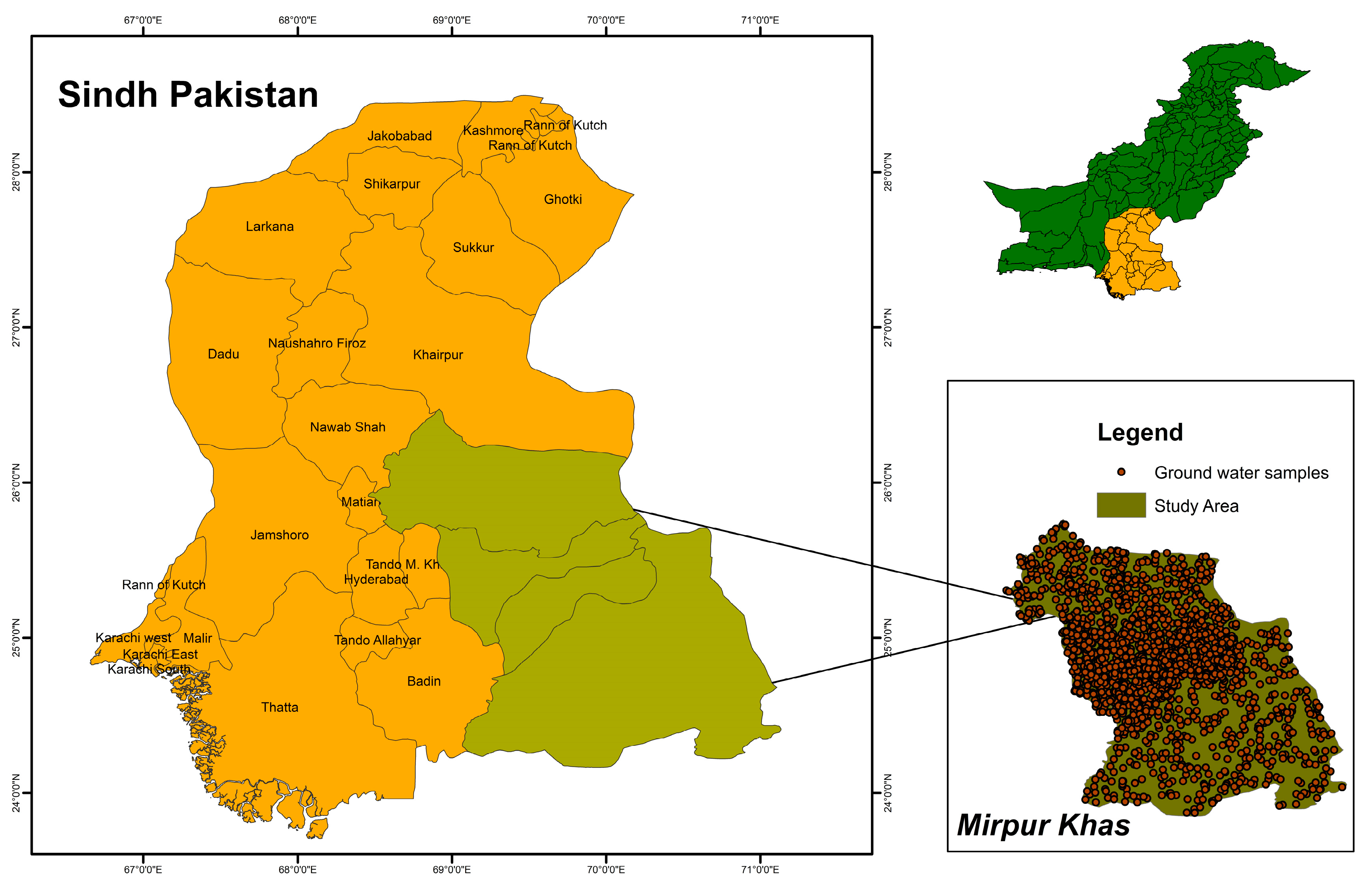
2.1. Study Area
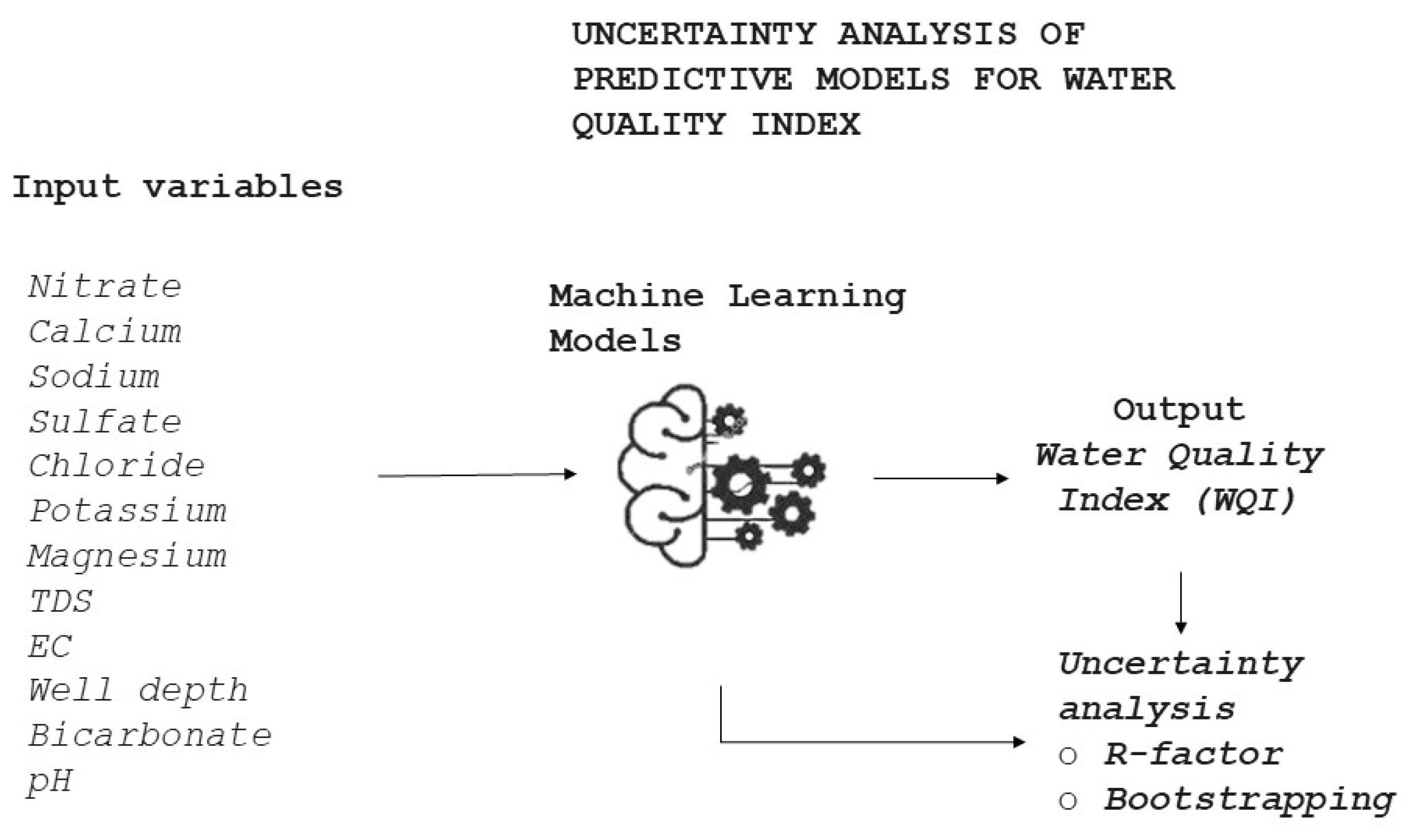
2.2. Methodology
2.3. Uncertainty Analysis
2.3.1. R-Factor
2.3.2. Bootstrapping
2.3.3. Random Forest and Gradient Boosting
2.3.4. Support Vector Machine (SVM) and XGBoost
2.3.5. K-Nearest Neighbors (KNN) and Decision Trees
3. Results
3.1. AUC-Based Performance Evaluation
3.2. Statistical Analysis Using Friedman Test
3.3. Nemenyi Test for Pairwise Comparisons
3.4. Confusion Matrix
4. Discussion
5. Conclusions
Author Contributions
Funding
Data Availability Statement
Conflicts of Interest
References
- Rao, E.P.; Puttanna, K.; Sooryanarayana, K.; Biswas, A.; Arunkumar, J. Assessment of nitrate threat to water quality in India. In The Indian Nitrogen Assessment; Elsevier: Amsterdam, The Netherlands, 2017; pp. 323–333. [Google Scholar]
- Wanke, H.; Nakwafila, A.; Hamutoko, J.; Lohe, C.; Neumbo, F.; Petrus, I.; David, A.; Beukes, H.; Masule, N.; Quinger, M. Hand dug wells in Namibia: An underestimated water source or a threat to human health? Phys. Chem. Earth Parts A/B/C 2014, 76, 104–113. [Google Scholar] [CrossRef]
- Brown, T.C.; Froemke, P. Nationwide assessment of nonpoint source threats to water quality. BioScience 2012, 62, 136–146. [Google Scholar] [CrossRef]
- Lapworth, D.; Boving, T.; Kreamer, D.; Kebede, S.; Smedley, P. Groundwater quality: Global threats, opportunities and realising the potential of groundwater. Sci. Total Environ. 2022, 811, 152471. [Google Scholar] [CrossRef] [PubMed]
- Memon, A.H.; Lund, G.M.; Channa, N.A.; Younis, M.; Ali, S.; Shah, F.B. Analytical Study of Drinking Water Quality Sources of Dighri Sub-division of Sindh, Pakistan. J. Environ. Agric. Sci. 2016, 8, 38–44. [Google Scholar]
- Khan, S.; Aziz, T.; Noor-Ul-Ain, A.K.; Ahmed, I.; Nida, A. Drinking water quality in 13 different districts of Sindh, Pakistan. Health Care Curr. Rev. 2018, 6, 1000235. [Google Scholar]
- Akhan, F.; Siddqui, I.; USMANI, T. of Larkana and Mirpurkhas Districts of Sind. J. Chem. Soc. Pak. Vol. 2006, 28, 131. [Google Scholar]
- Hayder, G.; Kurniawan, I.; Mustafa, H.M. Implementation of machine learning methods for monitoring and predicting water quality parameters. Biointerface Res. Appl. Chem. 2020, 11, 9285–9295. [Google Scholar]
- Avila, R.; Horn, B.; Moriarty, E.; Hodson, R.; Moltchanova, E. Evaluating statistical model performance in water quality prediction. J. Environ. Manag. 2018, 206, 910–919. [Google Scholar] [CrossRef]
- Ashwini, K.; Vedha, J.; Priya, M. Intelligent model for predicting water quality. Int. J. Adv. Res. Ideas Innov. Technol. ISSN 2019, 5, 70–75. [Google Scholar]
- Kalin, L.; Isik, S.; Schoonover, J.E.; Lockaby, B.G. Predicting water quality in unmonitored watersheds using artificial neural networks. J. Environ. Qual. 2010, 39, 1429–1440. [Google Scholar] [CrossRef] [PubMed]
- McGrane, S.J. Impacts of urbanisation on hydrological and water quality dynamics, and urban water management: A review. Hydrol. Sci. J. 2016, 61, 2295–2311. [Google Scholar] [CrossRef]
- Dutt, V.; Sharma, N. Potable water quality assessment of traditionally used springs in a hilly town of Bhaderwah, Jammu and Kashmir, India. Environ. Monit. Assess. 2022, 194, 30. [Google Scholar] [CrossRef]
- Lermontov, A.; Yokoyama, L.; Lermontov, M.; Machado, M.A.S. River quality analysis using fuzzy water quality index: Ribeira do Iguape river watershed, Brazil. Ecol. Indic. 2009, 9, 1188–1197. [Google Scholar] [CrossRef]
- De Pauw, N.; Vanhooren, G. Method for biological quality assessment of watercourses in Belgium. Hydrobiologia 1983, 100, 153–168. [Google Scholar] [CrossRef]
- Zhang, Y.; Guo, F.; Meng, W.; Wang, X.-Q. Water quality assessment and source identification of Daliao river basin using multivariate statistical methods. Environ. Monit. Assess. 2009, 152, 105–121. [Google Scholar] [CrossRef]
- Lenat, D.R. Water quality assessment of streams using a qualitative collection method for benthic macroinvertebrates. J. N. Am. Benthol. Soc. 1988, 7, 222–233. [Google Scholar] [CrossRef]
- Behmel, S.; Damour, M.; Ludwig, R.; Rodriguez, M. Water quality monitoring strategies—A review and future perspectives. Sci. Total Environ. 2016, 571, 1312–1329. [Google Scholar] [CrossRef]
- Hassan, M.M.; Hassan, M.M.; Akter, L.; Rahman, M.M.; Zaman, S.; Hasib, K.M.; Jahan, N.; Smrity, R.N.; Farhana, J.; Raihan, M. Efficient prediction of water quality index (WQI) using machine learning algorithms. Hum.-Centric Intell. Syst. 2021, 1, 86–97. [Google Scholar] [CrossRef]
- Lap, B.Q.; Du Nguyen, H.; Hang, P.T.; Phi, N.Q.; Hoang, V.T.; Linh, P.G.; Hang, B.T.T. Predicting water quality index (WQI) by feature selection and machine learning: A case study of An Kim Hai irrigation system. Ecol. Inform. 2023, 74, 101991. [Google Scholar] [CrossRef]
- Ding, F.; Zhang, W.; Cao, S.; Hao, S.; Chen, L.; Xie, X.; Li, W.; Jiang, M. Optimization of water quality index models using machine learning approaches. Water Res. 2023, 243, 120337. [Google Scholar] [CrossRef] [PubMed]
- Van Rossum, G. Python Programming Language. In Proceedings of the USENIX Annual Technical Conference, Santa Clara, CA, USA, 17–22 June 2007; pp. 1–36. [Google Scholar]
- Saabith, A.S.; Vinothraj, T.; Fareez, M. Popular python libraries and their application domains. Int. J. Adv. Eng. Res. Dev. 2020, 7, 18–26. [Google Scholar]
- Bansal, S.; Ganesan, G. Advanced evaluation methodology for water quality assessment using artificial neural network approach. Water Resour. Manag. 2019, 33, 3127–3141. [Google Scholar] [CrossRef]
- Gevrey, M.; Rimet, F.; Park, Y.S.; Giraudel, J.L.; Ector, L.; Lek, S. Water quality assessment using diatom assemblages and advanced modelling techniques. Freshw. Biol. 2004, 49, 208–220. [Google Scholar] [CrossRef]
- Uddin, M.G.; Olbert, A.I.; Nash, S. Assessment of Water Quality Using Water Quality Index (WQI) Models and Advanced Geostatistical Technique; Civil Engineering Research Association of Ireland (CERAI): Dublin, Ireland, 2020; pp. 594–599. Available online: https://aran.library.nuigalway.ie/bitstream/handle/10379/16427/CERI2020_Uddin_EBK_final.pdf?sequence=1 (accessed on 1 March 2024).
- Mohammadpour, R.; Shaharuddin, S.; Chang, C.K.; Zakaria, N.A.; Ghani, A.A.; Chan, N.W. Prediction of water quality index in constructed wetlands using support vector machine. Environ. Sci. Pollut. Res. 2015, 22, 6208–6219. [Google Scholar] [CrossRef]
- Juna, A.; Umer, M.; Sadiq, S.; Karamti, H.; Eshmawi, A.A.; Mohamed, A.; Ashraf, I. Water quality prediction using KNN imputer and multilayer perceptron. Water 2022, 14, 2592. [Google Scholar] [CrossRef]
- Nasir, N.; Kansal, A.; Alshaltone, O.; Barneih, F.; Sameer, M.; Shanableh, A.; Al-Shamma’a, A. Water quality classification using machine learning algorithms. J. Water Process Eng. 2022, 48, 102920. [Google Scholar] [CrossRef]
- Hussein, E.E.; Jat Baloch, M.Y.; Nigar, A.; Abualkhair, H.F.; Aldawood, F.K.; Tageldin, E. Machine learning algorithms for predicting the water quality index. Water 2023, 15, 3540. [Google Scholar] [CrossRef]
- Khoi, D.N.; Quan, N.T.; Linh, D.Q.; Nhi, P.T.T.; Thuy, N.T.D. Using machine learning models for predicting the water quality index in the La Buong River, Vietnam. Water 2022, 14, 1552. [Google Scholar] [CrossRef]
- Asadollah, S.B.H.S.; Sharafati, A.; Motta, D.; Yaseen, Z.M. River water quality index prediction and uncertainty analysis: A comparative study of machine learning models. J. Environ. Chem. Eng. 2021, 9, 104599. [Google Scholar] [CrossRef]
- Soomro, A.; Mangrio, M.; Bharchoond, Z.; Mari, F.; Pirzada, P.; Lashari, B.; Bhatti, M.; Skogerboe, G. Maintenance Plans for Irrigation Facilities of Pilot Distributaries in Sindh Province, Pakistan. Volume 3—Bareji Distributary, Mirpurkhas District; IWMI: Colombo, Sri Lanka, 1997. [Google Scholar]
- Van der Hoek, W.; Boelee, E.; Konradsen, F. Irrigation, Domestic Water Supply and Human Health; Encyclopedia of Life Support Systems (EOLSS): Paris, France, 2002. [Google Scholar]
- Van der Hoek, W.; Konradsen, F.; Ensink, J.H.; Mudasser, M.; Jensen, P.K. Irrigation water as a source of drinking water: Is safe use possible? Trop. Med. Int. Health 2001, 6, 46–54. [Google Scholar] [CrossRef]
- Akhtar, N.; Syakir Ishak, M.I.; Bhawani, S.A.; Umar, K. Various natural and anthropogenic factors responsible for water quality degradation: A review. Water 2021, 13, 2660. [Google Scholar] [CrossRef]
- Khatri, N.; Tyagi, S. Influences of natural and anthropogenic factors on surface and groundwater quality in rural and urban areas. Front. Life Sci. 2015, 8, 23–39. [Google Scholar] [CrossRef]
- Burri, N.M.; Weatherl, R.; Moeck, C.; Schirmer, M. A review of threats to groundwater quality in the anthropocene. Sci. Total Environ. 2019, 684, 136–154. [Google Scholar] [CrossRef]
- Udhayakumar, R.; Manivannan, P.; Raghu, K.; Vaideki, S. Assessment of physico-chemical characteristics of water in Tamilnadu. Ecotoxicol. Environ. Saf. 2016, 134, 474–477. [Google Scholar] [CrossRef]
- Patil, P.; Sawant, D.; Deshmukh, R. Physico-chemical parameters for testing of water—A review. Int. J. Environ. Sci. 2012, 3, 1194–1207. [Google Scholar]
- Brusseau, M.; Walker, D.; Fitzsimmons, K. Physical-chemical characteristics of water. In Environmental and Pollution Science; Elsevier: Amsterdam, The Netherlands, 2019; pp. 23–45. [Google Scholar]
- Beutler, M.; Wiltshire, K.; Meyer, B.; Moldaenke, C.; Luring, C.; Meyerhofer, M.; Hansen, U. APHA (2005), Standard Methods for the Examination of Water and Wastewater, Washington DC: American Public Health Association. Ahmad, SR, and DM Reynolds (1999), Monitoring of water quality using fluorescence technique: Prospect of on-line process control. Dissolved Oxyg. Dyn. Model. Case Study A Subtrop. Shallow Lake 2014, 217, 95. [Google Scholar]
- Kroll, C.N.; Song, P. Impact of multicollinearity on small sample hydrologic regression models. Water Resour. Res. 2013, 49, 3756–3769. [Google Scholar] [CrossRef]
- Sulaiman, M.S.; Abood, M.M.; Sinnakaudan, S.K.; Shukor, M.R.; You, G.Q.; Chung, X.Z. Assessing and solving multicollinearity in sediment transport prediction models using principal component analysis. ISH J. Hydraul. Eng. 2021, 27, 343–353. [Google Scholar] [CrossRef]
- Iliou, T.; Anagnostopoulos, C.-N.; Nerantzaki, M.; Anastassopoulos, G. A novel machine learning data preprocessing method for enhancing classification algorithms performance. In Proceedings of the 16th International Conference on Engineering Applications of Neural Networks (INNS), Rhodes, Greece, 25–28 September 2015; pp. 1–5. [Google Scholar]
- Werner de Vargas, V.; Schneider Aranda, J.A.; dos Santos Costa, R.; da Silva Pereira, P.R.; Victória Barbosa, J.L. Imbalanced data preprocessing techniques for machine learning: A systematic mapping study. Knowl. Inf. Syst. 2023, 65, 31–57. [Google Scholar] [CrossRef]
- Veček, N.; Črepinšek, M.; Mernik, M. On the influence of the number of algorithms, problems, and independent runs in the comparison of evolutionary algorithms. Appl. Soft Comput. 2017, 54, 23–45. [Google Scholar] [CrossRef]
- Liang, G.; Zhang, C. A comparative study of sampling methods and algorithms for imbalanced time series classification. In Proceedings of the AI 2012: Advances in Artificial Intelligence: 25th Australasian Joint Conference, Sydney, Australia, 4–7 December 2012; pp. 637–648. [Google Scholar]
- Browne, M.W. Cross-validation methods. J. Math. Psychol. 2000, 44, 108–132. [Google Scholar] [CrossRef]
- Daoud, J.I. Multicollinearity and regression analysis. J. Phys. Conf. Ser. 2017, 949, 012009. [Google Scholar] [CrossRef]
- Akram, P.; Solangi, G.S.; Shehzad, F.R.; Ahmed, A. Groundwater Quality Assessment using a Water Quality Index (WQI) in Nine Major Cities of Sindh, Pakistan. Int. J. Res. Environ. Sci. IJRES 2020, 6, 18–26. [Google Scholar]
- Abbas, F.; Zhang, F.; Ismail, M.; Khan, G.; Iqbal, J.; Alrefaei, A.F.; Albeshr, M.F. Optimizing machine learning algorithms for landslide susceptibility mapping along the Karakoram Highway, Gilgit Baltistan, Pakistan: A comparative study of baseline, bayesian, and metaheuristic hyperparameter optimization techniques. Sensors 2023, 23, 6843. [Google Scholar] [CrossRef]
- Wijaya, D.R.; Sarno, R.; Zulaika, E. Information Quality Ratio as a novel metric for mother wavelet selection. Chemom. Intell. Lab. Syst. 2017, 160, 59–71. [Google Scholar] [CrossRef]
- Singhee, A.; Rutenbar, R.A. Why quasi-Monte Carlo is better than Monte Carlo or Latin hypercube sampling for statistical circuit analysis. IEEE Trans. Comput.-Aided Des. Integr. Circuits Syst. 2010, 29, 1763–1776. [Google Scholar] [CrossRef]
- Hoffman, R.N.; Kalnay, E. Lagged average forecasting, an alternative to Monte Carlo forecasting. Tellus A Dyn. Meteorol. Oceanogr. 1983, 35, 100–118. [Google Scholar] [CrossRef]
- Feroz, F.; Hobson, M.P. Multimodal nested sampling: An efficient and robust alternative to Markov Chain Monte Carlo methods for astronomical data analyses. Mon. Not. R. Astron. Soc. 2008, 384, 449–463. [Google Scholar] [CrossRef]
- Noori, R.; Karbassi, A.; Moghaddamnia, A.; Han, D.; Zokaei-Ashtiani, M.; Farokhnia, A.; Gousheh, M.G. Assessment of input variables determination on the SVM model performance using PCA, Gamma test, and forward selection techniques for monthly stream flow prediction. J. Hydrol. 2011, 401, 177–189. [Google Scholar] [CrossRef]
- Pan, M.; Li, C.; Liao, J.; Lei, H.; Pan, C.; Meng, X.; Huang, H. Design and modeling of PEM fuel cell based on different flow fields. Energy 2020, 207, 118331. [Google Scholar] [CrossRef]
- Pirmohamed, M.; Burnside, G.; Eriksson, N.; Jorgensen, A.L.; Toh, C.H.; Nicholson, T.; Kesteven, P.; Christersson, C.; Wahlström, B.; Stafberg, C. A randomized trial of genotype-guided dosing of warfarin. N. Engl. J. Med. 2013, 369, 2294–2303. [Google Scholar] [CrossRef]
- Sharafati, A.; Yasa, R.; Azamathulla, H.M. Assessment of stochastic approaches in prediction of wave-induced pipeline scour depth. J. Pipeline Syst. Eng. Pract. 2018, 9, 04018024. [Google Scholar] [CrossRef]
- Natekin, A.; Knoll, A. Gradient boosting machines, a tutorial. Front. Neurorobot. 2013, 7, 21. [Google Scholar] [CrossRef]
- Boulesteix, A.L.; Janitza, S.; Kruppa, J.; König, I.R. Overview of random forest methodology and practical guidance with emphasis on computational biology and bioinformatics. Wiley Interdiscip. Rev. Data Min. Knowl. Discov. 2012, 2, 493–507. [Google Scholar] [CrossRef]
- Fan, J.; Wang, X.; Wu, L.; Zhou, H.; Zhang, F.; Yu, X.; Lu, X.; Xiang, Y. Comparison of Support Vector Machine and Extreme Gradient Boosting for predicting daily global solar radiation using temperature and precipitation in humid subtropical climates: A case study in China. Energy Convers. Manag. 2018, 164, 102–111. [Google Scholar] [CrossRef]
- Jadhav, S.D.; Channe, H. Comparative study of K-NN, naive Bayes and decision tree classification techniques. Int. J. Sci. Res. IJSR 2016, 5, 1842–1845. [Google Scholar]
- Sheldon, M.R.; Fillyaw, M.J.; Thompson, W.D. The use and interpretation of the Friedman test in the analysis of ordinal-scale data in repeated measures designs. Physiother. Res. Int. 1996, 1, 221–228. [Google Scholar] [CrossRef] [PubMed]
- Pereira, D.G.; Afonso, A.; Medeiros, F.M. Overview of Friedman’s test and post-hoc analysis. Commun. Stat.-Simul. Comput. 2015, 44, 2636–2653. [Google Scholar] [CrossRef]
- Pohlert, T. The pairwise multiple comparison of mean ranks package (PMCMR). R Package 2014, 27, 9. [Google Scholar]
- Garcia, S.; Herrera, F. An Extension on “Statistical Comparisons of Classifiers over Multiple Data Sets” for all Pairwise Comparisons. J. Mach. Learn. Res. 2008, 9, 2677–2694. [Google Scholar]
- Townsend, J.T. Theoretical analysis of an alphabetic confusion matrix. Percept. Psychophys. 1971, 9, 40–50. [Google Scholar] [CrossRef]
- Zeng, D.; Song, Y.; Wang, M.; Lu, Y.; Chen, Z.; Xiao, R. A machine learning approach for predicting the performance of oxygen carriers in chemical looping oxidative coupling of methane. Sustain. Energy Fuels 2023, 7, 3464–3470. [Google Scholar] [CrossRef]
- Tran, H.D.; Li, H. Sound event recognition with probabilistic distance SVMs. IEEE Trans. Audio Speech Lang. Process. 2010, 19, 1556–1568. [Google Scholar] [CrossRef]
- Sun, J.; Yang, Y.; Wang, Y.; Wang, L.; Song, X.; Zhao, X. Survival risk prediction of esophageal cancer based on self-organizing maps clustering and support vector machine ensembles. IEEE Access 2020, 8, 131449–131460. [Google Scholar] [CrossRef]
- Zhang, L.; Zhu, T.; Zhang, H.; Xiong, P.; Zhou, W. Fedrecovery: Differentially private machine unlearning for federated learning frameworks. IEEE Trans. Inf. Forensics Secur. 2023, 18, 4732–4746. [Google Scholar] [CrossRef]
- Wang, W.; Liu, X. Intuitionistic fuzzy information aggregation using Einstein operations. IEEE Trans. Fuzzy Syst. 2012, 20, 923–938. [Google Scholar] [CrossRef]


| Feature | VIF |
|---|---|
| TDS (mg/L) | 4209.78 |
| Sodium (mg/L) | 1137.34 |
| Calcium (mg/L) | 425.13 |
| Magnesium (mg/L) | 380.55 |
| Bicarbonate (mg/L) | 58.74 |
| Sulfate (mg/L) | 39.68 |
| Chloride (mg/L) | 31.69 |
| pH | 20.16 |
| EC (us/cm) | 10.20 |
| Nitrate (NO3-N) (mg/L) | 5.45 |
| Well Depth (m) | 1.70 |
| Potassium (mg/L) | 1.43 |
| Feature | IG |
|---|---|
| Nitrate (NO3-N) (mg/L) | 0.876 |
| Calcium (mg/L) | 0.869 |
| Sodium (mg/L) | 0.869 |
| Sulfate (mg/L) | 0.869 |
| Chloride (mg/L) | 0.869 |
| Potassium (mg/L) | 0.869 |
| Magnesium (mg/L) | 0.869 |
| TDS (mg/L) | 0.816 |
| EC (us/cm) | 0.784 |
| Well Depth (m) | 0.525 |
| Bicarbonate (mg/L) | 0.520 |
| pH | 0.509 |
| Classifier | R-Factor |
|---|---|
| K-Nearest Neighbors | 0.83 |
| Decision Trees | 0.77 |
| Gradient Boosting | 0.83 |
| Random Forest | 0.83 |
| SVM | 0.83 |
| XGBoost | 0.83 |
| Algorithm | AUC |
|---|---|
| Decision Trees (DTs) | 0.77 |
| Random Forest (RF) | 0.95 |
| Gradient Boosting | 0.96 |
| K-Nearest Neighbors (KNN) | 0.84 |
| Support Vector Machine (SVM) | 0.92 |
| XGBoost | 0.95 |
| Test | Value |
|---|---|
| Friedman Test—F-value | 5.0 |
| Friedman Test—p-value | 0.4159 |
| XGB Classifier | Random Forest Classifier | Support Vector Classifier | K-Nearest Neighbors Classifier | Gradient Boosting Classifier | Decision Tree Classifier | |
|---|---|---|---|---|---|---|
| 1 | 1.0 | NaN | NaN | NaN | NaN | NaN |
| 2 | NaN | 1.0 | NaN | NaN | NaN | NaN |
| 3 | NaN | NaN | 1.0 | NaN | NaN | NaN |
| 4 | NaN | NaN | NaN | 1.0 | NaN | NaN |
| 5 | NaN | NaN | NaN | NaN | 1.0 | NaN |
| 6 | NaN | NaN | NaN | NaN | NaN | 1.0 |
| True\Predicted | Class 1 | Class 2 | Class 3 | Class 4 | Class 5 |
|---|---|---|---|---|---|
| Class 1 | 2 (TP) | 3 (FN) | 0 | 0 | 0 |
| Class 2 | 0 | 3 (TP) | 0 | 1 (FP) | 0 |
| Class 3 | 0 | 3 (FP) | 1 (TP) | 2 (FP) | 1 (TN) |
| Class 4 | 0 | 2 (FP) | 0 | 1 (TP) | 1 (TN) |
| Class 5 | 0 | 0 | 0 | 2 (FP) | 62 (TP) |
| True\Predicted | Class 1 | Class 2 | Class 3 | Class 4 | Class 5 |
|---|---|---|---|---|---|
| Class 1 | 4 (TP) | 1 (FN) | 0 | 0 | 0 |
| Class 2 | 2 (FP) | 1 (TP) | 0 | 0 | 1 (FN) |
| Class 3 | 0 | 1 (FP) | 1 (TP) | 2 (FP) | 3 (TN) |
| Class 4 | 0 | 1 (FP) | 0 | 0 | 3 (TN) |
| Class 5 | 0 | 0 | 0 | 0 | 64 (TP) |
| True\Predicted | Class 1 | Class 2 | Class 3 | Class 4 | Class 5 |
|---|---|---|---|---|---|
| Class 1 | 4 (TP) | 1 (FN) | 0 | 0 | 0 |
| Class 2 | 2 (FP) | 1 (TP) | 0 | 0 | 1 (FN) |
| Class 3 | 1 (FP) | 0 | 0 | 0 | 6 (FN) |
| Class 4 | 0 | 0 | 0 | 0 | 4 (FN) |
| Class 5 | 0 | 0 | 0 | 0 | 64 (TP) |
| True\Predicted | Class 1 | Class 2 | Class 3 | Class 4 | Class 5 |
|---|---|---|---|---|---|
| Class 1 | 3 (TP) | 2 (FN) | 0 | 0 | 0 |
| Class 2 | 3 (TP) | 0 | 0 | 0 | 1 (FN) |
| Class 3 | 0 | 2 (FP) | 1 (TP) | 1 (FP) | 3 (TN) |
| Class 4 | 0 | 0 | 0 | 0 | 4 (TN) |
| Class 5 | 0 | 1 (FP) | 1 (TP) | 2 (FP) | 60 (TP) |
| True\Predicted | Class 1 | Class 2 | Class 3 | Class 4 | Class 5 |
|---|---|---|---|---|---|
| Class 1 | 4 (TP) | 1 (FN) | 0 | 0 | 0 |
| Class 2 | 2 (FP) | 1 (TP) | 0 | 1 (FP) | 0 |
| Class 3 | 0 | 2 (FP) | 2 (TP) | 2 (FP) | 1 (TN) |
| Class 4 | 0 | 2 (FP) | 0 | 1 (TP) | 1 (TN) |
| Class 5 | 0 | 0 | 0 | 0 | 64 (TP) |
| True\Predicted | Class 1 | Class 2 | Class 3 | Class 4 | Class 5 |
|---|---|---|---|---|---|
| Class 1 | 4 (TP) | 1 (FN) | 0 | 0 | 0 |
| Class 2 | 2 (FP) | 2 (TP) | 0 | 0 | 0 |
| Class 3 | 0 | 1 (FP) | 3 (TP) | 2 (FP) | 1 (TN) |
| Class 4 | 0 | 1 (FP) | 1 (FP) | 1 (TP) | 1 (TN) |
| Class 5 | 0 | 1 (FP) | 0 (FP) | 2 (FP) | 61 (TP) |
| Classes | WQI Range | Water Quality |
|---|---|---|
| Class 1 | 0–25 | Excellent water quality |
| Class 2 | 26–50 | Good water quality |
| Class 3 | 51–75 | Fair water quality |
| Class 4 | 76–100 | Poor water quality |
| Class 5 | Above 100 | Very poor to unacceptable water quality |
| TDS | EC | Well Depth | pH | Sulfate | Chloride | Sodium | Potassium | Magnesium | Calcium | Bicarbonate | Nitrate (NO3-N) | Rescaled_WQI | Model Predicted_WQI_Code |
|---|---|---|---|---|---|---|---|---|---|---|---|---|---|
| 281 | 2892 | 24 | 8.5 | 17.12571 | 30.90157 | 17.18087 | 0.380653 | 6.112794 | 57.36129 | 82.53007 | 23.6361 | 134 | 5 |
| 285 | 2455 | 33 | 7.99 | 10.50744 | 25.27189 | 15.79175 | 0.880966 | 10.69318 | 73.59643 | 233.2372 | 5.283148 | 104 | 5 |
| 293 | 1266 | 47.1 | 7.39 | 15.33482 | 14.97501 | 35.97985 | 1.158209 | 14.11058 | 54.82109 | 275.1002 | 3.197757 | 6 | 1 |
| 302 | 2111 | 25 | 7.56 | 30.84742 | 22.94148 | 12.19949 | 1.193796 | 12.96383 | 78.09345 | 358.8264 | 5.686334 | 80 | 4 |
| 310 | 2000 | 19 | 8.37 | 67.98364 | 36.64451 | 20.84443 | 2.2859 | 15.15061 | 69.56399 | 358.8264 | 0.239171 | 76 | 4 |
| 370 | 1712 | 33 | 7.37 | 50.69821 | 23.40693 | 9.955348 | 0.890684 | 9.830066 | 103.6547 | 358.8264 | 10.54824 | 43 | 2 |
| 405 | 1122 | 300 | 8.21 | 768.8918 | 27.44628 | 15.49567 | 1.111356 | 14.22923 | 98.52735 | 358.8264 | 2.862759 | 66 | 3 |
| 406 | 1242 | 60 | 6.91 | 54.48075 | 152.4355 | 14.49937 | 1.267128 | 16.98422 | 106.119 | 358.8264 | 27.40252 | 26 | 2 |
| 406 | 1242 | 40 | 6.91 | 55.73943 | 30.83817 | 8.220457 | 1.118785 | 21.9048 | 105.0737 | 358.8264 | 7.057716 | 17 | 1 |
| 409 | 1829 | 101 | 10.94 | 59.5349 | 12.51032 | 5.80349 | 0.708562 | 10.05297 | 125.124 | 358.8264 | 8.928545 | 67 | 3 |
| 479 | 1972 | 265 | 9.18 | 54.17818 | 62.93912 | 23.93549 | 0.597271 | 21.97534 | 119.45 | 358.8264 | 3.133473 | 98 | 4 |
Disclaimer/Publisher’s Note: The statements, opinions and data contained in all publications are solely those of the individual author(s) and contributor(s) and not of MDPI and/or the editor(s). MDPI and/or the editor(s) disclaim responsibility for any injury to people or property resulting from any ideas, methods, instructions or products referred to in the content. |
© 2024 by the authors. Licensee MDPI, Basel, Switzerland. This article is an open access article distributed under the terms and conditions of the Creative Commons Attribution (CC BY) license (https://creativecommons.org/licenses/by/4.0/).
Share and Cite
Abbas, F.; Cai, Z.; Shoaib, M.; Iqbal, J.; Ismail, M.; Arifullah; Alrefaei, A.F.; Albeshr, M.F. Machine Learning Models for Water Quality Prediction: A Comprehensive Analysis and Uncertainty Assessment in Mirpurkhas, Sindh, Pakistan. Water 2024, 16, 941. https://doi.org/10.3390/w16070941
Abbas F, Cai Z, Shoaib M, Iqbal J, Ismail M, Arifullah, Alrefaei AF, Albeshr MF. Machine Learning Models for Water Quality Prediction: A Comprehensive Analysis and Uncertainty Assessment in Mirpurkhas, Sindh, Pakistan. Water. 2024; 16(7):941. https://doi.org/10.3390/w16070941
Chicago/Turabian StyleAbbas, Farkhanda, Zhihua Cai, Muhammad Shoaib, Javed Iqbal, Muhammad Ismail, Arifullah, Abdulwahed Fahad Alrefaei, and Mohammed Fahad Albeshr. 2024. "Machine Learning Models for Water Quality Prediction: A Comprehensive Analysis and Uncertainty Assessment in Mirpurkhas, Sindh, Pakistan" Water 16, no. 7: 941. https://doi.org/10.3390/w16070941