Numerical Simulation of Geophysical Models to Detect Mining Tailings’ Leachates within Tailing Storage Facilities

Abstract

The effective detection and monitoring of mining tailings’ leachates (MTLs) plays a pivotal role in environmental protection and remediation efforts. Electrical resistivity tomography (ERT) is a non-invasive technique widely employed for mapping subsurface contaminant plumes. However, the efficacy of ERT depends on selecting the optimal electrode array for each specific case. This study addresses this challenge by conducting a comprehensive review of published case studies utilizing ERT to characterize mining tailings. Through numerical simulations, we compare the imaging capabilities of commonly used electrode configurations, six ERT arrays, aiming to identify the optimal array for MTLs’ detection and monitoring. In addition, field surveys employing ERT were conducted at the El Mochito mine tailings site to detect zones saturated with leachates within the tailing storage facilities (TSFs). The findings indicate that the “Wenner-Schlumberger” array exhibits superior data resolution for MTL detection. However, the choice of the optimal electrode array is contingent on factors such as survey location, geological considerations, research objectives, data processing time and cost, and logistical constraints. This study serves as a practical guide for selecting the most effective electrode array in the context of pollutant penetration from mining tailings, employing the ERT technique. Furthermore, it contributes valuable insights into characterizing zones saturated with mining tailing leachates within the TSFs, providing a solid foundation for informed environmental management and remediation strategies.

1. Introduction

Mining tailings are the residual materials remaining following the extraction of valuable minerals from ores. These tailings usually contain toxic chemicals such as arsenic, lead, and mercury, which pose a significant environmental threat if not managed properly [1]. Mining tailings can contaminate soil, water, and air, leading to health hazards for humans and wildlife. The management and disposal of mining tailings are essential to prevent their negative impact on the environment [2,3]. Some of the strategies for managing mining tailings include the construction of tailing dams, the backfilling of mined-out areas, and reprocessing to extract any remaining valuable minerals [4,5]. Despite these efforts, mining tailings remain a significant challenge for the mining industry, as the tailings produced can accumulate for decades or even centuries, with the potential to cause harm to the environment and communities surrounding the mine sites [6].

Geophysical techniques are extensively employed for the monitoring of groundwater contamination, which can arise from diverse sources, including hydrocarbon contamination [7,8], landfills [9,10], saline water intrusions [11,12], and mine tailings [13,14]. These techniques are cost-effective, repeatable, rapid, and non-destructive during data acquisition. Moreover, they provide an informative image of the subsurface petrophysical conditions. These geophysical surveying methods involve the use of the physical and petrophysical properties of the earth to identify the presence and movement of fluids within the ground [15]. The presence of hydrocarbon contaminants stimulates biological and chemical activity, resulting in bio physicochemical changes induced in the subsurface during the reaction of contaminants [16]. The increase in reactions in the surfaces of the substrate and between pore openings in rocks and sediments can induce physical changes in the porous material itself [17]. These reactions result in the production of acids which are responsible for the leaching of the surrounding soil matrix causing an increase in the ionic strength of the pore water. Hence, the dissolution of minerals results in the etching of the grains of the soil matrix [18]. These changes may cause an increase in the bulk electrical conductivity of contaminated soil that is detectable by geophysical methods such as Electrical Resistivity Tomography (ERT) and Ground-Penetrating Radar (GPR) [16,19,20]. These techniques play a crucial role in assessing and understanding the extent and nature of groundwater contamination, enabling effective mitigation strategies and resource management [21,22]. However, choosing the optimal geophysical method that meets the purpose of a project sometimes is challenging and may dictate the success or failure of the subsurface imaging [23,24].

The ERT method has been widely applied in groundwater, mining, environmental, and civil engineering investigations [25,26]. Mineral grains in the subsurface constitute the primary component of nonconductive soil and rock fragments [27,28]. However, in contaminated areas like mining sites, the presence of conductive metallic ores leads to variations in conductivity, creating anomalous zones [29]. As a result, the resistivity of soil and rock fragments can be readily differentiated from conductive zones. Other factors that may affect the resistivity include water in the pore spaces, water salinity, permeability, and porosity [30]. Resistivity measurements can detect anomalies in the subsurface and hence provide an image of the subsurface conditions [31]. Recently, there have been significant advances in automated ERT data acquisition approaches as well as 2D and 3D inversion software [32,33,34]. Thus, ERT has become a more attractive exploration method and a proven non-invasive and cost-effective technique. Many authors have demonstrated the conceivability to obtain accurate resistivity data of the subsurface structure using 2D/3D ERT inversion models [35,36,37,38,39,40,41].

As ERT is very sensitive to electrode array types [42], choosing the right array for each case study can have a substantial impact on the produced image [43,44]. Various numerical, experimental, and field studies have been conducted to compare different ERT electrode arrays for near surface geophysical settings and structures [45,46,47,48,49,50,51,52,53,54]. To our knowledge, there has not been a comprehensive comparison of ERT electrode arrays for mining tailings’ leachates (MTLs). Most of the previous work on MTLs using ERT employed a single electrode array without justification for why this array was employed. Therefore, this study aims to determine the appropriate electrode array that could be used to detect and monitor MTL. In this study, “leachate” pertains to the fluid that accumulates within tailing storage facilities (TSFs) subsequent to leaching through the tailing materials. To achieve this goal, a review of the published case studies in the literature that applied ERT to characterize mining tailings was performed to identify the most commonly used electrode array for such applications. Subsequently, a numerical investigation was conducted to evaluate the imaging capability of the commonly used electrode configurations. This evaluation was performed on a synthetic mining tailing backfilling model. A robust inversion approach was utilized to compare the configurations for 2D ERT, because it is a common inversion scheme for such projects. The following factors were evaluated for each electrode array: the imaging resolution, the depth of investigation (DOI), the data density, and the sensitivity to noise. Additionally, field surveys were conducted at the El Mochito mine tailings site to detect zones saturated with leachate within the tailing storage facilities (TSFs). This methodology is expected to help in selecting the most appropriate electrode array for mapping the MTL.

2. Literature Review

The use of ERT in characterizing mining tailings has become increasingly popular due to their accuracy and cost-effectiveness. In the section below, a review of published case studies that employed ERT to characterize mining tailings with emphasis on identifying the most commonly used electrode array for detecting MTLs within TSFs was conducted. Several criteria were considered while reviewing the published literature, including the following:

(1)

Research focus: choosing the published literature that is closely aligned with the research focus and objectives of this study;

(2)

Relevance: selecting articles that directly address similar or related research questions allows the authors to build upon existing knowledge and establish a coherent framework for their study;

(3)

Methodological compatibility: limiting the selected literature that uses the same electrode arrays and employs a similar or complementary methodologies

(4)

Limitations and scope: Because of limitations on space and the scope of the study, it is not feasible to include all the articles available on a particular topic. Thus, the authors had to make strategic choices to include representative studies that adequately cover the range of relevant perspectives and findings.

The Wenner-Schlumberger (WSC) array was successfully used during a 2D-ERT survey to characterize the environmental hazard of lead and zinc leaching of mine tailings at Frongoch Mine, Ceredigion, UK [55]. Another study was conducted in the Sierra Minera region, Spain, and employed the WSC array combined with soil chemical analyses. Their study helped in mapping the mine-tailing ponds [38]. Similarly, the WSC array was used to identify acid waste drainage from Zn-Pb post-flotation tailing ponds in Olkusz, Poland [14]. The WSC array was also used in the characterization of tailing dams [56], in the evaluation of tailing ponds in Linares, Southern Spain [57]. Meanwhile, the dipole–dipole array was used to assess waste materials in a mining tailing pond in El Gorguel, Spain [58]. ERT was employed to diagnose alteration channel penetration in uranium waste in Osamu Utsumi, Brazil, using the Schlumberger array [59]. The Schlumberger array was used for investigations and evaluation of environmental pollution in a mine tailings area in Komsomolsk, Russia [60]. Moreover, the most suitable spots for mine waste disposal were identified using the Wenner array [35]. Also, the Wenner array was utilized for the assessment of mine wastes in Regoufe, Portugal [61]. Copper mine tailings in Rio Tinto, Spain, were characterized utilizing the Wenner array [62], while the same array was used for undrained oil sands’ tailing ponds in Alberta, Canada [30]. For the characterization of water contamination due to metal mine waste in EsgairMwyn, Ceredigion, a Wenner-α electrode array was used [63]. WSC was employed to characterize abandoned sulfide mine-waste ponds in Iberian, SW Spain [64], and the same array was used for the assessment of the environmental threat of reclaimed mining tailing ponds [65]. The Schlumberger array was utilized for the delineation of subsurface structures in U-tailings in Jaduguda, India [66].

Table 1. A summary of some case studies that applied ERT to characterize mining tailings.

Array	Survey Type	Ore	Mine	Country	Ref.
Wenner-Schlumberger	2D	Lead (Pb) and Zinc (Zn)	Frongoch	UK	[36]
Wenner-Schlumberger	2D/3D	Cadmium (Cd), Copper (Cu), Pb and Zn	Sierra Minera	Spain	[23]
Wenner- Schlumberger	2D	Zn-Pb	Olkusz	Poland	[14]
Wenner–Schlumberger	2D	Zn-Pb	Federico	Spain	[56]
Wenner-Schlumberger	2D	Pb–Ag	Linares	Spain	[57]
Wenner-Schlumberger	2D	Cu–Zn–Pb	Iberian	Spain	[64]
Wenner–Schlumberger	2D	Pb-Cd- Zn	Cordillera Bética	Spain	[65]
Schlumberger	1D/2D	Uranium	Jaduguda	India	[66]
Schlumberger	2D/3D	Uranium	Osamu Utsumi	Brazil	[59]
Schlumberger	2D	Gold	Komsomolsk	Russia	[60]
Wenner	2D	Tungsten	Regoufe	Portugal	[59]
Wenner	2D/3D	Cu	Peña de Hierro	Spain	[62]
Wenner	2D	Oil	Fort McMurray	Canada	[30]
Wenner	2D	Zn-Pb	EsgairMwyn	Ceredigion	[63]
Wenner	2D	Iron	Mount Gibson	Australia	[67]
Wenner	2D	Ag-Pb- Zn	El Mochito	Honduras	[35]
Dipole–dipole	2D	Ni-Cd- Fe	Cartagena-La Union	Spain	[18]

summarizes some of the case studies where ERT was utilized to characterize mining tailings.

3. Methodology

3.1. ERT Technique and Data Collection

ERT method uses the measurement of electrical resistivity to produce images of subsurface structures. The principle of ERT is based on the fact that different materials have different electrical resistivities. Through injecting electrical currents into the ground through two current electrodes (A, B) and tracking the potential difference between two potential electrodes (M, N), the electrical resistivity distribution can be mapped within the subsurface. We make the assumption of subsurface homogeneity and isotropy when calculating apparent resistivity values. However, it is important to note that the subsurface is not truly homogeneous and isotropic.

The datasets collected from these measurements, as shown in Figure 1, are then used to create an image of the subsurface by solving an inverse problem. The inverse problem involves finding the electrical resistivity distribution that best fits the observed data. This is achieved by using a mathematical algorithm that takes into account the geoelectrical properties of the subsurface materials as well as the geometry of the electrode array used in the measurements [68]. The inversion process is the central operation in geophysics, akin to fitting a puzzle in reverse. Instead of predicting measurements based on a model (forward modeling), inversion adjusts model parameters iteratively until calculated measurements closely match observed ones. This involves tweaking parameters, such as material distributions underground, to minimize differences between observed and calculated measurements. Once convergence is reached, the final model represents the possible model of the subsurface distribution based on the measured apparent resistivities, revealing helpful information about geological or hydrogeological features. Some common electrode configurations and their geometric factors (k) are shown in Figure 2 and

Table 2. Geometric factors for electrode configurations illustrated in Figure 2.

Array Type	Geometric Factor (K)
Wenner-α	2πa
Wenner-β	6πa
Wenner-γ	3πa
Dipole–dipole	πna(1 + n)(1 + 2n)
Schlumberger	πb(b + a)/a
Wenner-Schlumberger	πna(1 + n)

, respectively.

3.2. Synthetic ERT Model for MTL

A synthetic model is a simulated representation of a mining tailing’s backfilling scenario. In the context of ERT, a synthetic model for MTL has been created to simulate the electrical resistivity of the subsurface materials. The purpose of this model is to numerically examine the capability of six different electrode arrays, shown in Figure 2, in imaging the synthetic MTL model. Three different geoelectric layers were designed, as shown in Figure 3. The top layer has a thickness of 2.5 m with a relatively high resistivity (80 Ωm), indicating a dry tailing’s region. The second layer shows a moderate resistivity value (40 Ωm) and has a thickness of 7.5 m, representing a percolation/leaching (semi-saturated tailings) region. The third layer has a dramatically low resistivity (15 Ωm) and represents the saturated region. This layer indicates active leaching and the presence of conductive materials.

In general, rectangular or square elements are the most commonly used shapes in ERT as they are easy to implement, and they offer good accuracy for most practical applications [70]. However, non-rectangular or non-square elements such as triangles or hexagons may be a better fit for subsurface regions with irregular shapes or complex geometries. These shapes can provide a better resolution of subsurface features and hence reduce the number of computational resources needed to discretize the subsurface region [71,72].

This study compared the six electrode configurations used in the literature to characterize mining tailings, as mentioned earlier. The minimum electrode spacing is 2 m and the total number of electrodes is 50 for each configuration.

Several numerical modelling software packages are available for simulating electrical measurements in ERT. RES2DMOD is one of the most common software packages for such cases [45]. The forward-modelling algorithm which we applied via RES2DMOD is based on the finite element method, which solves the forward problem of ERT by discretizing the subsurface into a grid and calculating the resistivity values at each grid node.

Noise and errors were added to the simulated measurements to mimic the real subsurface and make them more realistic. This can be achieved by randomly perturbing the simulated measurements or by adding noise that follows a specific distribution (e.g., Gaussian). The average Gaussian noise value that can be added to an ERT model depends on several factors, including the signal-to-noise ratio (SNR) of the original data, the complexity of the subsurface structure, the purpose of the model, and the desired level of accuracy and precision. Also, the amount of noise added was based on expected noise levels in actual field measurements and should be considered when interpreting the results, which generally range from 5% to 20% [72]. Based on the noise value of the real-world case, 15% was added to the synthetic data to identify the strengths and weaknesses of different electrode configurations and provide insights into how to optimize the design of ERT surveys for MTL applications.

The inversion software used here is RES2DINV (V4.08, Geotomo Software, Penang, Malaysia), a software package for inverting ERT data to estimate the subsurface resistivity distribution. The optimization inversion algorithm by RES2DINV is based on the robust least squares method [73,74], which compares the calculated and measured data at each electrode position. The inversion process was repeated until a convergence criterion was met, such as a minimum change in the misfit function or a maximum number of iterations.

The accuracy of the synthetic model was evaluated by comparing the inverted electrical resistivity values to the true values assigned in step 2. This was achieved using various metrics, such as the root mean square (RMS) error or correlation coefficient. The details are explained in the next section.

3.3. Real Case of ERT Field Surveys for MTL

Figure 4a displays the detailed location of the El Mochito mine site. The site is situated in the northwestern region of Honduras, proximate to Las Vegas [35]. It is positioned approximately 88 km to the southwest of San Pedro Sula and 220 km to the northwest of the capital city, Tegucigalpa. The survey area encompasses a range of latitude and longitude coordinates, specifically 14.86° N, −88.07° W to 14.87° N, −88.06° W. Additionally, the coordinate reference system employed is EPSG:4267—NAD27.

The El Mochito mining facility comprises an underground operation extracting lead, zinc, and silver ores, with a concentrator that separates zinc and lead concentrates. Ore processing involves a traditional sulfide flotation system, handling an average of 2250 tons per day (t/d), leading to the generation of substantial waste, amounting to 300 t/d, in the flotation plants. Liquid tailings, produced after separating solids, are transported via a 4.5 km pipeline to TSFs [29]. The El Mochito mine has numerous TSFs, enabling continuous mining activities. This study was conducted on the El Bosque dump, the earliest TSF, containing approximately 5 million tons of old mining tailings. Closed officially in 2018, the dump’s surface has undergone natural re-vegetation. Figure 4b,c depicts the spatial distribution of profile positions and the extent of electrode spacing along the tailing. The ERT data was systematically acquired along multiple surface profiles with a uniform interval of 40 m, while the electrodes were separated by a distance of 2.3 m. A survey employing the EarthProbe high resolution DCIP system, as demonstrated in Figure 5, was conducted for ERT.

4. Results

4.1. Results of the Synthetic ERT Model for MTL

The efficiency and resolution of these six electrode configurations for detecting MTL using the ERT survey were compared through numerical simulations, and 2D resistivity inversion results are shown in Figure 6. The comparison of these six electrode configurations for detecting MTL using ERT was based on various factors, including data resolution, depth of investigation (DOI), data density, and sensitivity to noise, as listed in

Table 3. Comparing the results of the six electrode configurations for detecting MTL using the ERT survey.

Array	Number of Data Points	Average Sensitivity		DOI	Resolution	Abs. Errors, %	RMS, %
W-α	335	2.831	Moderate	Shallow	Moderate	0.78	0.97
W-β	335	2.847	Moderate	Shallow	Moderate	0.81	1.04
W-γ	335	3.398	Moderate	Shallow	Moderate	0.7	0.87
DD	425	6.241	High	Moderate	High	0.87	1.1
Sch	520	4.231	High	Moderate	High	0.76	0.98
WSC	640	4.440	High	Moderate/Deep	High	0.79	1

. The results of the 2D inversion show that each electrode configuration has its advantages and disadvantages.

For the Wenner Alpha (W-α), Beta (W-β), and Gamma (W-γ) arrays, a total of 335 data points were collected using each array. The sections images map ~11, ~9, and ~13 m below surface, respectively. An average sensitivity of three and moderate resolution is observed for the three arrays. Three layers were mapped using each array. However, thicknesses vary for each array.

The dipole–dipole (DD) array measured more data points compared to Wenner arrays with a total 425 data points; however, the maximum model depth is ~6 m which is the least compared to all other arrays. This array mapped three layers and provided more details about the MTL changes in the subsurface.

The Schlumberger (Sch) array measured more data points compared to both Wenner and DD arrays with a total of 520 data points. The maximum model depth is ~13 m, and the array mapped three layers.

The Wenner-Schlumberger (WSC) array measured the highest number of data points compared to all other arrays with a total of 640 data points. The maximum model depth is ~18 m which is the deepest compared to all other arrays.

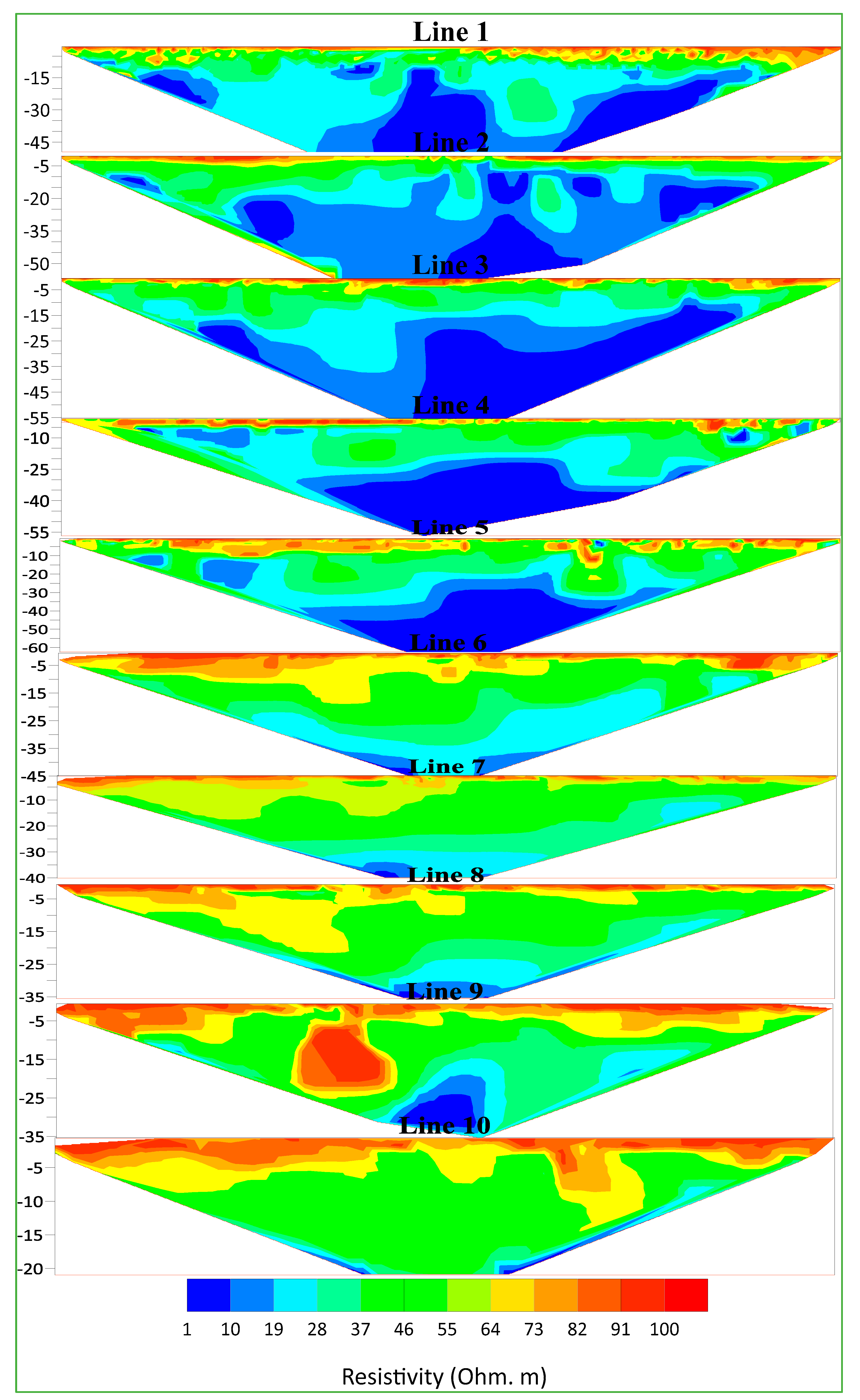
4.2. Results of the Real Case

The ERT field survey was conducted in this study to confirm the results of the synthetic ERT model for MTL. The data acquisition was conducted along various 2D parallel profiles using the W-α array. These profiles covered varying lengths, ranging from 104 to 363 m, allowing for the mapping of subsurface conditions to a maximum depth of approximately 60 m. The inverted ERT data revealed consistent patterns of decreasing resistivity with increasing depth across all profiles; some of these profiles/lines are illustrated in Figure 7, as an example, the results of all these profiles can be found in Appendix A, Figure A1.

Figure 8 illustrates the RMS and absolute errors of the inversion results, considering the inclusion of data-point outliers. Subfigure (a) presents a histogram, providing a visual representation of the percentage of total data points against the apparent resistivity percentage errors. This histogram allows for an overview of the distribution of errors throughout the dataset. The tallest bar in the bar chart represents the smallest error, and as the error increases, the height of the bars decreases. This indicates the quality of the measured data points, as negative resistivity values, spikes, and erroneous data points have been removed before conducting the inversion to generate an accurate inversion model. In subfigure (b), a scatter plot visualizes the misfit results by showcasing the disparity between the calculated and measured apparent resistivity values. The scatter plot offers a detailed examination of individual data points, aiding in the identification of outliers and contributing to a comprehensive understanding of the inversion accuracy and reliability. Outliers account for less than 2% of the data, and the errors are as follows: the L1-norm data misfit is 9.212%, and the L2-norm data misfit is 18.55%.

5. Discussion

The results of the modeling investigations indicate that the Wenner Alpha (W-α) array provides a relatively decent data resolution (data density) by measuring the apparent resistivity at various electrode spacings (i.e., a moderate data density compared to other electrode arrays). The top layer, representing a dry tailing region, has a thickness that is almost the same as the synthetic model (2.5 m) with a small difference in resistivity value. Similarly, the second layer represents a percolation/leaching (semi-saturated tailings) region of which the boundaries are well resolved in the inverse resistivity model. However, the third layer, which represents the saturated tailings region, has a relatively low data resolution due to the wide electrode spacing. The maximum model depth of this array has a moderate depth of investigation because the depth to which the Wenner-alpha array can investigate the subsurface is much smaller than the maximum AB separation (<AB/6). This can also be seen in Figure 7, where the maximum AB separation of ~400 m corresponds to a maximum depth of ~56 m. Thus, for deeper investigations, a wider electrode spacing is required, which results in data resolution attenuation. Additionally, the data density of the W-α array is relatively low as it requires a relatively large number of electrodes. For sensitivity, the W-α array showed a good sensitivity to resistivity changes at shallower depths, which decreased at greater depths due to current dispersion as it travels deeper into the ground.

The Wenner Beta (W-β) array is a modification of the W-α with a shorter current electrode spacing. Despite the shorter electrode spacing, the W-β array produces a data resolution for the first layer nearly like the W-α array. However, for the other layers, the resolution is lower than that of the W-α array since the DOI of the W-β array is relatively shallow. The W-β array has the same data density as the Wenner array since both use four electrodes. Nevertheless, the W-β array offers a higher sensitivity to subsurface resistivity changes than the W-α array. This increased sensitivity is due to the short electrode spacing, which allows for a greater portion of the subsurface to be investigated, resulting in higher sensitivity to subsurface resistivity changes, especially in shallow applications.

The Wenner Gamma (W-γ) array is another modification of the W-α, where the current and potential electrodes are placed in an alternative order. This means that the electrode spacing is twice that of the W-α electrode spacing. The W-γ array provides a similar data resolution to the W-α, with the electrode spacing being the primary factor affecting data resolution. Smaller electrode spacings result in higher data resolution. The DOI of the W-γ array is better than the W-α, as the current is focused between the outermost electrodes, resulting in deeper penetration. While the data density is the same as the W-α, the sensitivity of the W-γ array is like the Wenner array. However, the higher DOI may result in lower sensitivity at shallower depths.

The dipole–dipole (DD) array is a commonly used configuration for ERT surveys. This array provides good data resolution, as the spacing between the electrodes can be adjusted to optimize data resolution for a particular target depth. The array provides a relatively high data density compared to Wenner arrays, as multiple measurements must be taken at each electrode location. However, this can increase the time and cost of the survey. The DD array is sensitive to both lateral and vertical changes in resistivity, making it a good choice for investigating complex subsurface structures.

The Schlumberger (Sch) array is a commonly used electrode configuration in ERT surveys for characterizing mine tailing dumps. It provides a relatively high data resolution compared to Wenner and DD arrays due to its sensitivity, which is important for detecting small-scale features in the subsurface. The Sch array gives the DOI better than Wenner arrays and can be adjusted by changing the electrode spacing, making it suitable for studying shallow subsurface layers. Additionally, the data density is higher also than that of the Wenner and DD arrays and can be controlled by adjusting the number of electrode measurements, allowing for higher-resolution data in areas of interest. The Sch array is also sensitive to changes in subsurface resistivity, making it useful for detecting subtle variations in the MTL subsurface. The Schlumberger array produced high-quality data with relatively low RMS errors.

The Wenner-Schlumberger (WSC) array is a modification of the Wenner array in which the current electrodes are kept at the same spacing, but the potential electrodes are spaced closer together to increase the sensitivity of the method. The WSC array provides a higher data resolution compared to Wenner and DD arrays due to the increased sensitivity achieved by spacing the potential electrodes closer together. This allows for a better delineation of near-surface features. Moreover, the DOI of the WSC array is higher compared to other arrays such as Wenner, and the data density of the WSC array is higher also than that of the Wenner and DD arrays. Additionally, the increased sensitivity of the WSC array results in a higher-resolution dataset due to the closer spacing of the potential electrodes. This allows for a better delineation of near-surface features and can help to identify subtle changes in subsurface MTLs. Therefore, the WSC array is useful in situations where a high resolution is required at shallow depths, making it a popular choice for environmental and engineering applications. The WSC array, while effective, does come with certain drawbacks. It requires a larger surface area for cable deployment due to the substantial distance between current electrodes. Consequently, surveying expansive areas for MTL plumes can be cumbersome, particularly in access-limited regions. Moreover, the slower acquisition of the WSC array can be time-consuming, which may pose challenges for the dense data collection often required for precise MTL plume delineation.

In addition to the results and analyses obtained from synthetic modeling MTL data, we conducted a field survey of an old mining-tailing pond in Honduras to validate these findings. The inversion results of the field survey are depicted in Figure 7. It is noteworthy that the survey utilized the W-α array for practical reasons, such as the ease and speed of use, as well as calculations. Moreover, this array is widely employed in previous studies for similar applications, as indicated in Table 2. Additionally, the choice aligns with the principle that obtaining satisfactory results with a less efficient array suggests better outcomes with a more efficient one.

Upon the analysis and interpretation of these resistivity profiles in Figure 7, a consistent and distinguishable layering pattern became apparent across all surveyed profiles which is practically consistent with the results of the synthetic modeling for the MTL. The profiles reveal the presence of three geoelectric layers, each with varying thickness and depth. This observation is summarized in

Table 4. A summary of the description geoelectric profiles.

Sequence	Resistivity (Ωm)	Thickness (m)	Description
Upper (A)	>60	~2–5	Dry tailings
Middle (B)	>30:60	~10–15	Semi-saturated
Down (C)	<30	~>15	Saturated layer

. The uppermost layer (A) is characterized by relatively high resistivity values ranging from 60 to 100 Ωm and is located approximately 2.5 m below the surface. Layer A is interpreted as a dry tailing cover, primarily composed of solid tailing/waste materials. It is worth noting that the bottom boundary of this layer exhibited uniformity in most profiles.

The second geo-layer (B) is sited beneath the dry covering layer for tailings, typically at depths of 3–10 m below the surface. It demonstrates the resistivity values of relatively moderate magnitudes, 30 to 60 Ωm, and exhibits a thickness that varies between approximately 10 and 20 m. This layer is understood to be a partially saturated zone for the tailings. The third geo-layer (C) represents the lowest geoelectric layer in all the resistivity profiles. It displays resistivity values that are very low, measuring less than 30 Ωm. The transition from B to C is noteworthy, as this transition exhibits an irregular boundary.

The utilization of the Wenner array in our field survey of an old mining tailing pond in Honduras presented both advantages and disadvantages. The practical advantages of choosing the W-α array were evident in its ease and speed of use, making it a convenient choice for efficient data collection in challenging field conditions. This array’s widespread application in similar studies, as reflected in Table 2, added credibility to our selection. However, it is important to acknowledge the trade-offs associated with the Wenner array. While it provides practical benefits, its efficiency may be compromised when compared to other arrays, such as WSC or DD. The principle guiding our choice suggests that satisfactory results obtained with the Wenner array indicate the potential for even better outcomes with a more efficient array. The resistivity profiles resulting from the survey, depicted in Figure 7 and summarized in Table 4, aligned well with the synthetic modeling results for MTL. The consistent layering pattern observed in the field matched the synthetic profiles, revealing three geoelectric layers with varying resistivity values and thicknesses. This alignment strengthens our confidence in the validity of our field survey results and the applicability of the chosen Wenner array in characterizing the subsurface structure of the tailings pond.

To contextualize the findings within the existing literature, it is evident that each electrode array in our study exhibits distinct advantages and limitations during experimental and fieldwork endeavors. Our discussion focuses on the data resolution capabilities of the W-α array across various tailings layers, acknowledging its diminished resolution at greater depths attributable to wider electrode spacing. Notably, prior investigations [51,59], including those by Olayinka and Yaramanci [45], have corroborated similar trends regarding data resolution concerning electrode spacing and DOI. While Olayinka and Yaramanci [45] observed lesser noise contamination in the W-α array when compared to other configurations in different geological settings, they noted that the W-β and W-γ arrays exhibited lower noise contamination during imaging surveys, albeit with inconsistent anomaly effects and signal-to-noise ratios, as reported by the same authors. The DD array, characterized by relatively high anomaly effects, is susceptible to noise contamination, resulting in lower signal-to-noise ratios compared to Wenner arrays, a trend also observed in prior studies [18,45]. Both the DD and W-β arrays, boasting symmetric electrode configurations for normal and reciprocal measurements, facilitate robust data quality control to yield well-resolved images. Despite the DD array’s superior imaging resolution, particularly for vertical and dipping structures, its depth resolution may not be optimal [45].

In comparison, the Sch array, while demonstrating imaging abilities akin to the W-α array due to similarities in electric field and measurements, excels in DOI relative to other arrays, as highlighted in previous research [59,66]. However, challenges persist, including higher noise contamination and fewer signal-to-noise ratios compared to the W-α array [45,60], rendering the Sch array less suitable for multichannel applications without a reciprocal array. Research conducted by various authors [14,65] aligns with our study’s findings, indicating that the WSC array achieves superior data resolution, particularly for near-surface features, while also enabling deeper plume detection compared to traditional Wenner arrays [56,57,64], attributed to its heightened sensitivity arising from closer potential electrode spacing.

6. Conclusions

The study utilizes and compares the ERT numerical simulation for six different electrode arrays to find the optimal array for detecting MTL. The comparison considered various aspects including data resolution, depth of investigation (DOI), data density, and sensitivity. The 2D resistivity inversion results indicated that each electrode configuration has its advantages and disadvantages. It also highlighted that the choice of the optimal array is dictated by the desired goal/s such as the target depth, required data resolution, and data density.

The results of the modeling investigations indicate that the Wenner Alpha array provides relatively decent data resolution (data density) by measuring the apparent resistivity at various electrode spacings (i.e., a moderate data density compared to other electrode arrays). The Wenner Beta array offers higher data resolution for the first layer than Wenner Alpha array due to the shorter electrode spacing, but its DOI is relatively shallow. The Wenner Gamma array provides similar data resolution to the Wenner array, but with better DOI. The dipole–dipole array is commonly used and provides good data resolution and a relatively high data density, but it has a shallower DOI compared to the Wenner arrays. The Sch array provides a better data resolution than the Wenner arrays, with a relatively deep DOI and higher data density; however, it is very time-consuming and very costly to use. The WSC array provides a higher data resolution compared to the Wenner and DD arrays due to the increased sensitivity.

Finally, the choice of electrode configuration depends on the specific goals and conditions of the survey. The Wenner Alpha array may be suitable for shallow investigations, while the dipole–dipole array may be preferred for complex subsurface structures. The WSC array may be useful for high-resolution data. Consequently, the WSC is highly recommended for MTL detection using ERT surveys. The MTL models developed in this research were tested and validated through real field surveys. In the field surveys, the identification of three distinct geoelectric layers, a dry tailing cover, semi-saturated zone, and saturated layer, provides a nuanced understanding of the subsurface composition at the El Mochito mine-tailing pond. Ultimately, this study significantly contributes to the detection of MTL and its subsurface characteristics through a combined approach of synthetic modelling and field surveying.

References

1. Velásquez, J.R.; Schwartz, M.; Phipps, L.M.; Restrepo-Baena, O.J.; Lucena, J.; Smits, K.M. A review of the environmental and health implications of recycling mine tailings for construction purposes in artisanal and small-scale mining communities. Extr. Ind. Soc. 2022, 9, 101019. [Google Scholar] [CrossRef]
2. Kinnunen, P.; Karhu, M.; Yli-Rantala, E.; Kivikytö-Reponen, P.; Mäkinen, J. A review of circular economy strategies for mine tailings. Clean. Eng. Technol. 2022, 8, 100499. [Google Scholar] [CrossRef]
3. Adiansyah, J.S.; Rosano, M.; Vink, S.; Keir, G. A framework for a sustainable approach to mine tailings management: Disposal strategies. J. Clean. Prod. 2015, 108, 1050–1062. [Google Scholar] [CrossRef]
4. Morrison, K.F. Tailings Management Handbook: A LifeCycle Approach; Society for Mining, Metallurgy & Exploration: Englewood, CO, USA, 2022. [Google Scholar]
5. Mafra, C.; Bouzahzah, H.; Stamenov, L.; Gaydardzhiev, S. An integrated management strategy for acid mine drainage control of sulfidic tailings. Miner. Eng. 2022, 185, 107709. [Google Scholar] [CrossRef]
6. Sarker, S.K.; Haque, N.; Bhuiyan, M.; Bruckard, W.; Pramanik, B.K. Recovery of strategically important critical minerals from mine tailings. J. Environ. Chem. Eng. 2022, 10, 107622. [Google Scholar] [CrossRef]
7. Mewafy, F.M.; Werkema, D.D.; Atekwana, E.A.; Slater, L.D.; Abdel Aal, G.; Revil, A.; Ntarlagiannis, D. Evidence that bio-metallic mineral precipitation enhances the complex conductivity response at a hydrocarbon contaminated site. J. Appl. Geophys. 2013, 98, 113–123. [Google Scholar] [CrossRef]
8. Mewafy, F.M.; Atekwana, E.A.; Werkema, D.D., Jr.; Slater, L.D.; Ntarlagiannis, D.; Revil, A.; Skold, M.; Delin, G.N. Magnetic susceptibility as a proxy for investigating microbially mediated iron reduction. Geophys. Res. Lett. 2011, 38. [Google Scholar] [CrossRef]
9. Maurya, P.K.; Rønde, V.K.; Fiandaca, G.; Balbarini, N.; Auken, E.; Bjerg, P.L.; Christiansen, A.V. Detailed landfill leachate plume mapping using 2D and 3D electrical resistivity tomography-with correlation to ionic strength measured in screens. J. Appl. Geophys. 2017, 138, 1–8. [Google Scholar] [CrossRef]
10. Alam, M.I.; Katumwehe, A.; Atekwana, E. Geophysical characterization of a leachate plume from a former municipal solid waste disposal site: A case study on Norman landfill. Am. Assoc. Pet. Geol. Bull. 2022, 106, 1183–1195. [Google Scholar] [CrossRef]
11. Zarif, F.; Isawi, H.; Elshenawy, A.; Eissa, M. Coupled geophysical and geochemical approach to detect the factors affecting the groundwater salinity in coastal aquifer at the area between Ras Sudr and Ras Matarma area, South Sinai, Egypt. Groundw. Sustain. Dev. 2021, 15, 100662. [Google Scholar] [CrossRef]
12. Abdelfattah, M.; Abu-Bakr, H.A.-A.; Mewafy, F.M.; Hassan, T.M.; Geriesh, M.H.; Saber, M.; Gaber, A. Hydrogeophysical and hydrochemical assessment of the northeastern coastal aquifer of Egypt for desalination suitability. Water 2023, 15, 423. [Google Scholar] [CrossRef]
13. Tavakoli, S.; Rasmussen, T.M. Geophysical tools to study the near-surface distribution of the tailings in the Smaltjärnen repository, south-central Sweden; a feasibility study. Acta Geophys. 2022, 70, 141–159. [Google Scholar] [CrossRef]
14. Pierwoła, J.; Szuszkiewicz, M.; Cabala, J.; Jochymczyk, K.; Żogała, B.; Magiera, T. Integrated geophysical and geochemical methods applied for recognition of acid waste drainage (AWD) from Zn-Pb post-flotation tailing pile (Olkusz, southern Poland). Environ. Sci. Pollut. Res. 2020, 27, 16731–16744. [Google Scholar] [CrossRef] [PubMed]
15. Binley, A.; Kemna, A. DC resistivity and induced polarization methods. In Hydrogeophysics; Springer: Berlin/Heidelberg, Germany, 2005; pp. 129–156. [Google Scholar]
16. Flores Orozco, A.; Ciampi, P.; Katona, T.; Censini, M.; Papini, M.P.; Deidda, G.P.; Cassiani, G. Delineation of hydrocarbon contaminants with multi-frequency complex conductivity imaging. Sci. Total Environ. 2021, 768, 144997. [Google Scholar] [CrossRef]
17. Ciampi, P.; Esposito, C.; Cassiani, G.; Deidda, G.P.; Flores-Orozco, A.; Rizzetto, P.; Chiappa, A.; Bernabei, M.; Gardon, A.; Petrangeli Papini, M. Contamination presence and dynamics at a polluted site: Spatial analysis of integrated data and joint conceptual modeling approach. J. Contam. Hydrol. 2022, 248, 104026. [Google Scholar] [CrossRef] [PubMed]
18. Gabarrón, M.; Martínez-Pagán, P.; Martínez-Segura, M.A.; Bueso, M.C.; Martínez-Martínez, S.; Faz, Á.; Acosta, J.A. Electrical resistivity tomography as a support tool for physicochemical properties assessment of near-surface waste materials in a mining tailing pond (El gorguel, SE Spain). Minerals 2020, 10, 559. [Google Scholar] [CrossRef]
19. Yoram Rubin, S.S.H. Hydrogeophysics; Rubin, Y., Hubbard, S.S., Eds.; Water Science and Technology Library; Springer: Dordrecht, The Netherlands, 2005; Volume 50, ISBN 978-1-4020-3101-4. [Google Scholar]
20. Radar, G.P. Ground Penetrating Radar Theory and Applications; Elsevier: Amsterdam, The Netherlands, 2009; ISBN 9780444533487. [Google Scholar]
21. Baig, F.; Sherif, M.; Sefelnasr, A.; Faiz, M.A. Groundwater vulnerability to contamination in the gulf cooperation council region: A review. Groundw. Sustain. Dev. 2023, 23, 101023. [Google Scholar] [CrossRef]
22. Chandnani, G.; Gandhi, P.; Kanpariya, D.; Parikh, D.; Shah, M. A comprehensive analysis of contaminated groundwater: Special emphasis on nature-ecosystem and socio-economic impacts. Groundw. Sustain. Dev. 2022, 19, 100813. [Google Scholar] [CrossRef]
23. Meekes, J.A.C.; Goes, B.J.M. GeoPASS: A decision support system for selecting the optimal geophysical technique for shallow surveys. First Break 2005, 23. [Google Scholar] [CrossRef]
24. Wang, Y.; Anderson, N.; Torgashov, E. Selection of geophysical methods based on matter-element analysis with analytic hierarchy process. Explor. Geophys. 2021, 52, 669–679. [Google Scholar] [CrossRef]
25. Ducut, J.D.; Alipio, M.; Go, P.J.; Concepcion II, R.; Vicerra, R.R.; Bandala, A.; Dadios, E. A review of Electrical Resistivity Tomography applications in underground imaging and object detection. Displays 2022, 73, 102208. [Google Scholar] [CrossRef]
26. Ali, M.; Sun, S.; Qian, W.; Bohari, A.D.; Claire, D.; Faruwa, A.R.; Zhang, Y. Borehole resistivity and induced polarization tomography at the Canadian Shield for Mineral Exploration in north-western Sudbury. E3S Web Conf. 2020, 168, 00002. [Google Scholar] [CrossRef]
27. Wu, X.; Meng, Z.; Dang, X.; Wang, J. Effects of rock fragments on the water infiltration and hydraulic conductivity in the soils of the desert steppes of Inner Mongolia, China. Soil Water Res. 2021, 16, 151–163. [Google Scholar] [CrossRef]
28. Skinner, D.; Heinson, G. A comparison of electrical and electromagnetic methods for the detection of hydraulic pathways in a fractured rock aquifer, Clare Valley, South Australia. Hydrogeol. J. 2004, 12, 576–590. [Google Scholar] [CrossRef]
29. Ali, M.A.H.; Mewafy, F.M.; Qian, W.; Alshehri, F.; Almadani, S.; Aldawsri, M.; Aloufi, M.; Saleem, H.A. Mapping Leachate Pathways in Aging Mining Tailings Pond Using Electrical Resistivity Tomography. Minerals 2023, 13, 1437. [Google Scholar] [CrossRef]
30. Booterbaugh, A.P.; Bentley, L.R.; Mendoza, C.A. Geophysical characterization of an undrained dyke containing an oil sands tailings pond, Alberta, Canada. J. Environ. Eng. Geophys. 2015, 20, 303–317. [Google Scholar] [CrossRef]
31. Zhu, K.; Dou, M.; Lu, Y.; Zhang, Q.; Li, J.; Li, K.; Wang, H. Apparent conductivity-depth estimation of fixed-wing time-domain electromagnetic two-component data based on iterative lookup tables. J. Appl. Geophys. 2017, 140, 177–181. [Google Scholar] [CrossRef]
32. Jekayinfa, S.M.; Oladunjoye, M.A.; Doro, K.O. Imaging the distribution of bitumen contaminants in shallow coastal plain sands in southwestern Nigeria using electrical resistivity. Environ. Earth Sci. 2023, 82, 55. [Google Scholar] [CrossRef]
33. Bentley, L.R.; Gharibi, M. Two-and three-dimensional electrical resistivity imaging at a heterogeneous remediation site. Geophysics 2004, 69, 674–680. [Google Scholar] [CrossRef]
34. Dong, L.; Jiang, F.; Wang, M.; Li, X. Fuzzy deep wavelet neural network with hybrid learning algorithm: Application to electrical resistivity imaging inversion. Knowl. Based Syst. 2022, 242, 108164. [Google Scholar] [CrossRef]
35. Ali, M.A.H.; Sun, S.; Qian, W.; Abdou Dodo, B. Electrical resistivity imaging for detection of hydrogeological active zones in karst areas to identify the site of mining waste disposal. Environ. Sci. Pollut. Res. 2020, 27, 22486–22498. [Google Scholar] [CrossRef]
36. Jiang, F.; Dong, L.; Dai, Q. Electrical resistivity imaging inversion: An ISFLA trained kernel principal component wavelet neural network approach. Neural Netw. 2018, 104, 114–123. [Google Scholar] [CrossRef]
37. Park, J.-O.; You, Y.-J.; Kim, H.J. Electrical resistivity surveys for gold-bearing veins in the Yongjang mine, Korea. J. Geophys. Eng. 2009, 6, 73. [Google Scholar] [CrossRef]
38. Martinez-Pagán, P.; Cano, Á.F.; Aracil, E.; Arocena, J.M. Electrical resistivity imaging revealed the spatial properties of mine tailing ponds in the Sierra Minera of southeast Spain. J. Environ. Eng. Geophys. 2009, 14, 63–76. [Google Scholar] [CrossRef]
39. Dusabemariya, C.; Jiang, F.; Qian, W.; Faruwa, A.R.; Bagaragaza, R.; Ali, M. Water seepage detection using resistivity method around a pumped storage power station in China. J. Appl. Geophys. 2021, 188, 104320. [Google Scholar] [CrossRef]
40. Ali, M.; Sun, S.; Qian, W.; Bohari, A.D.; Claire, D.; Zhang, Y. Application of Resistivity Method for Mining Tailings Site Selection in Karst Regions. E3S Web Conf. 2020, 144, 1002. [Google Scholar] [CrossRef]
41. Irfan, M.; Hamza, S.; Azeem, M.W.; Mahmud, S.; Nawaz-ul-Huda, S.; Qadir, A. Groundwater Exploration and Salinity Intrusion Studies using Electrical Resistivity Survey (ERS)-Winder, Balochistan, Pakistan. Rud. Zb. 2022, 37. [Google Scholar] [CrossRef]
42. Sasaki, Y. Resolution of resistivity tomography inferred from numerical simulation. Geophys. Prospect. 1992, 40, 453–463. [Google Scholar] [CrossRef]
43. Loke, M.H.; Wilkinson, P.B.; Chambers, J.E.; Strutt, M. Optimized arrays for 2D cross-borehole electrical tomography surveys. Geophys. Prospect. 2014, 62, 172–189. [Google Scholar] [CrossRef]
44. Dahlin, T. Short note on electrode charge-up effects in DC resistivity data acquisition using multi-electrode arrays. Geophys. Prospect. 2000, 48, 181–187. [Google Scholar] [CrossRef]
45. Dahlin, T.; Zhou, B. A numerical comparison of 2D resistivity imaging with 10 electrode arrays. Geophys. Prospect. 2004, 52, 379–398. [Google Scholar] [CrossRef]
46. Dahlin, T.; Zhou, B. Multiple-gradient array measurements for multichannel 2D resistivity imaging. Near Surf. Geophys. 2006, 4, 113–123. [Google Scholar] [CrossRef]
47. Athanasiou, E.N.; Tsourlos, P.I.; Papazachos, C.B.; Tsokas, G.N. Combined weighted inversion of electrical resistivity data arising from different array types. J. Appl. Geophys. 2007, 62, 124–140. [Google Scholar] [CrossRef]
48. Martorana, R.; Fiandaca, G.; Ponsati, A.C.; Cosentino, P.L. Comparative tests on different multi-electrode arrays using models in near-surface geophysics. J. Geophys. Eng. 2008, 6, 1. [Google Scholar] [CrossRef]
49. Okpoli, C.C. Sensitivity and resolution capacity of electrode configurations. Int. J. Geophys. 2013, 2013, 608037. [Google Scholar] [CrossRef]
50. Wilkinson, P.B.; Meldrum, P.I.; Chambers, J.E.; Kuras, O.; Ogilvy, R.D. Improved strategies for the automatic selection of optimized sets of electrical resistivity tomography measurement configurations. Geophys. J. Int. 2006, 167, 1119–1126. [Google Scholar] [CrossRef]
51. Martorana, R.; Capizzi, P.; D’Alessandro, A.; Luzio, D. Comparison of different sets of array configurations for multichannel 2D ERT acquisition. J. Appl. Geophys. 2017, 137, 34–48. [Google Scholar] [CrossRef]
52. Neyamadpour, A.; Wan Abdullah, W.A.T.; Taib, S.; Neyamadpour, B. Comparison of Wenner and dipole--dipole arrays in the study of an underground three-dimensional cavity. J. Geophys. Eng. 2010, 7, 30–40. [Google Scholar] [CrossRef]
53. Loke, M.H.; Wilkinson, P.B.; Uhlemann, S.S.; Chambers, J.E.; Oxby, L.S. Computation of optimized arrays for 3-D electrical imaging surveys. Geophys. J. Int. 2014, 199, 1751–1764. [Google Scholar] [CrossRef]
54. Szalai, S.; Szarka, L. On the classification of surface geoelectric arrays. Geophys. Prospect. 2008, 56, 159–175. [Google Scholar] [CrossRef]
55. Ogilvy, R.D.; Kuras, O.; Palumbo-Roe, B.; Meldrum, P.I.; Wilkinson, P.B.; Chambers, J.E.; Klinck, B.A. The detection and tracking of mine-water pollution from abandoned mines using electrical tomography. Framework 2010, 917–925. Available online: https://nora.nerc.ac.uk/id/eprint/9313 (accessed on 2 January 2024).
56. Martínez, J.; Mendoza, R.; Rey, J.; Sandoval, S.; Carmen Hidalgo, M. Characterization of tailings dams by electrical geophysical methods (Ert, ip): Federico mine (La Carolina, Southeastern Spain). Minerals 2021, 11, 145. [Google Scholar] [CrossRef]
57. Rey, J.; Martínez, J.; Hidalgo, M.C.; Mendoza, R.; Sandoval, S. Assessment of Tailings Ponds by a Combination of Electrical (ERT and IP) and Hydrochemical Techniques (Linares, Southern Spain). Mine Water Environ. 2021, 40, 298–307. [Google Scholar] [CrossRef]
58. Gabarrón, M.; Martínez-Pagán, P.; Martínez-Segura, M.A.; Martínez-Martínez, S.; Faz, Á.; Acosta, J.A. Electrical Resistivity Tomography as a Support Tool to Estimate Physicochemical Properties of Mining Tailings Pond. Preprints 2020, 2020010377. [Google Scholar] [CrossRef]
59. do Nascimento, M.M.P.F.; Moreira, C.A.; Duz, B.G.; da Silveira, A.J.T. Geophysical Diagnosis of Diversion Channel Infiltration in a Uranium Waste Rock Pile. Mine Water Environ. 2022, 41, 704–720. [Google Scholar] [CrossRef]
60. Yurkevich, N.V.; Abrosimova, N.A.; Bortnikova, S.B.; Karin, Y.G.; Saeva, O.P. Geophysical investigations for evaluation of environmental pollution in a mine tailings area. Toxicol. Environ. Chem. 2017, 99, 1328–1345. [Google Scholar] [CrossRef]
61. Almeida, H.D.; Gomes Marques, M.C.; Sant’Ovaia, H.; Moura, R.; Espinha Marques, J. Environmental Impact Assessment of the Subsurface in a Former W-Sn Mine: Integration of Geophysical Methodologies. Minerals 2023, 13, 55. [Google Scholar] [CrossRef]
62. Grissemann, C.; Furche, M.; Noell, U.; Rammlmair, D.; Günther, T.; Romero Baen, A.J. Geoelectrical observations at the mining dumps of the Peña de Hierro copper mine in the Rio Tinto mining district/Spain. In Proceedings of the 10th International Congress of the Brazilian Geophysical Society, Rio de Janeiro, Brazil, 19–23 November 2007; pp. 399–403. [Google Scholar] [CrossRef]
63. Hudson, E.; Kulessa, B.; Edwards, P.; Williams, T.; Walsh, R. Integrated Hydrological and Geophysical Characterisation of Surface and Subsurface Water Contamination at Abandoned Metal Mines. Water. Air. Soil Pollut. 2018, 229, 256. [Google Scholar] [CrossRef]
64. Gómez-Ortiz, D.; Martín-Velázquez, S.; Martín-Crespo, T.; De Ignacio-San José, C.; Lillo, J. Application of electrical resistivity tomography to the environmental characterization of abandoned massive sulphide mine ponds (Iberian Pyrite Belt, SW Spain). Near Surf. Geophys. 2010, 8, 65–74. [Google Scholar] [CrossRef]
65. Acosta, J.A.; Martínez-Pagán, P.; Martínez-Martínez, S.; Faz, A.; Zornoza, R.; Carmona, D.M. Assessment of environmental risk of reclaimed mining ponds using geophysics and geochemical techniques. J. Geochem. Explor. 2014, 147, 80–90. [Google Scholar] [CrossRef]
66. Banerjee, K.S.; Sharma, S.P.; Sarangi, A.K.; Sengupta, D. Delineation of subsurface structures using resistivity, VLF and radiometric measurement around a U-tailings pond and its hydrogeological implication. Phys. Chem. Earth 2011, 36, 1345–1352. [Google Scholar] [CrossRef]
67. Kuranchie, F.A.; Shukla, S.K.; Habibi, D. Electrical resistivity of iron ore mine tailings produced in Western Australia. Int. J. Min. Reclam. Environ. 2015, 29, 191–200. [Google Scholar] [CrossRef]
68. Loke, M.H. Tutorial: 2-D and 3-D Electrical Imaging Surveys; Geotomo Software: Gelugor, Malaysia, 2014; p. 127. [Google Scholar]
69. Arisalwadi, M.; Sastrawan, F.D.; Sari, D.I. Analyzing of 2D resistivity data to determine the subsurface stratigraphy at Institut Teknologi Kalimantan (ITK) Balikpapan. J. Phys. Conf. Ser. 2021, 1763, 12014. [Google Scholar]
70. Loke, M.H.; Chambers, J.E.; Rucker, D.F.; Kuras, O.; Wilkinson, P.B. Recent developments in the direct-current geoelectrical imaging method. J. Appl. Geophys. 2013, 95, 135–156. [Google Scholar] [CrossRef]
71. Loke, M.H. RES2DMOD ver. 3.01: Rapid 2D resistivity forward modelling using the finite difference and finite-element methods. Softw. Man. 2002, 28, 29. [Google Scholar]
72. Loke, M.H.; Acworth, I.; Dahlin, T. A comparison of smooth and blocky inversion methods in 2D electrical imaging surveys. Explor. Geophys. 2003, 34, 182–187. [Google Scholar] [CrossRef]
73. Loke, M.H.; Dahlin, T. A comparison of the Gauss--Newton and quasi-Newton methods in resistivity imaging inversion. J. Appl. Geophys. 2002, 49, 149–162. [Google Scholar] [CrossRef]
74. Loke, M.H.; Kiflu, H.; Wilkinson, P.B.; Harro, D.; Kruse, S. Optimized arrays for 2D resistivity surveys with combined surface and buried arrays. Near Surf. Geophys. 2015, 13, 505–518. [Google Scholar] [CrossRef]
Figure 1. 2D ERT layout shows the sequence of measured resistivity data based on, e.g., W-α array (modified from [68]).
Water 16 00753 g001
Figure 2. The most common electrode configurations for mining tailings’ characterizations using ERT (modified from [69]).
Water 16 00753 g002
Figure 3. The 2D synthetic mining tailing backfilling model for numerical simulation of MTL imaging, displaying three different regions.
Water 16 00753 g003
Figure 4. Shows the location of the case study and the ERI survey lines. (a) The location of the El Mochito mine site. (b) The location of the tailing pond. (c) The spatial distribution of profile positions and the extent of electrode spacing along the tailing.
Water 16 00753 g004
Figure 5. The survey system used and its components.
Water 16 00753 g005
Figure 6. The 2D inversion models for the six electrode configurations. The dashed lines represent the boundaries between the modelled geoelectric layers.
Water 16 00753 g006
Figure 7. 2D inversion models from Line 1 to Line 3.
Water 16 00753 g007
Figure 8. RMS and absolute errors of the inversion result without the elimination of data-point outliers. (a) A histogram showing the percentage of total data points vs. apparent resistivity percentage errors, and (b) a scatter plot showing the misfit result between the calculated and measured apparent resistivity values.
Water 16 00753 g008