Application of Three-Dimensional CFD Model to Determination of the Capacity of Existing Tyrolean Intake

Abstract

CFD models of intakes in high-head hydropower systems are rare due to the lack of geometric data and cost of modeling. This study tests two different types of software to see how modeling can be performed in a cost-effective way with scarce input data and still have sufficient accuracy. The volume of fluid (VoF) model simulations are conducted using both ANSYS Fluent and OpenFOAM. The geometry is modelled from Google Earth satellite images, drone scanning data, and design drawings from the construction period and supported by field observations for extra quality control. From the model, both capacity parameters and flow pattern are calculated. For capacity, the $C_d$ factor is calculated and compared with the literature. The simulations are conducted for a Tyrolean weir with rectangular bars (flat steel) in the rack. Simulated flow patterns through the rack with ANSYS Fluent and OpenFOAM are compared. OpenFOAM simulations yielded 15% to 20% higher water levels compared to the VOF model applied in Ansys Fluent. Also, when the flow rate was high, the water capture capacity calculated with ANSYS Fluent was 10% higher than that obtained with OpenFOAM. However, considering the total simulation times, modeling with OpenFOAM offered approximately 11% faster results.

1. Introduction

Secondary intakes, also known as brook intakes, are constructed in addition to the main intake to take in additional rivers or brooks to increase the inflow to hydropower plants. Hydropower schemes in alpine regions are more complex than in large rivers and have sophisticated systems, including long tunnels and many brook intakes. Such tunnels with several intakes along their length act as roof-gutters over large mountain areas. The intakes, which only catch the discharge and not the hydraulic pressure, are called brook intakes. The most frequent intake type is the Tyrolean weir, and all of these are designed as self-cleaning and fixed structures. Secondary intakes can be a highly efficient method of increasing the inflow, especially in alpine regions with steep hills and many tributaries. They are also efficient for those hydropower plants with long headrace tunnels that may cross below several river systems, and those located remotely without any grid connection or other communication. More thorough inspections during excessive flooding, which has become more frequent with the changing climate, may indicate a substantial loss of water for power production. Looking beyond theoretical insufficient capacity, it is timely to reassess the capacity of secondary intakes, and retrofit them if necessary.

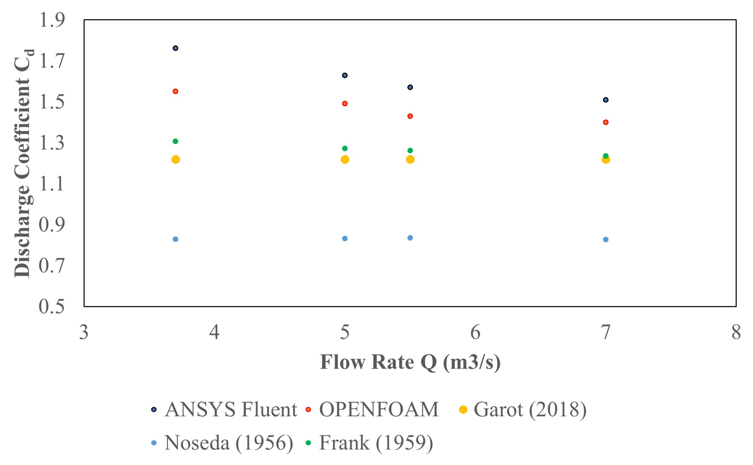
The efficiency of the intake structure depends on several factors, such as the shape of the bars, net spacing between them (void ratio), amount of flow and flow conditions, initial flow depth, and angle and length of the rack. Many researchers have conducted studies to design the minimum rack area required to transmit the maximum flow rate (Garot [1]; Bouvard [2]; Kuntzmann and Bouvard [3]; Noseda [4]; Noseda [5]; Noseda [6]; Mostkow [7]; Brunella et al. [8]). There are some assumptions in these studies; the flow on the rack is one-dimensional, the flow gradually decreases, the hydrostatic pressure distribution acts on the rack in the flow direction, and the energy level or energy head is constant along the rack. There are two approaches to the constant energy head; the energy level is either parallel to the river surface or to the slope of the rack. The orifice effect is one of the most important mechanisms for managing water withdrawal in the intakes, and the proportion of directed flow, $q_{intake}$, can be expressed by Equation (1):

$$q_{intake}=\frac{dq}{dx}=Cm\sqrt{2gH},$$

(1)

where $q_{intake}$ is the diverted discharge through the bottom rack per unit of length x, C is the discharge coefficient, m is the void ratio (the ratio of the opening area of the screen), and H is the hydraulic head. Many researchers’ experimental work has further developed equations for the discharge coefficient (Garot [1]; Noseda [6]; De Marchi [9]; Frank and Von Obering [10]; Dagan [11]; García [12]), which plays an important role in intake design. Researchers have shown that the value of the discharge coefficient depends on certain parameters; in particular, the shape, geometry, and spacing between bars are significant dimensions of the discharge coefficient (Righetti et al. [13]).

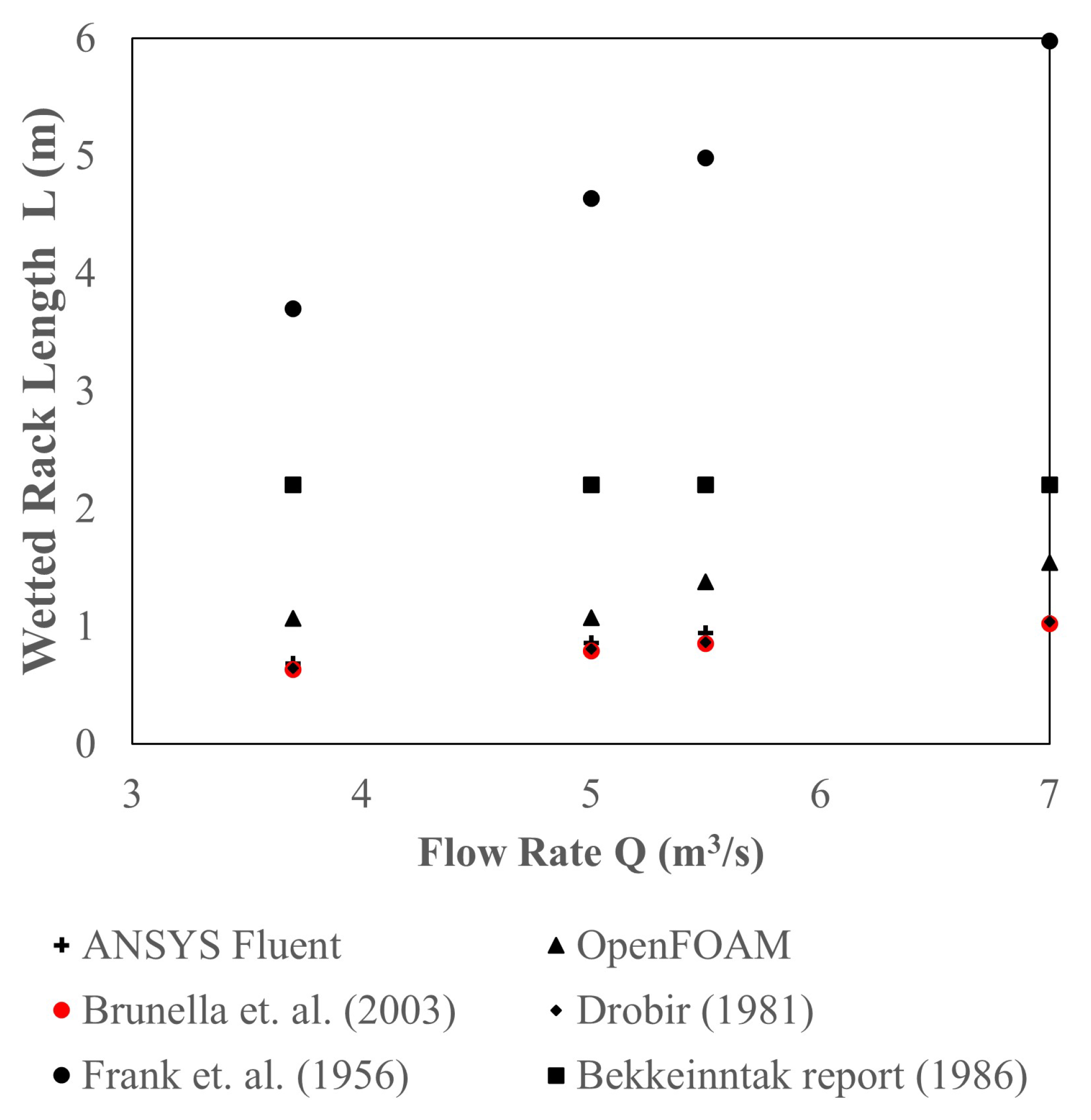
Another parameter that plays an important role in intake design is the minimum required wetted rack length. There are studies in the literature that consider the theoretical application of 1D energy and momentum conservation equations for wetted rack length calculation (Kuntzmann and Bouvard [3]; Noseda [5]; Frank and Von Obering [10]). More recently, based on the aforementioned studies, researchers performed laboratory experiments for wetted rack length and produced empirical correlations (Brunella et al. [8]; Castillo et al. [14]). In these studies, the researchers carried out experiments with differently shaped bars and defined the discharge coefficient.

Table 1. Intake unit discharge equations taken for the study from the literature.

Reference	Orifice Equation	Wetted Rack Length $\mathit{L}\left(\mathit{m}\right)$	Discharge Coefficient C
Garot [1]	$dq/dx=C_{d}m\sqrt{2gQ}$		$C_d=\sqrt{\frac{1}{{\left(\frac{b_1}{b_1+b_w)}\right)}^2\beta {\left(\frac{b_w}{b_1}\right)}^{\frac{4}{3}}}}$
Noseda [6]	$dq/dx=C_{d}m\sqrt{2gh}$	$L=\frac{1.848h}{C_{d}m}$	$Forsubcriticalflow:$  $C_d\left(h\right)=0.66{\mathrm{m}}^{-0.16}{\left(\frac{h}{l}\right)}^{-0.13}$
			$Forcriticalflow:$  $C_d\left(h\right)=0.78{\left(\frac{h}{l}\right)}^{-0.13}$
Frank et al. [10]		$L=\frac{2.561q}{C_d\sqrt{h}}$	$C_d\left(h\right)=1.22C_{qh}\left(h_0\right)$
Drobir [15]		$L=\frac{0.846h}{C_{d}m}$
Brunella et al. [8]	$dq/dx=C_{d0}m\sqrt{2ghcos\theta }$	$L=\frac{0.83h}{C_{d}m}$
Bekkeinntak Report [16]		$L=\frac{Q}{C_d{h}^{3/2}}$	$C_d=1.7\sim 2.1$

summarizes the equations in the literature and those used in this study.

Laboratory experiments or adequate computational fluid dynamics (CFD) simulations for intakes are rare because of the complex geometry and high cost of accurate numerical investigations. Studies in the literature consider a two-dimensional perspective on the vertical plane of the rack. However, in reality, the flow is three-dimensional, and in this case, CFD models, once validated against experimental values, can help to better understand the phenomenon (Bombardelli [17]; Blocken and Gualtieri [18]). While most researchers modelled the intake structure in one or two dimensions, only a few researchers examined the study in three dimensions (Bombardelli [17]; Castillo et al. [19]; Carrillo et al. [20]). However, there are very few studies in the literature modeling the water intakes. In addition, different simplifications were used in these studies. No reported study has modelled the brook intake together with the natural riverbed topography.

This study aimed to determine the behavior of the three-dimensional flow over the existing water intake structure under various flow rates using the CFD-VOF method. A further aim was to investigate measures to improve and optimize existing Tyrolean intake. Two different CFD finite volume codes were used for the simulations, ANSYS Fluent and OpenFOAM, and their performance was compared in terms of time and cost, as well as the effort spent. Previous studies numerically simulated with ANSYS CFX were conducted with circular bars or T-shaped bars (García [12]; Castillo et al. [19]; Carrillo et al. [20]). In our current contribution, we focused our attention on a rack consisting of rectangular bars. The physical behavior of the flow profile on the wetted rack was determined and the rack length values were compared with those in previous studies.

2. Project-Related Background

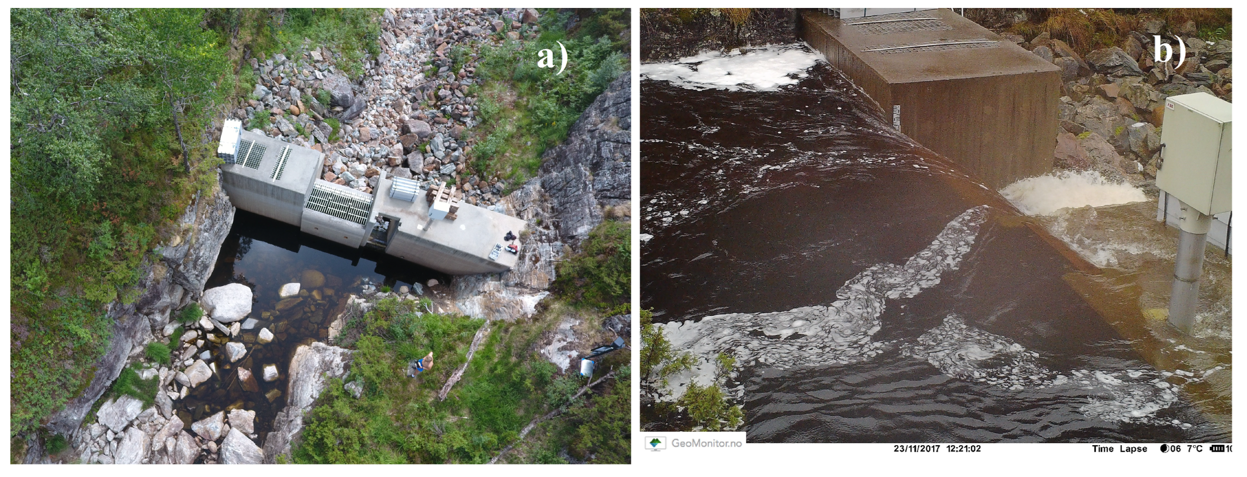
A case study has been selected, namely the Stigansåni brook intake, which is constructed as a Tyrolean weir, located in Southern Norway with coordinates Euref89 UTM33 6528477N 23422E. The elevation of the inflow weir is at 523.5 m.a.s.l. and the winter season generally lasts from December to March. This brook intake diverts water into the headrace tunnel of the 960 MW Tonstad HPP and is owned and operated by Sira-Kvina kraftselskap. Figure 1 includes a site map that shows the location of Tonstad HPP. This brook intake is found to have insufficient capacity and periods of water spilling every year. This intake type was selected as being among the most common intake designs in Norway. The Stigansåni brook intake diverts water from a 5 km² catchment with an annual inflow of 11 million m³ with mean discharge $Q_m=5$ m³/s. The water is directed into the headrace tunnel of the 960 MW Tonstad power plant, which is also diverted towards the Åna-Sira power plant further downstream. The annual production of the diverted water equals about 12 GWh. 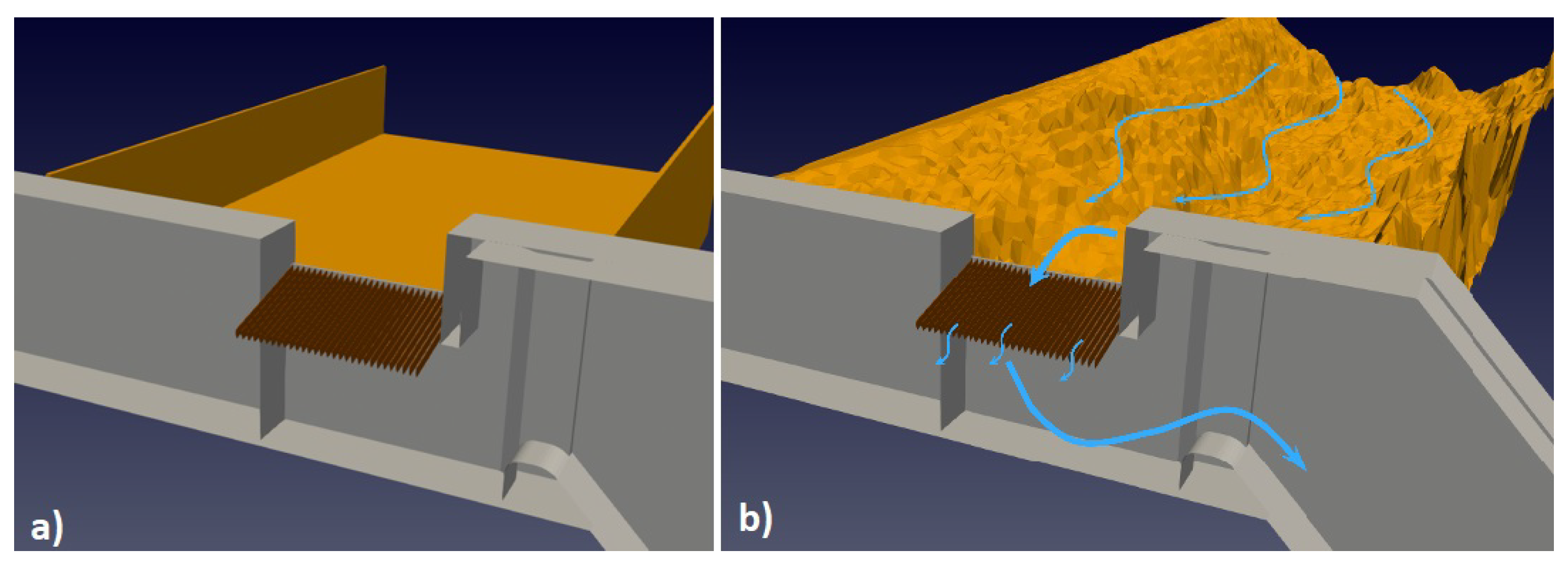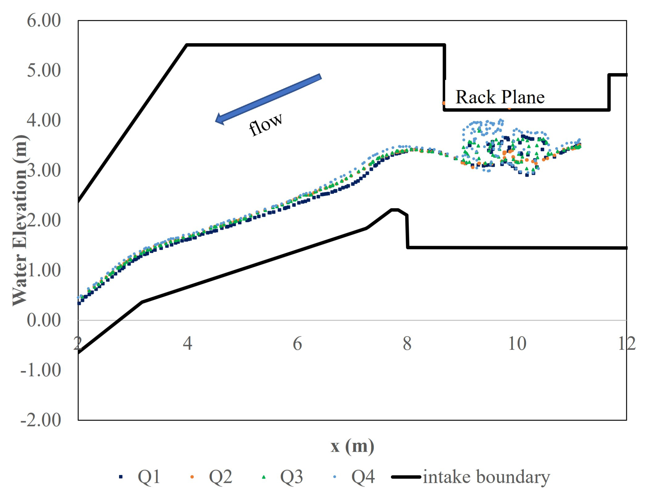As can be seen in Figure 1, this intake experiences both extremes of dry and wet conditions. The hydrograph of the catchment area is characterized by flash floods from extreme participation or sudden snow-melting events. Figure 1b shows a situation with water loss, where the intake is saturated, and water spills over both the intake rack and also over the concrete weir. This situation occurred during the winter, as heavy rainfall coincided with a temperature rise and the resulting snow melt. Such events are typical in this region and occur several times annually at this intake. The power plant owner is interested in investigating potential measures to increase the capacity of this intake.

3. Numerical Modeling

The subject of this research is the simulation of an intake with racks set in a natural riverbed topography under multiphase flow conditions, which represents a complex problem in fluid mechanics. A key challenge is modeling the relatively large river flows with larger mesh sizes, with the added intricacy of modeling the intake with racks, which feature relatively small and particularly narrow rack spacings within the riverbed. In order to obtain a highly accurate simulation, it is important to select the appropriate number of cells in the fine network created in the rack region of the water intake structure.

Simulations were performed using the finite-volume method (FVM) and commercially licensed CFD solver ANSYS Fluent with open-source platform OpenFOAM program used to compare the reliability and performance of the analyses. Both programs are widely used in research institutions. In this study, the current state of the existing Tyrolean intake was analyzed with the minimum amount of data from the study site necessary to perform 3D hydrodynamic modeling in several flow conditions. For this purpose, easy-to-access remote sensing photos were used as modeling input. First, a high-resolution Digital Elevation Model (DEM) from Google Earth satellite images was used to create the upstream and downstream river terrain of the Stigansåni intake area. For detailed topography of the inside of the riverbed, these images were supported with 3D scanning drone images. The DEM file extracted from the satellite images was transferred to the Autocad CIVIL 3D environment, and used to create a 3D triangular model of the riverbed as an .stl file. Secondly, the .stl file was further used in the ANSYS Space Claim software and also in OpenFoam. In ANSYS Space Claim, when created from remote sensing photos, this type of file is generally of good quality, but due to the nature of the topography, there may be frequent spikes or missing faces and holes in the terrain. The knit was checked with ANSYS Space Claim and the .stl file was repaired in the process of creating the geometry. The spikes in the field were softened by 40% shrink-wrap and the holes were closed. This approach also facilitates the meshing step, performed in the advanced stages. Thirdly, the existing structural project of the Stigansåni brook intake was redrawn in 3D in the CAD environment and the .stl file of the structure was saved as a separate file. Finally, the structure was added to the river topography prepared in the ANSYS Space Claim and the 3D full-scale geometry of the area to be modelled was created. A “fluid domain” was defined to represent the riverbed, and the intake body was added. The meshing process simply involved the combination of the two .stl files from the terrain file and from the intake structure in the OpenFoam environment.

In order to model river flows in 3D, the three-dimensional Reynolds-averaged Navier–Stokes equations involving conservation of mass and momentum need to be solved, assuming the flow is incompressible. Continuity and momentum equations for x, y, and z are given in Equations (2) and (3):

$$▽.u=0,$$

(2)

$$\rho \left(\frac{\partial u}{\partial t}+u.▽u\right)=-▽P+\mu {▽}^{2}u-\rho ▽.\left(\overline{u^{\prime }}{u}^{\prime }\right)+F,$$

(3)

where u is flow velocity, ▽ is divergence, $\rho$ is density of water, P is pressure, $\mu$ is dynamic viscosity, and F is gravity force.

In this study, the Eulerian multiphase approach was used to solve the air and water two-phase flow. Air was defined as the primary phase, and water as the secondary phase, representing the open channel flow. The material properties of both phases were introduced separately, and their densities were taken as $1.225$ kg/m³ and $998.2$ kg/m³, respectively. The surface tension modeling considers the surface tension force as a volume force concentrated at the interface. A surface tension coefficient of 0.072 N/m was specified. No wall adhesion was considered. In the ANSYS Fluent model, the viscous flow model was activated with the $k-\Omega$-based Shear-Stress Transport (SST) model (Menter [21]), which solved the Reynolds-averaged Navier–Stokes (RANS) equations. On the other hand, with OpenFOAM, the $k-\epsilon$ turbulence model was used and the interFoam solver was chosen to characterize the free surface flooding at the Stigansåni inlet. Both phases in the Eulerian flow model were considered as continuous fluids. The sum of the volume fractions $\left(r\alpha \right)$ of the air and water phases was 1 in each control volume. Cells with $0.5$ air volume fraction were considered as the free water surface. The time-dependent volume fraction formulation was used, and the volume fraction was obtained with an explicit formulation, such that the Courant number was $0.25$ in each time step. Second-order discretization schemes were used to solve the divergence and gradient.

Table 2. Comparison of ANSYS Fluent and OpenFOAM simulation times and model implementations.

	ANSYS Fluent	OpenFOAM
Domain Size:	10 m × 10 m	10 m ×15 m
Elements:	$2.8\times {10}^6$	1∼3 × ${10}^6$
Turbulence Model:	RANS $k-\Omega$ (SST) model	RANS $k-\epsilon$ model
Wall function:	Standard wall function [22]	Standard wall function [22]
Solution Methods
Gradient:	Second-order least squares	Second-order least squares
Divergence:	Second-order upwind	Second-order upwind
Turbulence Kinetic energy:	Second-order upwind	Second-order upwind
Time derivative:	First-order implicit	First-order implicit
Multiphase model:	VoF	VoF
Interface capturing method:	SIMPLEC	SIMPLEC
Pressure–velocity coupling:	PISO	PISO
Simulation Time:	300 s	100 + 20 s
Parallel Computing:	32 Core	32∼48 Core
Computation Time:	72 h	24 h

shows a comparison of model applications and simulation times used for the two solvers.

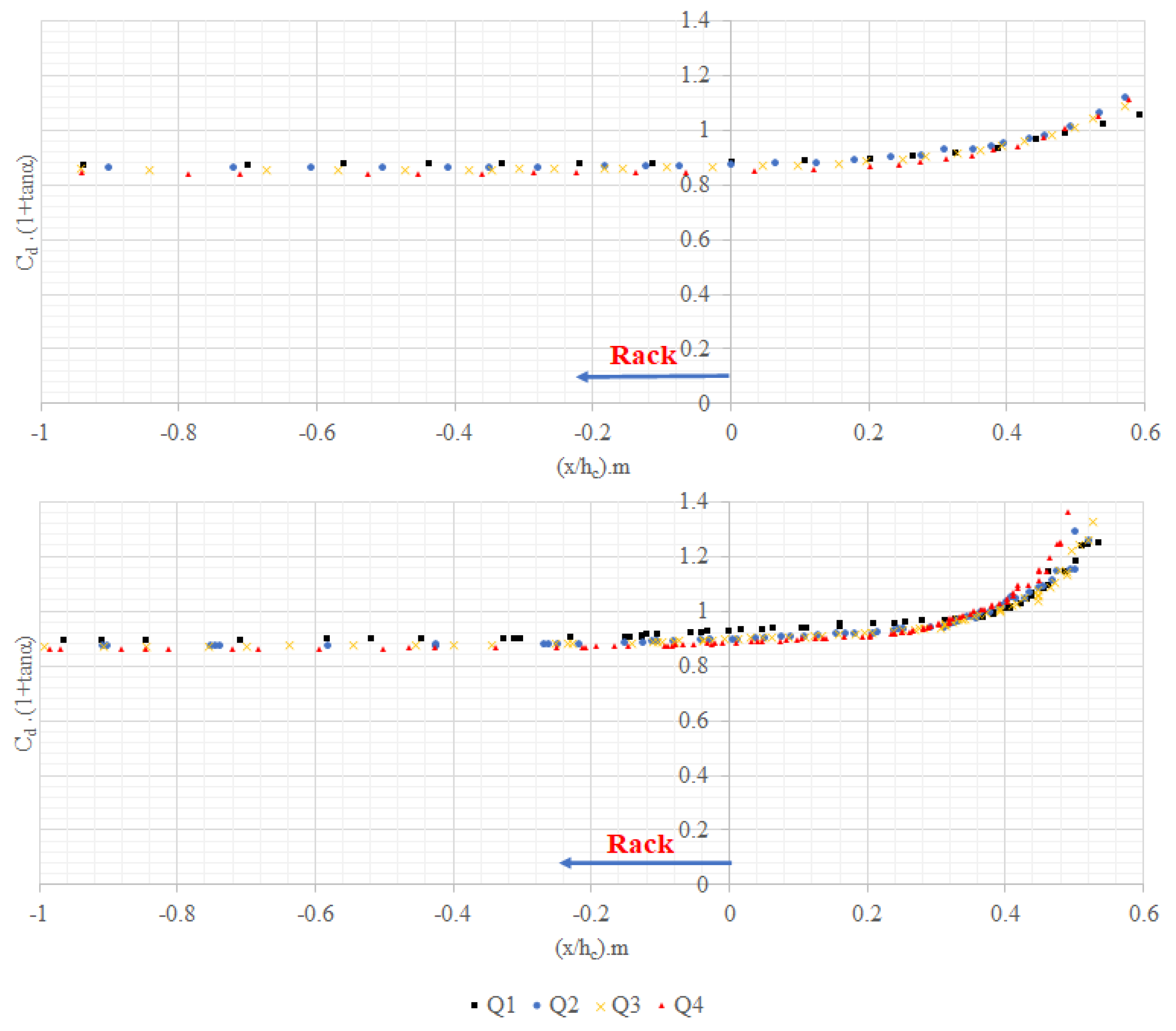
Simulations were performed with four specific flow rates for Stigansåni intake that were selected based on reports from NVE (the Norwegian Water Resources and Energy Directorate). All flow rates were operated under steady flow conditions of 300 s for ANSYS Fluent and 100 + 120 s for OpenFOAM simulations (for initial flow development with low-resolution domain and for high-resolution simulations, respectively). The river velocity inlet boundary condition values for each flow rate are given in

Table 3. Inlet boundary conditions.

Test No	Q (m3/s)	v (m/s)
Q1	$3.7$	$0.18$
Q2	5	$0.25$
Q3	$5.5$	$0.27$
Q4	7	$0.35$

Q is the flow rate; v is the river inlet velocity.

below.

3.1. Domain Model with ANSYS Fluent

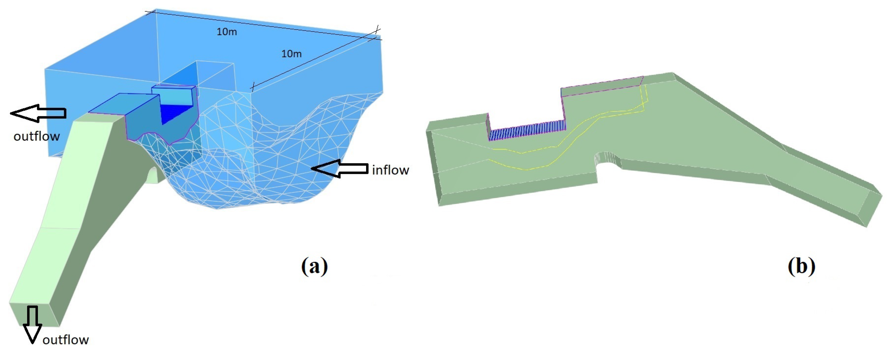
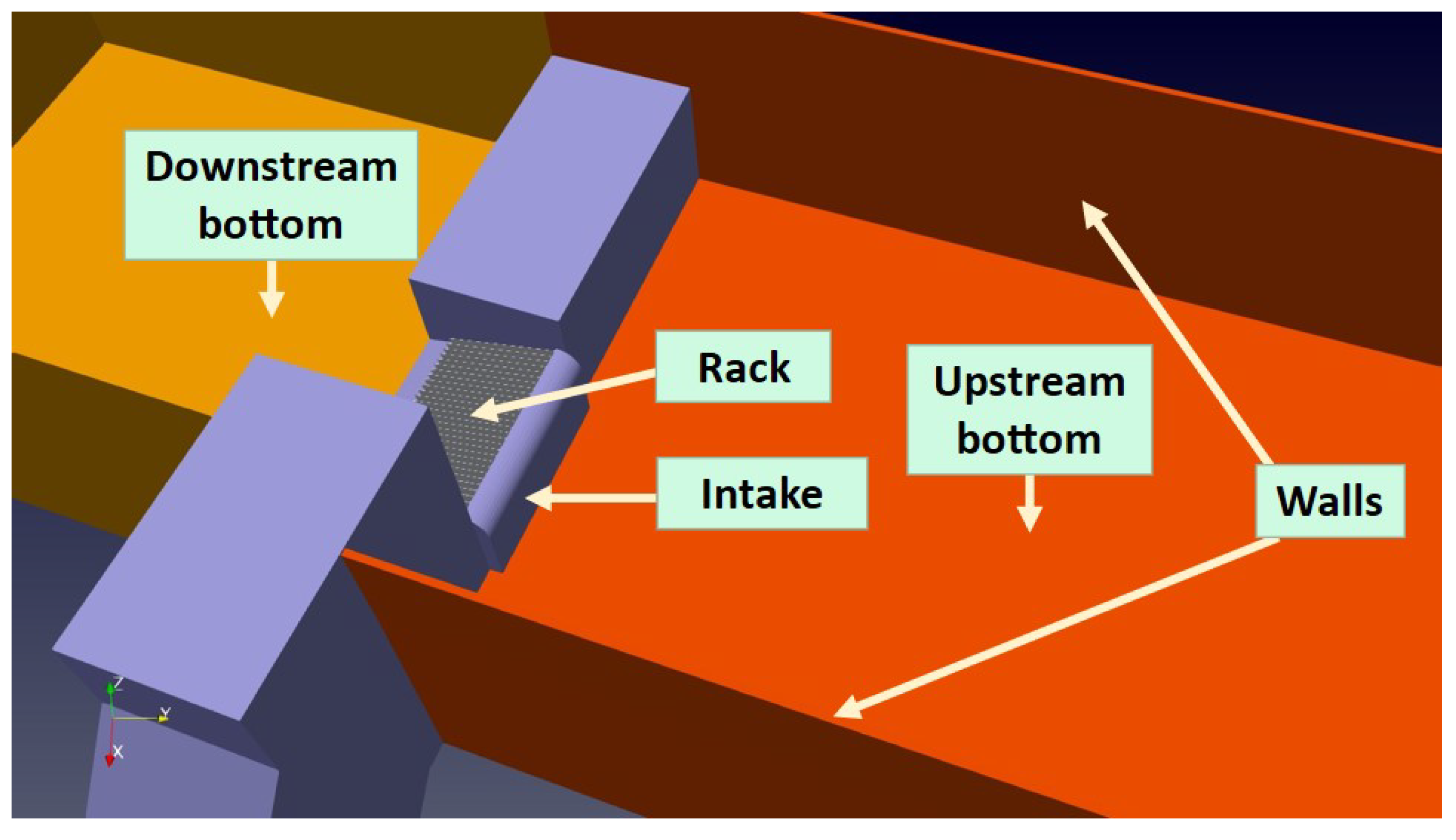
After connecting the water intake structure in the CAD and the river topography prepared in the ANSYS Space Claim, a 10 m × 10 m “fluid area” was defined to represent the riverbed. These consist of two parts, the flow area and the water intake structure, as seen in Figure 2.

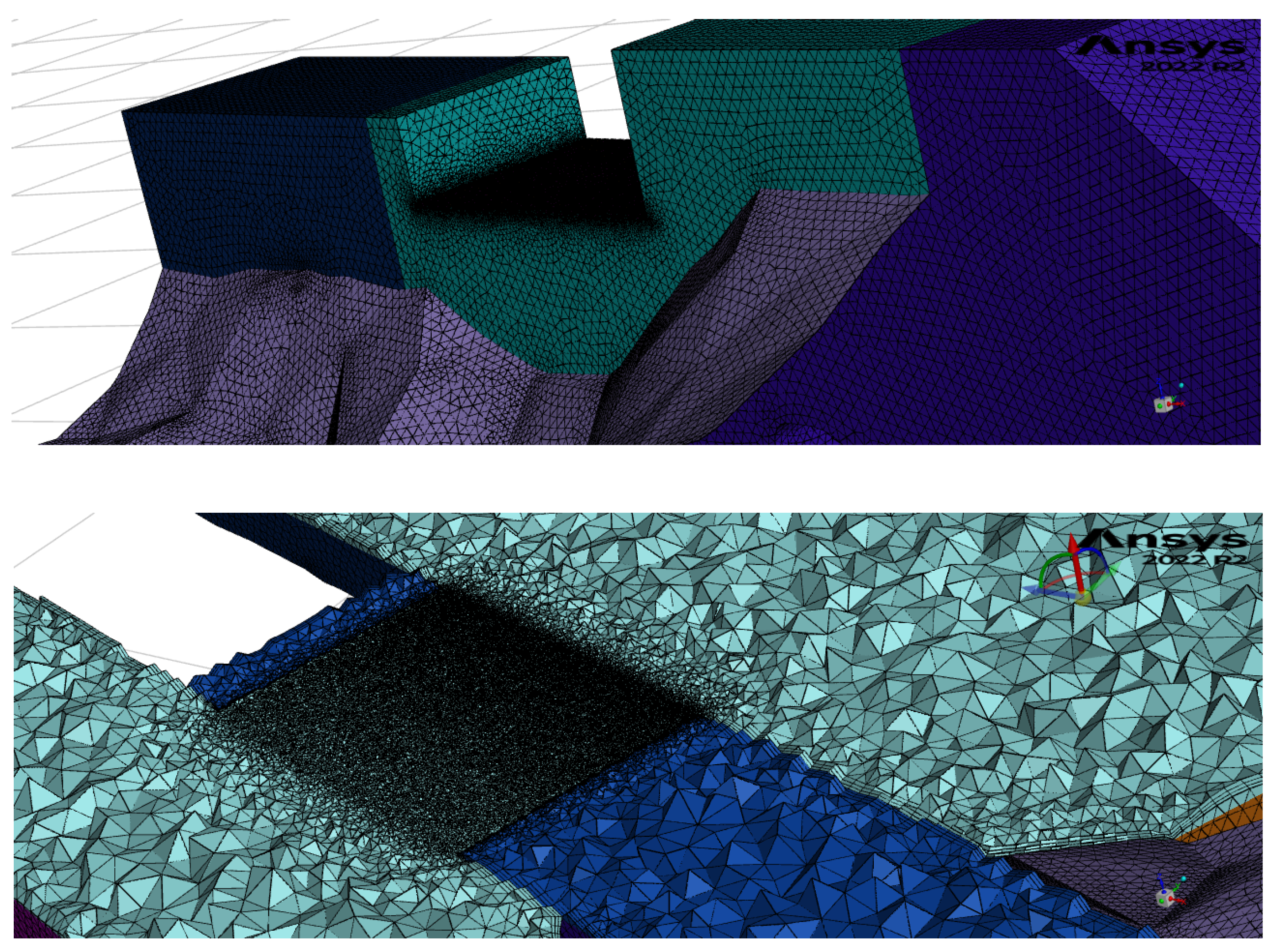
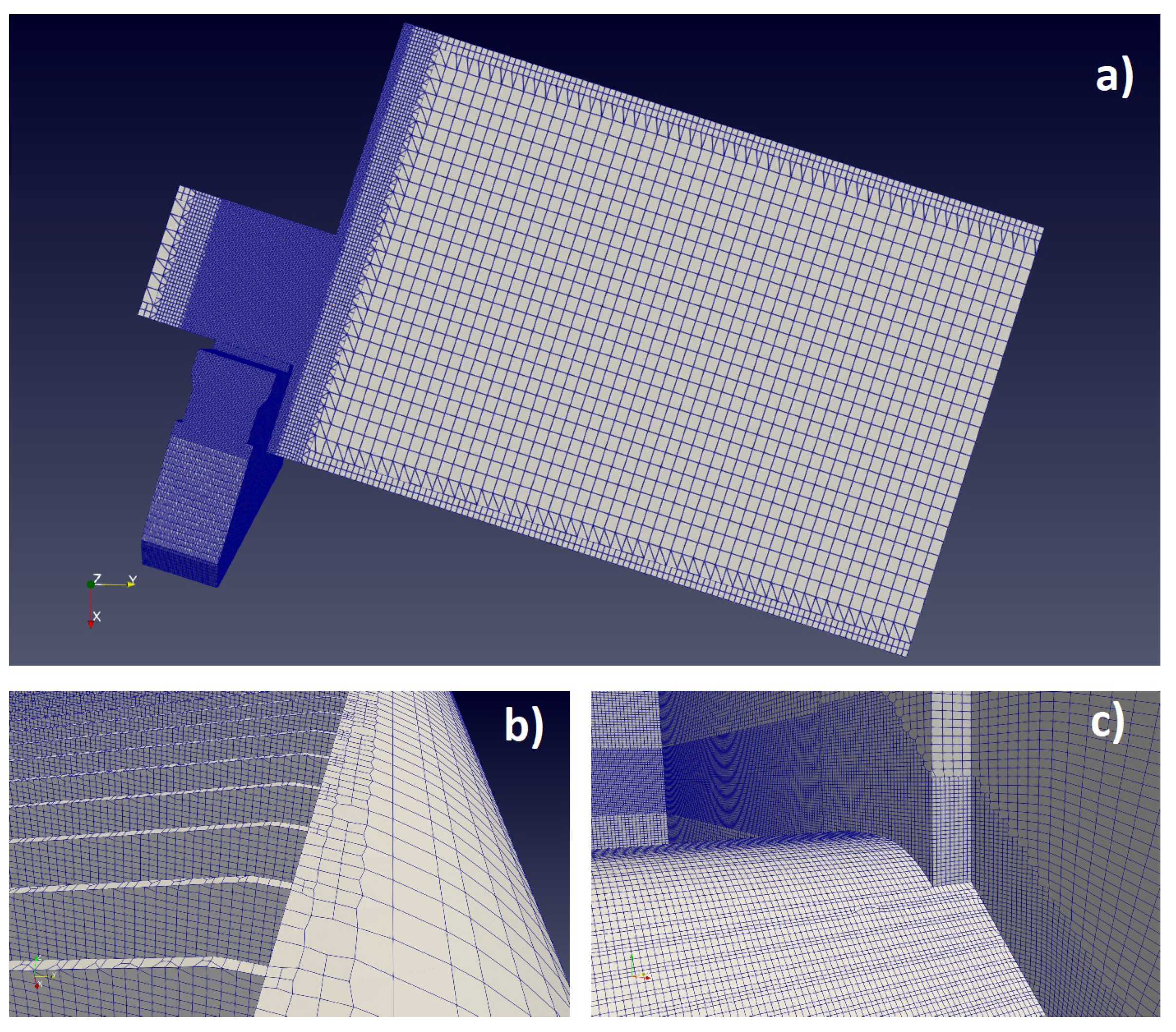
The meshing of the domain was performed via the ‘sweep’ method for the bottom rack to the brook intake, and the brook intake to riverbed, and the “tetrahedral” meshes for the fluid domain to obtain mesh cells due to the complex geometry (ANSYS [23]). The generated mesh of the fluid domain consisted of approximately $2.8\times {10}^6$ cells, $13\times {10}^6$ faces, and $8.1\times {10}^6$ nodes, which means each cell size is sufficiently small relative to the approximate rack grids assigned in simulations. In the simulations, the minimum curvature mesh element size was taken as 1 $\mathrm{mm}$, which is smaller than the rack grid in the intake, and this cell size was applied to the denser mesh at the level of the bottom rack. The denser mesh was applied with smaller cell sizes in areas where the intake was. The bottom rack and intake into the riverbed were densely dispersed through the domain, and the cell sizes were increased towards the edges, to avoid unnecessary mesh density. Regarding the mesh quality of the prepared geometry, the maximum aspect ratio, average skewness, and averaged orthogonal quality criteria were calculated as 24, $0.025$, and $0.71$, respectively. According to the obtained values, the model is considered to have good mesh quality (Figure 3).

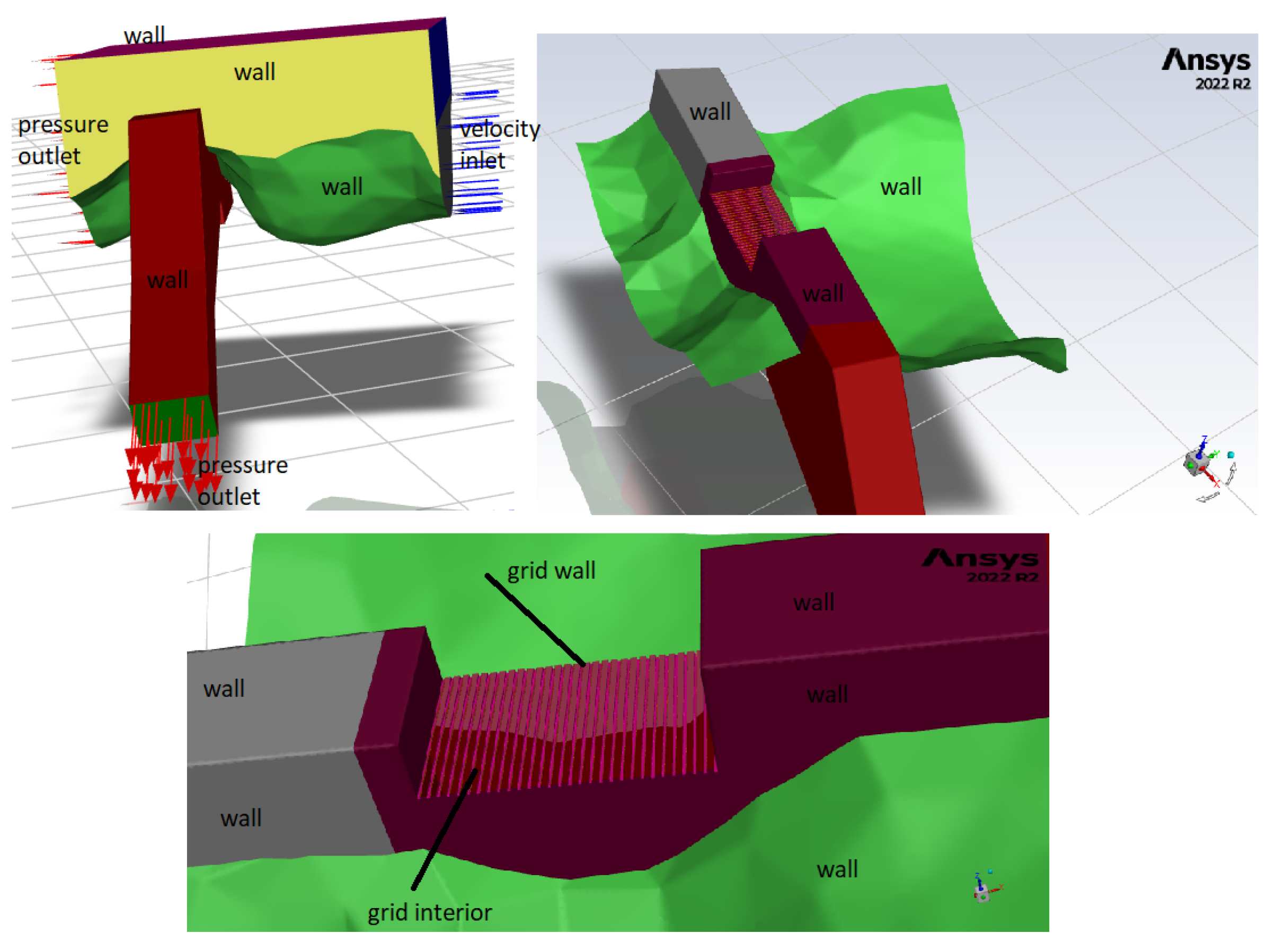
As for the boundary conditions, the upper river-free surface of the meshed fluid area was simplified as the no-slip wall conditions. The outlet of the river fluid domain and the outlet of the intake structure were defined as the “pressure outlet” boundary condition, with a relative pressure of 0 Pa. This is based on previous flow observations, as the river inlet boundary condition (NVE) modeling was conducted with four different flow rates at the entrance to the velocity inlet. In addition, the water volume fraction was taken as 1 and the air volume fraction as 0 in the inlet conditions, and this was simulated. The grid spaces of the intake structure were defined by the “interior” boundary condition between the river fluid domain and the intake fluid domain. Grids, as well as all other outer surfaces (riverbed, riverside surfaces, bottom, up and side surfaces of intake structure), were defined as the no-slip wall conditions (Figure 4).

The simulations were performed in double precision, and as transient flow using the Eulerian multiphase flow model. The solution method of pressure velocity coupling was chosen, combined with the SIMPLEC Scheme. Spatial discretization methods for solving the equation were applied as a second-order upwind scheme to increase the accuracy of the solution. Another crucial parameter influencing the accuracy and stability of numerical solutions is the length of the time step ($dt$), calculated using the LAX Finite Difference Scheme. The initial water level in the riverbed was defined within the domain’s fluid regions using the “patch” method in Fluent. Thus, at the start of the simulation, the water was positioned at the beginning of the water intake structure. Consequently, electing the time step for different Courant numbers involved a grid spacing of ($dx=0.001$ m), representing the minimum mesh size at the water intake structure. Test simulations were conducted with reasonable time steps and a Courant number in the range ($C\in [0.2,1.0]$) and a maximum speed of (0.35 m/s), with time steps ($dt\in [0.001,0.01]$). As a result of these tests, the time interval with Courant number is 0.25, which requires approximately 10 iterations for convergence at each time step, and this was selected as ($dt=1.25\times {10}^{-3}$ s). This selection aligns with values reported in the literature for numerical modeling of full-scale hydraulic structures (Torres et al. [24]). Given the small time step and the large number of meshes, it was necessary to use a workstation capable of parallel computing for Computational Fluid Dynamics (CFD) simulations. The model was simulated over a total of 300 s, and it took approximately 72 h to model one scenario, running on 32 cores on an Nvidia RTX A5000 workstation with 1024 GB of memory.

3.2. Domain Model with OpenFOAM

The simulation domain was defined differently as for modeling with ANSYS Fluent. The upstream end of the OpenFOAM domain was set approximately 15 m upstream of the intake structure, but only a few meters downstream (in both directions: from the intake tunnel towards to the HPP, and from the downstream part of the watercourse) (Figure 5).

A high-resolution topological survey was available at the area around Stigansåni. At the original bathymetry, various polyhedra cell shapes would be generated during the meshing process that increase the size of the final computational grid (in terms of cell numbers), and the computation effort (in terms of resources needed to finish a simulation) necessary to achieve the converged hydraulic state. However, instead, a simplified topology was used. The flow condition over the intake rack structure is estimated to be free-flowing towards the downstream direction without any impact propagated towards upstream (i.e., backed hydraulic jump is not expected to form immediately above or downstream of the intake structure, neither is any blockage found at the downstream vicinity of the intake). At the upstream side, there is a need to test how the natural topology defines the approaching flow towards the intake compared to simplified surroundings. Thus, a comparison analysis was performed between two cases under the same conditions, but with different topology used upstream. The isometric views of the two topologies are presented in Figure 6.

The computational grid was generated with the snappyHexMesh utility of OpenFOAM. It generates hexahedra-dominant mesh on a user-defined domain. Finer mesh resolution was applied at the intake opening and near the inside weir (Figure 7). Depending on the different setups, the mesh size varied between $1\times 106$ and $3\times 106$ elements.

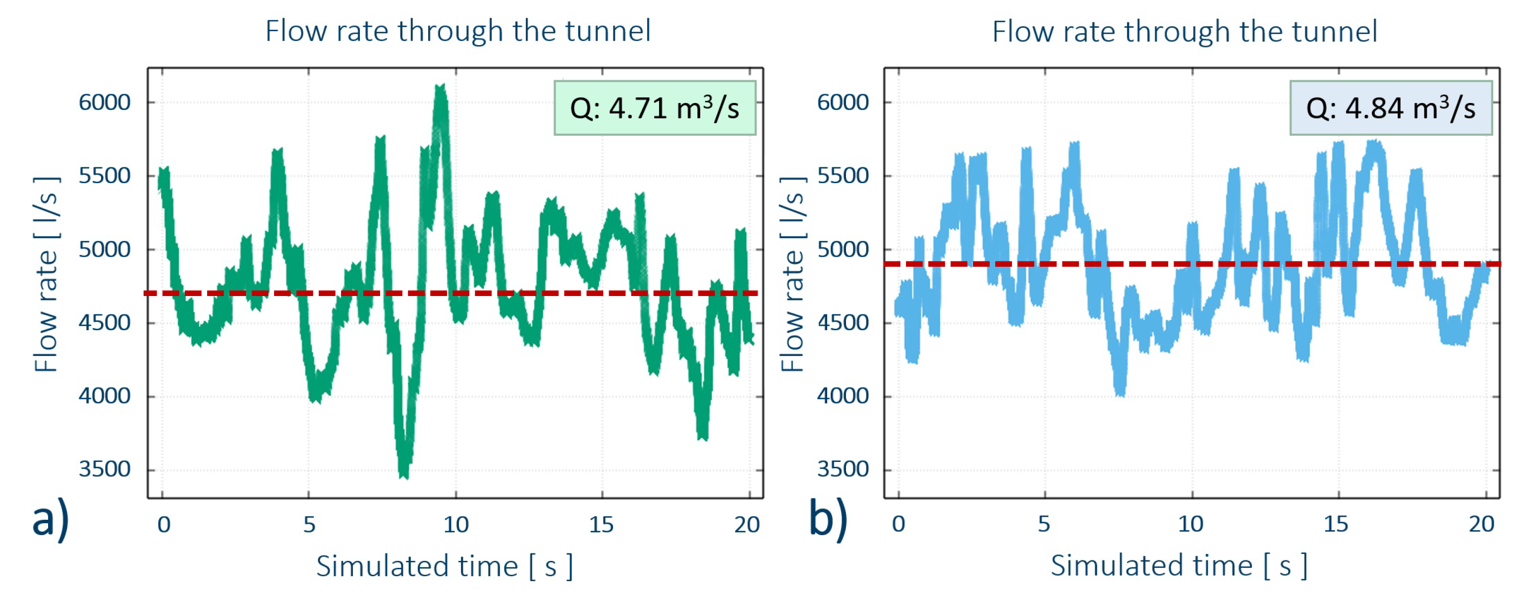
The modeling strategy with OpenFOAM was set on two levels. On the first one, the domain was meshed with moderate resolution. In addition, there was no rack structure defined at the intake opening in this case. Such simplifications spared significant computational effort in initializing the hydraulic conditions at the simulated domain. With a “cold-start” the simulation was set to fill up the upstream reach of the domain with a predefined flowrate (e.g., $Q=4.0$ m³/s) and let it overflow the intake opening. Flowrates were constantly monitored at three patches: inlet, outlet towards the HPP, outlet towards downstream. The first level of simulation was continued until flowrates through the outlets become constant over time. Simulated time varied between 80 and 100 s at the first level for the different simulated flowrates. Once hydraulic conditions were developed, it was used as an initial condition on the second level of modeling.

On this level, the domain that included the intake rack bars was meshed with a finer resolution. The simulation was run further on the finer setup following the same strategy with monitoring the flowrates through the outlets. The solution was monitored, showing that the intake overflow fluctuates over time. Upon reaching a hydraulic developed state, the simulation was run long enough to determine the statistical average of flowrates through the outlets. That time was set to 20 s and with that it takes 100∼120 s in total for simulation of a single case on the two levels. The length of the time step, ($dt$), calculated using the LAX Finite Difference Scheme, was selected as $dt=2.0\times {10}^{-3}$ s.

4. Results and Discussion

In Figure 8 and Figure 9, the longitudinal free surface depths inside the intake and results can be observed for four specific flows (Q1, Q2, Q3, and Q4), depending on the water volume fraction at 300 s for ANSYS Fluent and 100∼200 s for OpenFOAM simulations. The $0.5$ level of the water volume fraction shows the water levels.

The results obtained from OpenFOAM reveal that the water levels both inside of the intake and over the rack are approximately 15% to 20% higher for each inlet boundary condition. In Figure 9, the water levels inside the brook intake for four different flow rates are compared, and it is seen that the values are in harmony.

4.1. Wetted Rack Length and Flow Profile over the Rack

Figure 10 provides a comparison of the water levels over the rack for four different flow rates. It is seen that OpenFOAM simulations gave approximately 15% to 20% higher results.

To compare the flow profiles, the water depths were dimensioned using the critical depth $h_c$, the void ratio m, and the discharge coefficient $C_d$ (Brunella et al. [8]). Figure 11 shows the dimensionless flow profiles over the rack.

Considering the dimensionless profiles, if divided into two regions (i.e., pre-rack and post-rack) as $x/h_{c}m{C}_d>-0.75$ and $x/h_{c}m{C}_d<-0.75$, in general, similar behavior is seen for all flow rates. Although the two regions tend to show differences, their behavior can be explained by the following polynomial curve for $R^2>0.97$, which is similar to that described by Carrillo et al. [20]:

$$\frac{h}{h_c}=a{\left(\frac{x}{x_c}m{C}_d\right)}^4+b{\left(\frac{x}{x_c}m{C}_d\right)}^3+c{\left(\frac{x}{x_c}m{C}_d\right)}^2+d\left(\frac{x}{x_c}m{C}_d\right)+e,$$

(4)

Unlike [20], model results with OpenFOAM showed a logarithmic behavior over bar spacing:

$$\frac{h}{h_c}=aln\left(\frac{x}{x_c}m{C}_d\right)+e,$$

(5)

Since the pre-rack behaviors of ANSYS Fluent and OpenFOAM results were similar, coefficients with $R^2>0.91$ curve fit were calculated by averaging values. On the other hand, although their behavior over bar and over bar spacing shows the same mathematical expression, the coefficients are calculated separately because $R^2$ decreases. Curve fits are $R^2>0.99$ in this state. The coefficients of the fourth-degree polynomial expression obtained for the regions as $x/h_{c}m{C}_d>-0.75$ and $x/h_{c}m{C}_d<-0.75$ and over bar spacing are presented in

Table 4. Coefficients of the mathematical expressions for Equation (4).

$\mathbf{(}\mathit{x}\mathbf{/}{\mathit{h}}_{\mathit{c}}\mathbf{)}{\mathit{mC}}_{\mathit{d}}$		a	b	c	d	e
>−0.75		0.153	0.97	2.06	1.91	0.70
<−0.75 Over Bar		−0.071	0.30	0.42	0.24	0.61
ANSYS Fluent	<−0.75 Over Bar spacing	−0.02				0.11
OpenFOAM	<−0.75 Over Bar spacing	0.17				0.31

.

In order to create a design which optimizes the diversion of water from the river, the minimum wetted rack length should be accurately estimated (García et al. [25]). The minimum wetted rack length was defined by Drobir [15] as the distance from the beginning of the rack to the section where the nappe enters directly through the racks (measured between the bars). Figure 12 shows how the discharge coefficient $C_d$ is estimated for the brook intakes in Norway, according to the Bakkeinntak Report [16].

Table 5. Computed wetted rack lengths with various formulas from the literature.

Q (m3/s)	${\mathit{L}}_{1-\mathit{ANSYS}}$ (m)	${\mathit{L}}_{1-\mathit{OpenFOAM}}$ (m)	${\mathit{L}}_{1-}$[10] (m)	${\mathit{L}}_{1-}$[8] (m)	${\mathit{L}}_{1-}$[15] (m)	${\mathit{L}}_{1-}$[16] (m)
$3.7$	0.68	1.07	3.70	0.63	0.64	2.21
5	0.86	1.07	4.64	0.80	0.81	2.21
$5.5$	0.95	1.38	4.99	0.86	0.87	2.21
7	1.03	1.54	5.98	1.03	1.04	2.21

also shows how the minimum wetted rack length is calculated according to the Bakkeinntak Report [16]. When the discharge coefficient $C_d$ is chosen as $2.0$ on the safe side, the minimum wetted rack length is calculated as $2.2$ m, though it is 2.0 m in the current project. Table 5 shows the comparison of the $L_1$ values obtained from the numerical simulations and the values calculated from the three different equations available in the literature. It can be seen that Frank et al.’s [10] equation gives overestimated results compared to those from other methods. Very similar results were obtained from the methods of ANSYS Fluent, Brunella et al. [8], and Drobir [15]. It can be seen that the relationship between flow rate and wetted rack length exhibits a logarithmic behavior (Figure 13).

4.2. Discharge Coefficient and Water Capture Capacity

Although, theoretically, the discharge coefficient varies along the rack, formulas presented in the literature generally give average values for each rack.

Table 6. Computed discharge coefficients with various formulas from the literature.

Q (m3/s)	${\mathit{C}}_{\mathit{d}-\mathit{ANSYS}}$	${\mathit{C}}_{\mathit{d}-\mathit{OpenFOAM}}$	${\mathit{C}}_{\mathit{d}-}$[1]	${\mathit{C}}_{\mathit{d}-}$[6]	${\mathit{C}}_{\mathit{d}-}$[26]
$3.7$	1.76	1.55	1.22	0.83	1.311
5	1.63	1.49	1.22	0.83	1.271
$5.5$	1.57	1.43	1.22	0.84	1.26
7	1.51	1.40	1.22	0.84	1.24

shows the discharge coefficient values obtained by Frank and Von Obering [10], Noseda [6], and Garot [1]. Garot’s [1] formula is not flow parameter-dependent, and therefore, not affected by flow rate changes, but for the wetted rack length in the Noseda [6] formula, ANSYS Fluent values were used (all formulas in Ref. Table 1).

In Figure 14, discharge coefficient values and those obtained by Frank [26], Noseda [6], and Garot [1] equations and numerical results for different specific flows are compared.

Figure 15 shows the dimensionless variation in discharge coefficient across the rack under various flow rates for Stigansåni intake. The values obtained from both ANSYS Fluent and OpenFOAM were used for the current flow depths. The discharge coefficient changes before and after the rack, and along the rack. In Figure 15, the zero point is the start of the rack, and the change after this point is shown for rectangular profiles for Stigansåni intake. In the literature, remarkable differences were observed between the behaviors of T-shaped and circular bars (Castillo et al. [19] and Carrillo et al. [20]). The rack with circular bars has higher discharge coefficients than that with T-shaped bars. The results of the current research show that rectangular-shaped bars have higher discharge coefficients than both circular and T-shaped bars. It should be noted that the studies were carried out in clear water conditions without sediments.

The behavior of the non-dimensional discharge coefficient in Figure 15 can be mathematically expressed by the following Equation (6) for rectangular bars. The a and b coefficients found for this study are presented in

Table 7. Coefficients of the mathematical expressions for Equation (6).

${\mathit{C}}_{\mathit{d}}$	a	b
$C_d=\frac{a{e}^{b\left(\frac{x}{h_c}m\right)}}{1+tan\alpha }$	1	0.0463

.

$$C_d=\frac{a{e}^{b\left(\frac{x}{h_c}m\right)}}{1+tan\alpha },$$

(6)

In the analyses with OpenFOAM, it was observed that the water levels on the rack upstream and on the rack were higher than the results obtained from ANSYS Fluent. Therefore, more water passed downstream of the structure and the amount of water entering the intake decreased by approximately 10%, especially when the flow rate increased ($Q=7$ m³/s). Flow rates taken into intake calculated with numerical models are given in

Table 8. Flow rates calculated with numerical models.

Q (m3/s)	${\mathit{Q}}_{\mathit{ANSYSFluent}}$ (m3/s)	${\mathit{Q}}_{\mathit{ANSYSFluent}}$ (%)	${\mathit{Q}}_{\mathit{OpenFOAM}}$ (m3/s)	${\mathit{Q}}_{\mathit{OpenFOAM}}$ (%)
$3.7$	3.23	87	3.61	98
5	4.48	90	4.36	87
$5.5$	4.68	85	4.84	88
7	6.08	87	5.23	75

.

The marginal difference was spotted in simulations with simplified and with natural topology tested with OpenFOAM. With $Q=5.5$ m³/s inlet flow, the modelled flowrate averaged over time at the outlet patch towards the HPP shows a 3% difference between the two cases in Figure 16. The case with simplified surrounding slightly underestimates the flow rate at the intake outlet, that has been accepted for performing further model simulations on the simplified domain.

The water capture capacity factor of the Tyrolean weir is calculated according to Yilmaz [27] and Yildiz et al. [28]:

$$WCC=Q_{wi}/Q_{wT},$$

(7)

where $Q_{wi}$ is the diverted discharge flow through the racks, and $Q_{wT}$ is the total discharge of the approaching main river flow. Figure 17 presents the water capture capacity curve of Stigansåni intake for ANSYS Fluent and OpenFOAM numerical model results under different flow rates. In the simulation with OpenFOAM, the higher water capture capacity factor was calculated at lower discharges. An increase of approximately 50% from the average value of $Q=5$ m³/s increases the water passing downstream of the intake, and the amount of water entering the structure decreased by 10% compared to the ANSYS Fluent results. It is seen that while the discharge $Q_{wT}$ increases, the water capture capacity factor gradually decreases ($Q_{wi}/Q_{wT}$). On the other hand, this may be due to the greater number of meshes in the ANSYS Fluent model compared to OpenFOAM.

5. Conclusions

This study aimed to fill the literature gap in numerical estimation of the hydraulic flow over existing Tyrolean intake using the existing natural riverbed topography. In addition, the study has included a comparison of results from ANSYS Fluent (commercial) and OpenFOAM (freeware), which were both used in the project. The simulation results showed the following:

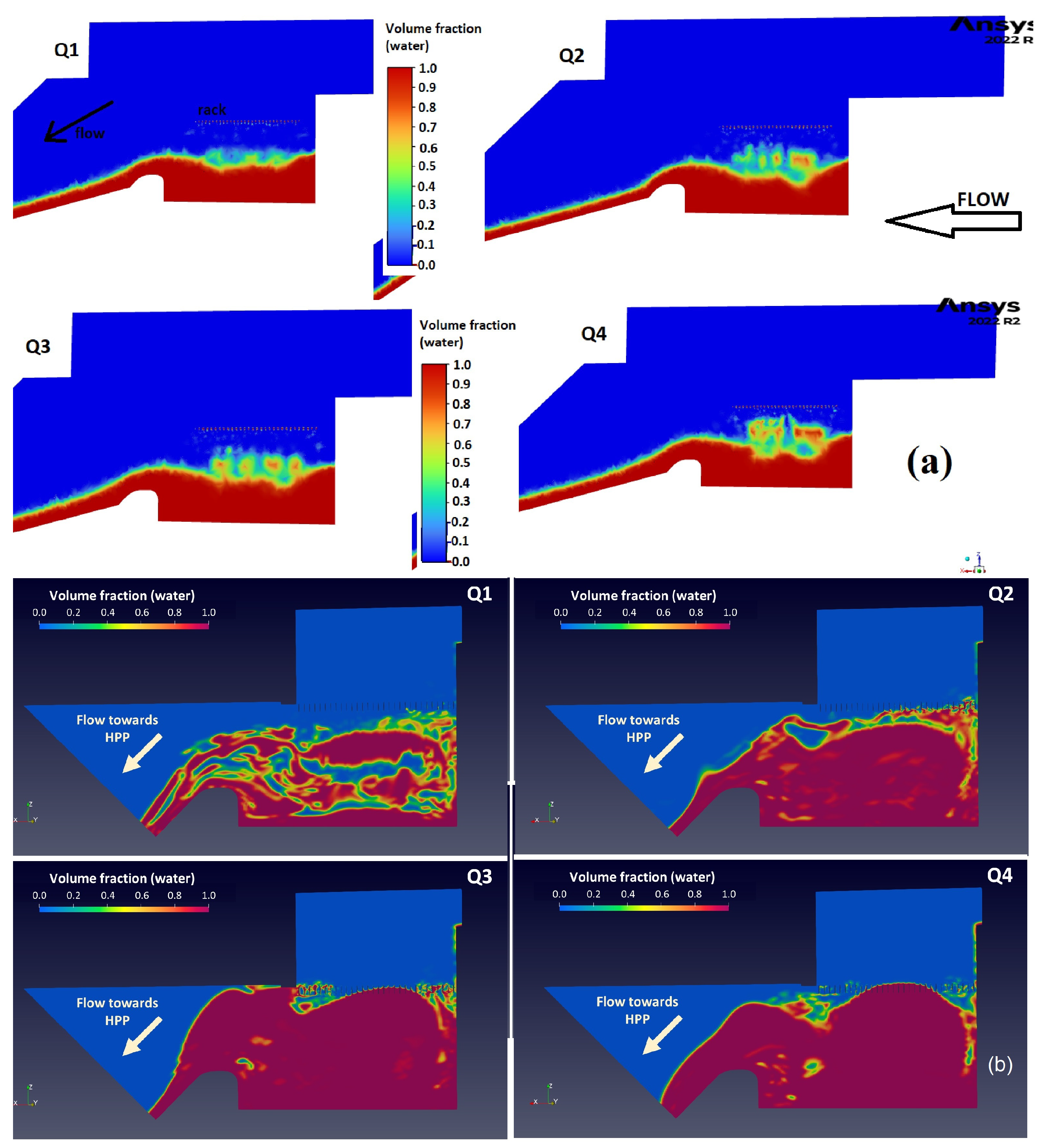
• CFD methods offer fast, practical, and inexpensive solutions for investigating the efficiency of existing systems. Modeling can be cost-effective with limited input data, and still have sufficient accuracy.
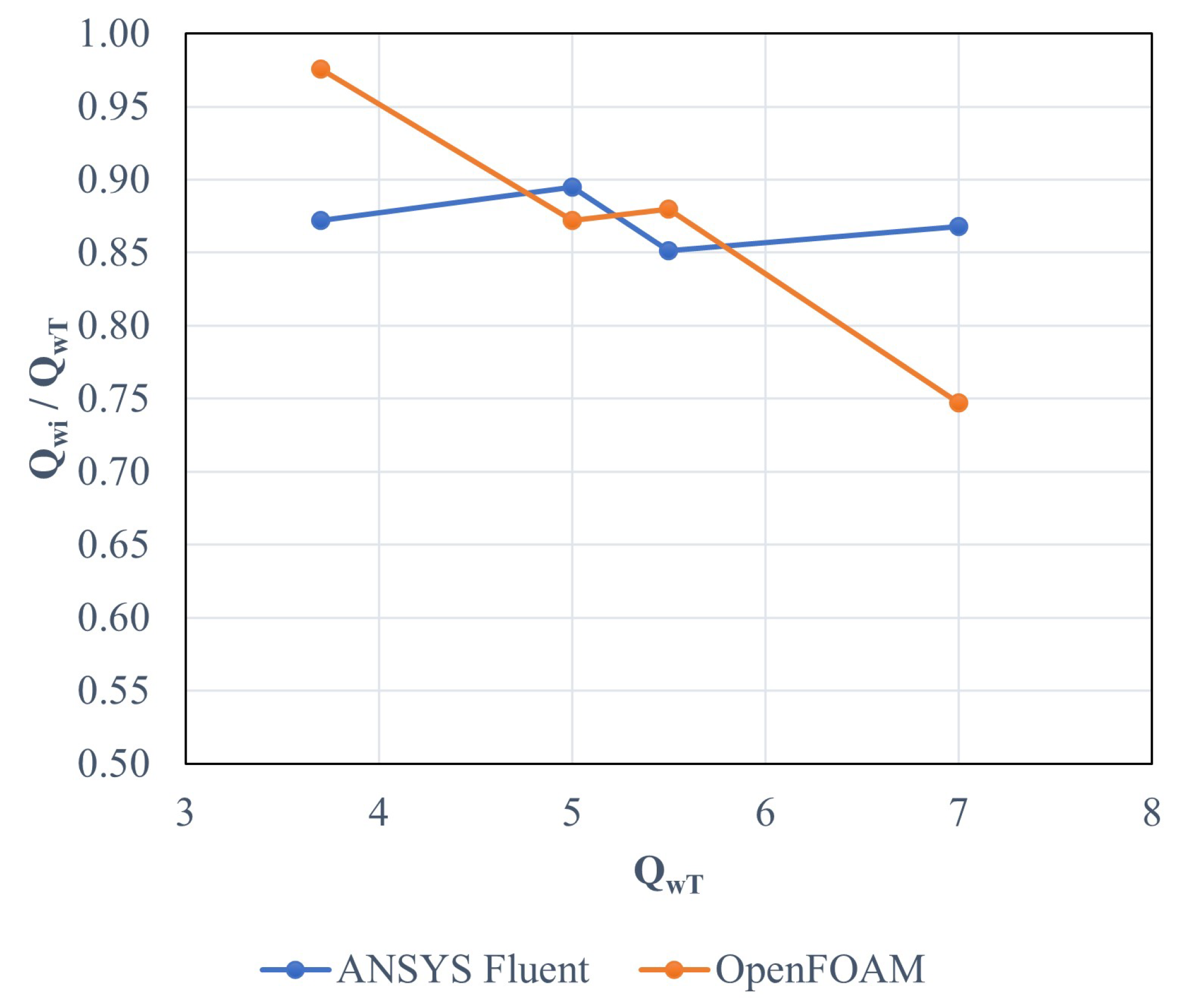
• Simulations for four different flow rates yielded 15–20% higher water levels in the VOF model applied in OpenFOAM compared to the simulations in the VOF model applied in ANSYS Fluent. Consequently, while higher water capture capacity was calculated at lower discharges according to the OpenFOAM simulations, 10% less water capture capacity was found at higher discharges compared to ANSYS Fluent results. On the other hand, the current behaviors of the VOF model applied in ANSYS Fluent were found to be compatible with the literature.
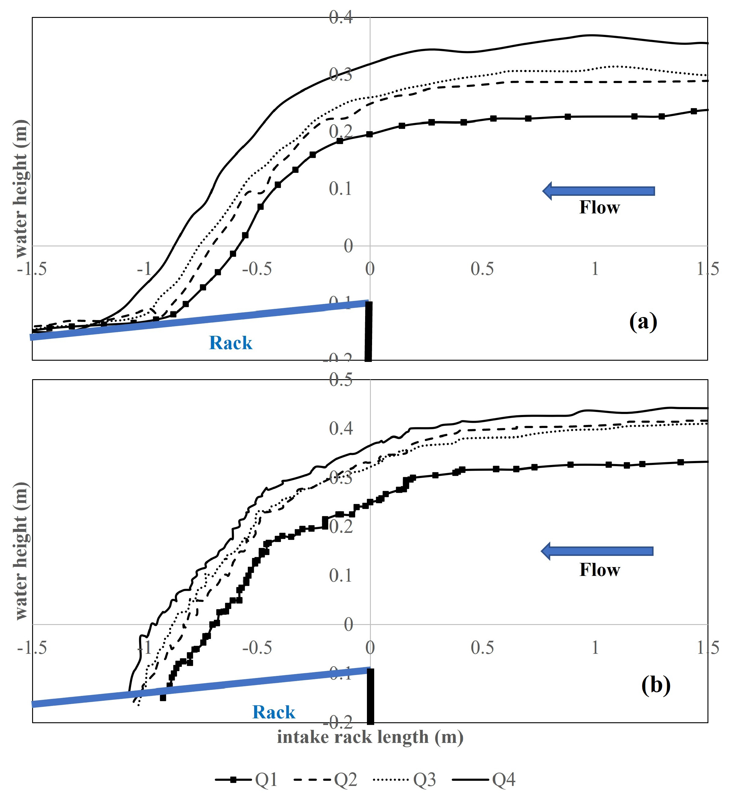
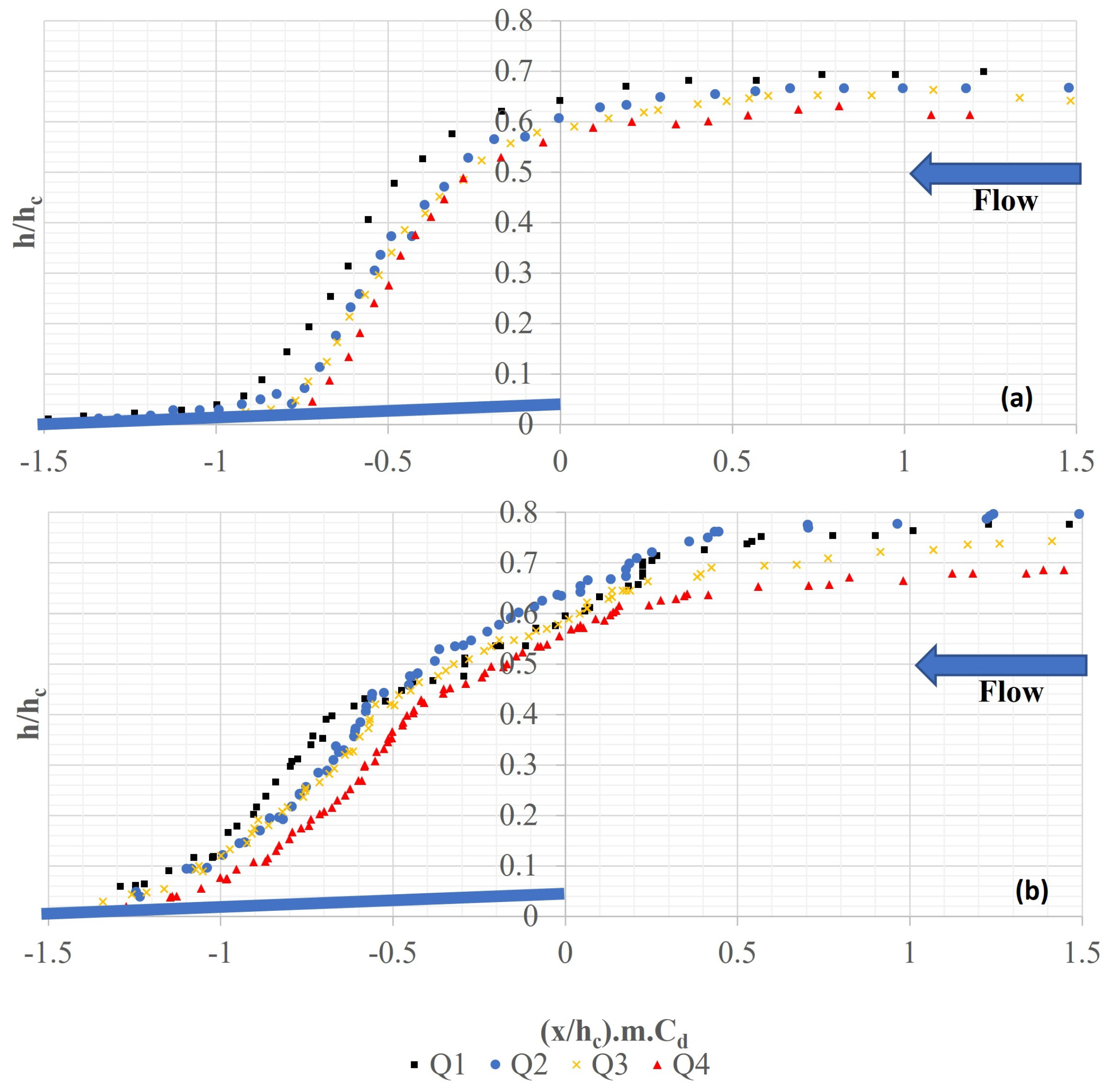
• According to the studies, the estimation of the flow rate coefficient ($C_d$), which is the design criterion, and accordingly the wet rack length, is the most important parameter that affects the flow rate entering the intake structure. Good calculation of this parameter will provide both economical solutions and optimum flow rate input.
• The turbulence models in flow separation have different behavior. In this study, the $k-\epsilon$ turbulence model and the $k-\Omega$-based Shear-Stress Transport (SST) model, which are the most widely used RANS turbulence models in the literature, were used. The results obtained with the tests are almost the same when considering the behavior of the flow curves and the total amount of water taken.
• In this study, different formulations were applied for rectangular bars. Regarding the coefficient of discharge, rectangular bars have been found to show larger maximum values than T-shaped bars in the literature, and thus, will require relatively shorter rack length.

This study examined the usability of 3D CFD modeling for old structures with complex and limited data, such as secondary intakes, and in this regard, the study’s recommendations may be useful for consulting companies dealing with similar issues. Considering the total simulation times for domains containing approximately the same number of elements and in the simulations with the same parallel computation, modeling with OpenFOAM yielded approximately 11% faster calculations. However, it should be noted that this advantage is increased by the availability of a “cold-start” simulation technique for OpenFOAM. The results are in agreement with the studies in the literature. The intake is expected to collect the same amount of water as clean water with an increase in the required wet rack length. As such, experiments with sediments are required to understand the behavior of the rack under these conditions. For future studies, different turbulence models should be tested, and the results should be compared.

References

1. Garot, F. De Watervang met liggend rooster. Ing. Ned. Indie 1939, 6, 115–132. [Google Scholar]
2. Bouvard, M. Debit d’une grille par en dessous. Houille Blanche 1953, 3, 290–291. [Google Scholar] [CrossRef]
3. Kuntzmann, J.; Bouvard, M. Theoretical study of bottom type water intake grids. Houille Blanche 1954, 40, 569–574. [Google Scholar] [CrossRef]
4. Noseda, G. Operation and design of bottom intake racks. In Proceedings of the VI General Meeting IAHR, The Hague, The Netherlands; 1955; Volume 3, pp. C17-1–C17-11. [Google Scholar]
5. Noseda, G. Correnti permanenti con portata progressivamente decrescente, defluenti su griglie di fondo. Energ. Elettr. 1 1956, 33, 41–51. [Google Scholar]
6. Noseda, G. Correnti permanenti con portata progressivamente decrescente, defluenti su griglie di fondo. Energ. Elettr. 6 1956, 33, 565–581. [Google Scholar]
7. Mostkow, M. Sur le calcul des grilles de prise d’eau. Houille Blanche 1957, 4, 569–576. [Google Scholar] [CrossRef]
8. Brunella, S.; Hager, W.; Minor, H.E. Hydraulics of Bottom Rack Intake. J. Hydraul. Eng. 2003, 129, 2–10. [Google Scholar] [CrossRef]
9. De Marchi, G. Profili Longitudinali della Superficie Libera delle Correnti Permanenti Lineari con Portata Progressivamente Crescente o Progressivamente Decrescente Entro Canali di Sezione Constante; Consiglio Nazionale Delle Ricerche: Rome, Italy, 1947; pp. 203–208. [Google Scholar]
10. Frank, J.; Von Obering, E. Hydraulische Untersuchungen für das Tiroler Wehr; Der Bauingenieur: Prague, Czech Republic, 1956; pp. 96–101. [Google Scholar]
11. Dagan, G. Notes sur le calcul hydraulique des grilles par-dessous. Houille Blanche 1963, 1, 59–65. [Google Scholar] [CrossRef]
12. García, B. Estudio Experimental y Numérico de los Sistemas de Captación de Fondo. Ph.D. Thesis, Escuela Internacional de Doctorado de la Universidad Politécnica de Cartagena, Universidad Politécnica de Cartagena, Cartagena, Spain, 2016. [Google Scholar]
13. Righetti, M.; Rigon, R.; Lanzoni, S. Indagine sperimentale del deflusso attraverso una griglia di fondo a barre longitudinali. In Proceedings of the XXVII Convegno di Idraulica e Costruzioni Idrauliche, Geneva, Italy, 12–15 September 2000; Volume 3, pp. 112–119. [Google Scholar]
14. Castillo, L.; Bermejo, J.T.G. Estudio Experimental y Numérico de los Sistemas de Captación de Fondo. Ph.D. Thesis, Universidad Politécnica de Cartagena Departamento de Ingeniería Civil, Cartagena, Spain, 2016. [Google Scholar]
15. Drobir, H. Entwurf von Wasserfassungen im Hochgebirge; Österreichische Wasserwirtschaft: Mondsee, Austria, 1981; pp. 243–253. [Google Scholar]
16. Stokkebø, O. Bekkeinntak på Kraftverkstunneler—Sluttrapport fra Bekkeinntakskomiteen; Vassdragsregulantenes Forening: Norway, 1986. [Google Scholar]
17. Bombardelli, F.A. Computational multi-phase fluid dynamics to address flows past hydraulic structures. In Proceedings of the Symposium on Hydraulic Structures, Porto, Portugal, 9–11 February 2012. [Google Scholar]
18. Blocken, B.; Gualtieri, C. Ten iterative steps for model development and evaluation applied to Computational Fluid Dynamics for Environmental Fluid Mechanics. J. Environ. Model. Softw. 2012, 33, 1–22. [Google Scholar] [CrossRef]
19. Castillo, L.G.; García, J.T.; Carrillo, J.M. Influence of Rack Slope and Approaching Conditions in Bottom Intake Systems. Water 2017, 9, 65. [Google Scholar] [CrossRef]
20. Carrillo, J.M.; García, J.T.; Castillo, L.G. Experimental and Numerical Modelling of Bottom Intake Racks with Circular Bars. Water 2018, 10, 605. [Google Scholar] [CrossRef]
21. Menter, F.R. Two-equation eddy-viscosity turbulence models for engineering applications. AIAA J. 1994, 32, 1598–1605. [Google Scholar] [CrossRef]
22. Launder, B.E.; Spalding, D.B. The numerical computation of turbulent flows. Comput. Methods Appl. Mech. Eng. 1974, 3, 269–289. [Google Scholar] [CrossRef]
23. Ansys Inc. ANSYS Fluent Workbench Totorial Guide. ANSYS2021. Available online: https://forum.ansys.com/uploads/846/SCJEU0NN8IHX.pdf (accessed on 20 February 2024).
24. Torres, C.; Borman, D.; Sleigh, A.; Neeve, D. Three dimensional numerical modelling of full-scale hydraulic structures. In Proceedings of the 37th IAHR World Congress, Kuala Lumpur, Malaysia, 13–18 August 2017; pp. 1335–1343. [Google Scholar]
25. García, J.T.; Castillo, L.G.; Haro, P.L.; Carrillo, J.M. Diseño de Sistemas de Captación de Fondo; Las Jornadas de Ingeniería del Agua (JIA): Coruña, Spain, 2017. (In Spanish) [Google Scholar]
26. Frank, J. Fortschritte in der Hydraulic des Sohlenrechens; Der Bauingenieur: Prague, Czech Republic, 1959; pp. 12–18. [Google Scholar]
27. Yilmaz, N.A. Hydraulic Characteristics of Tyrolean Weirs; Orta Doğu Teknik Üniversitesi: Ankara, Turkey, 2010. [Google Scholar]
28. Yildiz, A.; Marti, A.I.; Gogus, M. Numerical and experimental modelling of flow at Tyrolean weirs. Flow Meas. Instrum. 2021, 81, 102040. [Google Scholar] [CrossRef]
Figure 1. Downstream view of Stigansåni brook intake during (a) dry conditions and (b) wet conditions.
Water 16 00737 g001
Figure 2. (a) Fluid Domain. (b) Intake structure.
Water 16 00737 g002
Figure 3. The computational mesh used in the full-scale modeling using ANSYS Fluent.
Water 16 00737 g003
Figure 4. Boundary conditions used in the full-scale modeling using ANSYS Fluent.
Water 16 00737 g004
Figure 5. Defined computational and modelled structures for OpenFOAM simulations. Flow direction is from right to left.
Water 16 00737 g005
Figure 6. (a) Modelling domain with simplified surroundings of Stigansåni river intake (b) Modelling domain with measured topology. Intake structure is presented at the front with the weir inside.
Water 16 00737 g006
Figure 7. Generated grid with fine resolution that are applied in OpenFOAM. (a) Grid resolution at the domain from the top. (b) Grid resolution at the upstream end of the rack bars. (c) Grid resolution inside the intake with the weir.
Water 16 00737 g007
Figure 8. Variation of water volume fraction inside of the brook intake at (a) 300 s for ANSYS Fluent. (b) 100∼200 s for OpenFOAM simulations. (water level is  ( r α ) = 0.5 ) (The figure from ANSYS Fluent is taken the beginning side of the inclined rack, while the figure from OpenFOAM is taken the end side of the inclined rack).
Water 16 00737 g008
Figure 9. Flow profiles inside of the brook intake for different flow rates at 300 s with ANSYS Fluent.
Water 16 00737 g009
Figure 10. Flow profiles over the rack at 300 s with (a) ANSYS Fluent. (b) OpenFOAM.
Water 16 00737 g010
Figure 11. Dimensionless flow profiles over the rack (a) with ANSYS Fluent. (b) with OpenFOAM.
Water 16 00737 g011
Figure 12. Variation in overflow coefficient for Tyrolean weir.
Water 16 00737 g012
Figure 13. Change of Wetted Rack Length under different flow rates ([8,10,15,16]).
Water 16 00737 g013
Figure 14. Comparison of discharge coefficients obtained from variable expressions under different flow rates ([1,6,26]).
Water 16 00737 g014
Figure 15. Variation of the discharge coefficient along the rack for rectangular bars ( m = 0.429 ).
Water 16 00737 g015
Figure 16. Simulated flow rate over time at the intake outlet with (a) simplified surroundings and (b) with natural topology.
Water 16 00737 g016
Figure 17. Water capture capacity for the Stigansåni intake ( m = 0.429 ).
Water 16 00737 g017