Effects of Geometry on Artificial Tracer Dispersion in Synthetic Karst Conduit Networks

Abstract

This paper presents the modeling results of tracer test simulations performed using COMSOL Multiphysics (version 6.1), a powerful software for multiphysics simulation. The simulations consist of the propagation of artificial tracers injected into different model configurations. This study is based on computational fluid dynamics (CFDs), which allows us to take into consideration the turbulent regime of the water flow in conduits. The objective of this contribution is to identify the relationship between the tracer dynamics and the geometric parameters of synthetic karstic systems via a systematic investigation of the occurrence of dual-peaked breakthrough curves (BTCs) in tracer tests. Various conduit structures were proposed by modifying five key factors: conduit diameter, presence of pools, connection angle between conduits, distance of the outlet from the inlet, and number of branches. The next step will be to confront these computational experiments with real-world tracer test experiments.

1. Introduction

Karstic aquifers play a significant role in freshwater supply in many regions worldwide, but they are vulnerable to both contamination and overexploitation. Approximately 20% to 25% of the global population relies heavily or entirely on groundwater from karstic aquifers [1]. Their hydrogeological heterogeneity is related to highly permeable preferential flow paths formed by the dissolution of the surrounding rock [2,3]. In general, the karst aquifer consists of two main hydrogeological compartments: the matrix, which accounts for over 90% of the aquifer volume and plays a significant role in storage, and the conduits, which occupy a minimal volume but are responsible for fast flow generation, as they are responsible for approximately 90% of the total discharge in highly karstified aquifers [4]. Then, hydrogeologists generally conceptualize karst aquifers as dual systems consisting of fast-flowing groundwater concentrated within conduits included in a less permeable matrix. The location and size of the conduits generally remain unknown at the aquifer scale, which implies significant challenges to the potential application of physically distributed karst models [5,6]. The inability to directly evaluate and precisely ascertain the specific structure and positioning of conduits in the subsurface presents a significant obstacle to accurately characterizing and modeling the flow patterns in karst systems. Therefore, various methods have been developed to characterize groundwater drainage structures in such systems. One effective way is using artificial tracer tests, which have demonstrated their significance in studying the dynamics of conduit flow and solute transport, especially in highly karstified aquifers [7]. These challenges include modeling solute transport in karst conduits, assessing short-term variations in tracer test responses, and examining accidental pollution scenarios involving discharge variations during the infiltration and restitution of contaminants.

Artificial tracer tests are widely used in the field of hydrogeology as specialized methodologies for investigating flow-paths, flow dynamics, transport processes, and interactions between water and rocks. Solute transport is investigated in various hydrological situations, including low and high water levels, corresponding to “dry” and “rainy” periods. The primary objectives of these techniques include the exploration of interconnections between multiple locations in karstic watersheds related to travel time and residence time estimations, research into transport mechanisms, mixing and circulation processes, water–rock interactions, and the characterization of aquifer parameters, among other applications [8,9,10,11,12,13,14,15,16,17,18,19,20,21,22,23,24,25]. Artificial tracer tests are also dedicated to defining catchment boundaries or recharge areas, identifying pollution sources, or for identifying post-seismic modification on groundwater flow paths [26,27,28].

There are three main approaches in tracer test simulations based on numerical, laboratory, or field experimental methods. Numerous experimental studies have been conducted to better assess the relationship between karstic geometry and BTCs, shedding light on the complex dynamics of fluid flow in karstic systems [9,29,30,31,32,33]. Previous laboratory experiments based on the injection of conservative tracers in a pool-pipe system with variable pool placements, sizes, and numbers [34,35,36] have already investigated the relationship between conduit structures and BTCs, shedding light on the effect of pool volume on BTCs in karst conduits. However, the experimental results showed that pool position did not affect BTC, but higher pool sizes or a more significant number of pools increased BTC tailing and decreased peak concentration. A transfer function approach constitutes another way to characterize the residence time distribution curves obtained from fluorescent dye tracer tests [8,36]. This systematic approach comprehensively integrates all pertinent processes within a conceptual reservoir model. The proposed model comprises three delayed subfunctions, which account for the time delay in solute transport. This delay can be attributed to complex structures acting as dead zones and the associated friction effects [36,37,38].

In a recent study by Wang et al. [39], lab-scale experiments were conducted to investigate the solute transport process in dual-conduit structures examining how the dual-conduit structure affects the shape of BTCs. Three setups were constructed by varying the length ratio between the two conduits, the total length of the conduits for a specified length ratio, and the connection angle between the conduits. Results have shown that increasing the length ratio between the two conduits resulted in greater separation between the BTC peaks. Additionally, the concentration value of the first peak increased while the concentration value of the second peak decreased. Increasing the total length of the conduits also led to a higher delay between the two peaks. Finally, modifying the connection angle between the two conduits affected the sizes of the peaks. Specifically, increasing the first angle and decreasing the second one resulted in a smaller size for the first peak, indicating a reduced mass transported through the shorter conduit. In contrast, the size of the second peak increased, suggesting an increased mass transported through the longer conduit. However, the study has some limitations. The experiments were conducted in a lab-scale setting using idealized dual-conduit structure models, which may not fully represent the complex conditions of natural karst aquifers. Additionally, the study focused on the influence of conduit geometry on BTCs and did not consider other factors that may affect solute transport in karst aquifers.

The objective of this contribution is to propose a parametric study through simulations of artificial tracer tests using COMSOL Multiphysics. The numerical simulations focus on the influence of the geometric parameters of the system, such as conduit lengths, connection angles, conduit diameters, pool size, and exchange between matrix and conduits. That allows improvements in the comprehensive analysis of the relationship between the input parameters and the resulting tracer breakthrough curves, residence time distribution estimations, or other relevant output variables.

2. Materials and Methods

2.1. COMSOL Multiphysics^®

COMSOL Multiphysics (version 6.1), a finite element-based simulation software, offers various predefined interfaces, including computational fluid dynamics (CFDs). It has gained considerable recognition in environmental applications in recent years. COMSOL Multiphysics is a simulation platform that allows researchers and engineers to model complex systems. By providing an easy-to-use environment for virtual experimentation, it facilitates high-speed calculations. The COMSOL material library offers an extensive array of features that integrate multiphysics phenomena that allow researchers to explore the intricate interactions of multiple physical domains in one comprehensive study. Moreover, the model library implements prebuilt models and templates that can streamline the simulation setup process.

The CFD Module, an optional package within COMSOL Multiphysics, enhances the software’s capabilities by providing customized physics interfaces and specialized functionality for analyzing fluid flow in all its forms.

2.2. Physical Interfaces

2.2.1. Turbulent Flow

In karst conduits, if one considers a mean diameter of 1 m and a mean flow velocity of 0.1 ms⁻¹ mostly characteristic of a low-flow period, a minimum Reynolds number of 10,000 can be estimated. Therefore, we obviously choose to operate in turbulent flow regimes [40,41]. The incorporation of turbulence equations aims to capture the intricate flow characteristics and complexities inherent in high-Reynolds-number scenarios, providing a more comprehensive understanding of the tracer test behavior in several karst conduits geometries. The CFD module within COMSOL Multiphysics incorporates the single-phase flow branch, which consists of various subbranches with physics interfaces. The turbulent flow k–ε interface appears as the more relevant, since it is designed to simulate single-phase flows at elevated Reynolds numbers. It allows a numerical resolution of the Reynolds-averaged Navier–Stokes (RANS) equations coupled to the continuity equation to ensure mass conservation. The model introduces two additional transport equations and two dependent variables: the turbulent kinetic energy, k, and the turbulent dissipation rate, ε. In turbulent flow, the Navier–Stokes equation maintains its identity with the laminar counterpart, yet an additional component emerges in the transport equation [42]. Equation (1) represents the transport equation for k, where Pk is the production term presented in Equation (2). The transport equation for ε is shown in Equation (3).

$$\rho \frac{\partial k}{\partial t}+\rho u . \mathsf{\nabla }k=\mathsf{\nabla } \left(\left(\mu +\frac{{\mu }^T}{\sigma k}\right) \mathsf{\nabla }k\right)+Pk-\rho \epsilon$$

(1)

$$P_K={\mu }_T\left(\mathsf{\nabla }u \left(\mathsf{\nabla }u+{\left(\mathsf{\nabla }u\right)}^T\right)-\frac{2}{3}{\left(\mathsf{\nabla }.u\right)}^2\right)-\frac{2}{3} \rho k \mathsf{\nabla }u$$

(2)

$$\rho \frac{\partial \epsilon }{\partial t}+\rho u . \mathsf{\nabla }\epsilon =\mathsf{\nabla } \left(\left(\mu +\frac{{\mu }^T}{\sigma \epsilon }\right)\mathsf{\nabla }\epsilon \right)+C{\epsilon }_1 \frac{\epsilon }{k} Pk-C{\epsilon }_{2 }\rho \frac{{\epsilon }^2}{k}$$

(3)

where μ^T represents the turbulent viscosity shown in Equation (4) and C_μ is a model constant.

$${\mu }_T=\rho C_{\mu }\frac{k^2}{\epsilon },$$

(4)

The model constants in Equations (1)–(4) are summed up in

Table 1. Values of the parameters of the k epsilon turbulence model, which is a widely used approach in computational fluid dynamics (CFDs) to simulate turbulent flows by solving transport equations for turbulence kinetic energy and its dissipation rate.

Constant	Value
Cμ	0.09
Cε1	1.44
Cε2	1.92
σk	1.0
σε	1.3

.

2.2.2. Transport of Diluted Species (TDS)

The TDS (transport of diluted species) interface, located within the chemical species transport branch, computes the concentration distribution of a diluted solute in a solvent. This interface considers various transport mechanisms, including diffusion based on Fick’s law and convection when coupled with a flow field. Considering these driving forces, the TDS interface allows for accurately calculating solute concentration profiles in a given system. Using the transport of diluted species interface, we solve the initial concentration of the model, which follows a Gaussian distribution. Equation (5) represents the transport of a species in a fluid. It describes the change in concentration (c) concerning time (t) and includes terms related to advection (u∇ci) and flux divergence (u∇Ji). The advection term accounts for the transport of the species due to the fluid velocity (u), while the flux divergence term represents the spatial variation of the species flux (ji) in the direction of the velocity vector. Ri represents any additional contributions to the species concentration, such as chemical reactions or external sources. Equation (6) represents the flux of a species in a fluid. It relates the flux (Ji) to the concentration gradient (∇ci) through the diffusion coefficient (Di). The negative sign indicates that the species flows from regions of higher concentration to regions of lower concentration, following the concentration gradient.

$$\frac{\partial c}{\partial t}+u\cdot \mathsf{\nabla }ci+u\cdot \mathsf{\nabla }Ji=Ri$$

(5)

$$Ji=-Di \mathsf{\nabla } Ci$$

(6)

2.3. Case Studies

The methodology of this study focuses on investigating the influence of synthetic conduit geometry characterized by the presence of mixing zones but also of networks of conduits with different connections on TDS function statistics [43].

Numerical experiments were conducted based on idealized pool-conduit structure models with a fixed diameter of 2 m under turbulent flow conditions. This pool-conduit structure comprises three distinct sections: the inlet, the conduit-pool system, and the outlet. The inflow velocity was set at 0.1 ms⁻¹, which aligns with field velocities within a realistic field range. The concentration at the inflow is estimated by Equation (7)

$$C\left(t\right)=\frac{1}{\sigma \sqrt{2\pi }} e^{-\frac{1}{2} {\left(\frac{t-\mathsf{\mu }}{\sigma }\right)}^2}. C_0$$

(7)

where t represents time, C₀ is the initial concentration established at 1 mol/m³, and $\sigma$ and $\mathsf{\mu }$ represent the mean and standard deviation of the distribution.

The investigation consists of six cases (

Table 2. Presentation of the different geometries considered in CFD simulation affecting BTCs within complex karst conduit systems. Each case investigates specific aspects: Case 1: variable inlet-outlet distance/Cases 2–3: impact of pool characteristics (size and position)/Case 4: conduit diameter/Case 5: connection angles between conduits/Case 6: number of branches from 1 up to 3. They correspond to the main geometries already identified in karst networks on a large scale [11] that can be of interest in artificial tracer dispersion discussion.

Cases	Conditions	Parameters	Illustration
Case 1	Distance of the outlet from the inlet (D0 = Dconduit = 2 m)	L = L0 L = 10 m L = 20 m
Case 2	Size of pools (D0 = Dconduit = 2 m and LPO = 2 m)	LP = 2×PO LP = 3×LPO LP= 4×LPO LP= 5×LPO
Case 3	Position of pools (Cubic Pools 6 × 6 m and L’O = 2 m)	L’ = 2 × L’O L’ = 2 × L’O L’ = 3 × L’O
Case 4	Diameter of conduits	D = 2 × D0 D = 3 × D0 D = 4 × D0 D = 5 × D0
Case 5	Angle of connection (D0 = Dconduit = 2 m)	Alpha α α= 10…90
Case 6	Numbers of branches	N = 1, 2, 3

), each focusing on different factors influencing solute transport in karst conduits. The inlets are considered points of entry for the solute, allowing controlled injection into the system. The outlets are considered exit points, where the solute was monitored and sampled to measure its concentration and behavior. Cavities within the conduit system added complexity to the flow and transport processes as they introduced additional pathways and zones of interaction. The reservoir’s characteristics, such as its size, shape, and connectivity, significantly impact the movement of water and the formation of karst features. This affects the flow paths, velocity, and direction of groundwater, influencing the distribution of dissolved substances and the development of features like springs, caves, and underground rivers. The reservoir refers to a storage space for water, which can accumulate during periods of precipitation. It plays a crucial role in the storage and movement of water within the system [44,45,46].

The different geometries considered in this contribution are shown in Table 2. They correspond to the main geometries already identified in karst networks on a large scale [11] that can be of interest in artificial tracer dispersion discussion. The first case examines the variation in distance of the outlet from the inlet and refers to changes in the spatial separation between the points where water enters the system (inlet) and the point where it exits (outlet). This distance variation is particularly relevant in studying how water travels through underground karst formations, characterized by complex networks of conduits, caves, and fractures. The second case considers the influence of pools within the conduit system, considering both their size and position. Additionally, the diameter of a single conduit is analyzed in the third case to study its influence on the output signal of BTCs. Furthermore, the investigation examines the angle connection between the conduits in case four. This can provide insights into the effect of solute dispersion and mixing. Case five concerns the influence of connection angle in the exchange of solutes between the conduits, potentially affecting the overall solute transport within the system. Case six refers to the number of branches. The number of branches within this network can impact critical aspects such as flow distribution, dispersion, and mixing.

2.4. Residence Time Distribution

The tracer test involves injecting a conservative tracer into an unknown system to assess the transit time or response of the system. To comprehend the mixing conditions within the complex system, it is essential to determine the residence times of each volume element within the system. When a tracer is introduced instantaneously, its components exit the system at various intervals. These intervals are calculated by observing fluctuations in tracer concentration at the system outlet or other specific points within the system [7]. Mathematically, if a tracer mass M is added at a time t = 0 s, its concentration at the outlet, denoted as c(t), can be expressed as a function of time involving the spring flow function Q(t) (Equation (8)). This brings us to the residence time distribution (RTD) concept, denoted as E(t), which can be estimated by integrating the product of concentration and flow functions (Equation (9)). This concept encapsulates the system’s behavior over time. The critical parameters derived from the RTD function include the mean residence time θ (Equation (10), calculated by integrating the product of time and the RTD function. This parameter offers insights into the average time a substance spends within the system. The analysis of RTD contributes to the understanding of fluid behavior, facilitating enhanced management and comprehension of dynamic systems [7].

$$M={{\displaystyle \int }}_{t=0}^{t=\infty }c\left(t\right)Q\left(t\right)dt,$$

(8)

$$E\left(t\right)=\frac{c\left(t\right)Q\left(t\right)}{{{\displaystyle \int }}_{t=0}^{t=\infty }c\left(t\right)Q\left(t\right)dt}\mathrm{Where} {{\displaystyle \int }}_{t=0}^{t=\infty }E\left(t\right)dt=1,$$

(9)

$$\theta ={{\displaystyle \int }}_{t=0}^{t=\infty }t E\left(t\right)dt,$$

(10)

The RTD function is a fundamental parameter to understand the behavior of solute transport within the system. By normalizing the concentration values, the RTD function allows one to focus on the temporal aspects of solute movement without being influenced by the absolute concentration values. The extracted parameters from the output signal include the following elements: the value of RTD, the peak time, and the arrival time (

Table 3. Description of the main parameters of the output signal.

Notations	Definitions	Units
RTD	Distribution of the time that solutes spend within the system	[s−1]
Tpeak	Elapsed time to peak concentration	[s]
Tarrival	Elapsed time to solute last detected	[s]

).

3. Results and Discussions

3.1. Simulation Results Using COMSOL Multiphysics

3.1.1. Case 1: Influence of the Distance of the Outlet from the Inlet

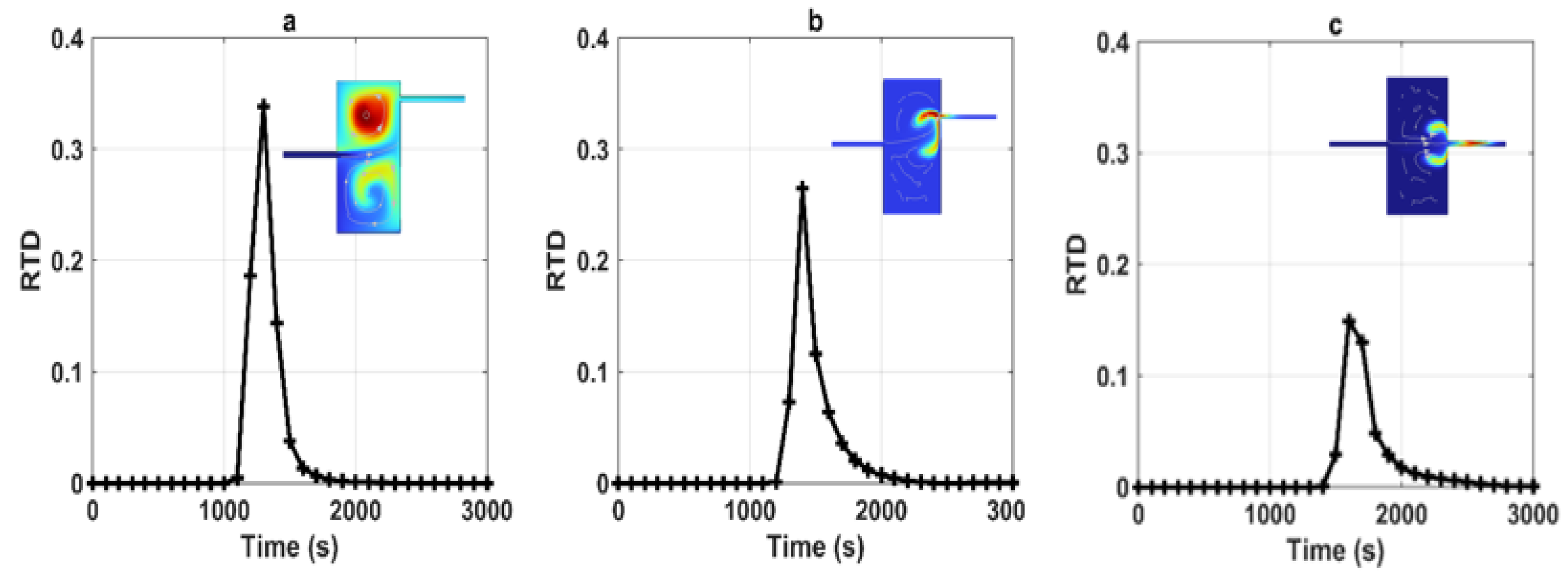
Through our observations (Figure 1,

Table 4. Statistical parameters from RTDs for the first case (variation of inlet–outlet distance).

Distance	Max Value of RTD (s−1)	Peak Time (s)	Arrival Time (s)
L = 20 m (a)	0.338	1600	2900
L = 10 m up (b)	0.265	1400	2300
L = 0 m up (c)	0.149	1300	2000

), as the distance decreases from 20 to 0 m, the RTD maximum value undergoes a gradual decrease from 0.338 to 0.149 s. Additionally, we noted a slight delay in the arrival time of the first peak, indicated by the time shift from t(a) = 1600 s to t(c) = 1300 s. Furthermore, the arrival time of the solute is similarly delayed from 2000 s to 2900 s while increasing the distance. This behavior can be attributed to the travel dynamics within the karstic conduit system. When the outlet is positioned closer to the inlet, solutes experience a relatively shorter travel distance and time. This configuration leads to less dispersion and more direct transport, subsequently contributing to a lower RTD value (as observed in case “c”) due to the shorter residence times; conversely, when the outlet is located farther from the inlet, solutes are afforded a longer travel path and increased interaction with conduit walls, other solutes, and fluid flow patterns. This dispersion and mixing result in an increase in the RTD value (as in case “a”), as solutes spend more time within the system. Additionally, we explored the influence of symmetry by inversely changing the up-and-down arrangement while maintaining the same distance difference. We observed that such symmetry changes did not significantly affect the extracted parameters.

3.1.2. Case 2: Influence of the Size of Pools

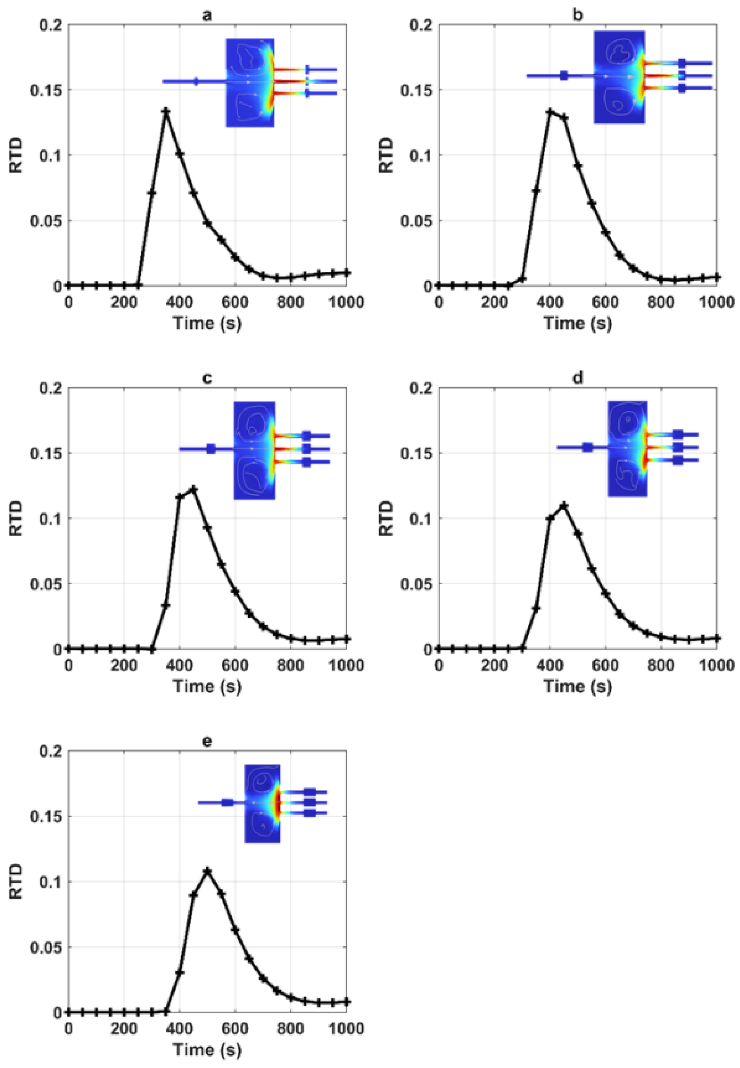
For this case, we examined how variations in pool size affect RTDs through a series of five numerical simulations (Figure 2 and

Table 5. Statistical parameters from RTDs for the second case (variation of the size of pools).

Lp	Max Value of RTD (s−1)	Peak Time (s)	Arrival Time (s)
Lp = 2 m (a)	0.110	400	800
Lp = 4 m (b)	0.113	450	820
Lp = 6 m (c)	0.125	500	820
Lp = 8 m (d)	0.117	500	820
Lp = 10 m (e)	0.113	500	820

). The various simulations demonstrated that there was no significant distinction observed. When the size of the pools increases, the max RTD value tends to increase slightly (Figure 2b,c). Larger pools provide more space for solutes to mix and interact with the surrounding water. This increased mixing leads to greater dispersion of solutes, causing them to spend more time within the system. As a result, the maximum value of the RTD function increases, indicating a more extended distribution of residence times. As well as the peak time, the value tends to increase slightly from 400 s (Figure 2a) to 500 s (Figure 2c–e). Furthermore, the time of arrival of the solute does not significantly change (t = 800–820 s). In this respect, the influence of the pool position on the exit signal appears negligible.

3.1.3. Case 3: Influence of the Position of Pools

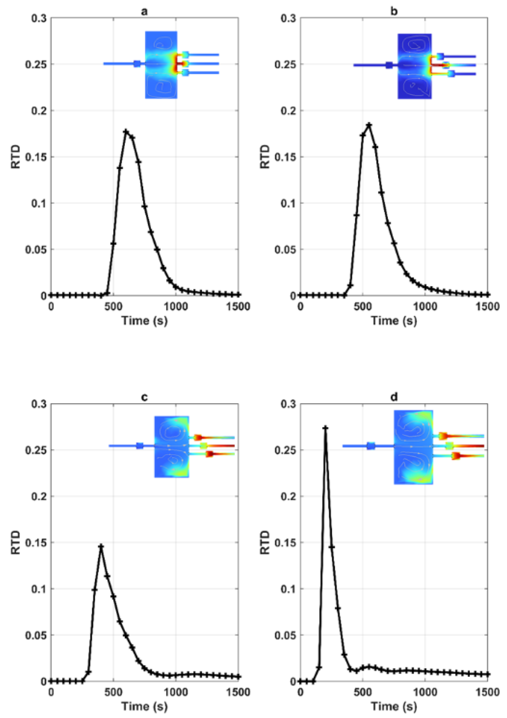
Comparing the RTDs shown in Figure 3, numerical results indicate that the pool position has little effect on the RTDs. The morphology of the curves appears similar for the exit signals (

Table 6. Statistical parameters from RTDs for the third case (variation in the position of the pools).

Lp	Max Value of RTD (s−1)	Peak Time (s)	Arrival Time (s)
L-L-L-L (a)	0.135	650	1200
L-L-2L-3L (b)	0.143	600	1300
2L-L-2L-3L (c)	0.187	500	1300
3L-L-2L-3L (c)	0.255	250	1400

). When the distance of the pools from the outlet increases, the RTD value tends to increase from RTD = 0.135 s (a) to 0.255 s (d). The arrival time increases from t = 1200 s to 1400 s. Then, a greater distance allows for decreased dispersion and mixing of solutes through the conduits.

3.1.4. Case 4: Influence of the Diameter of Conduits

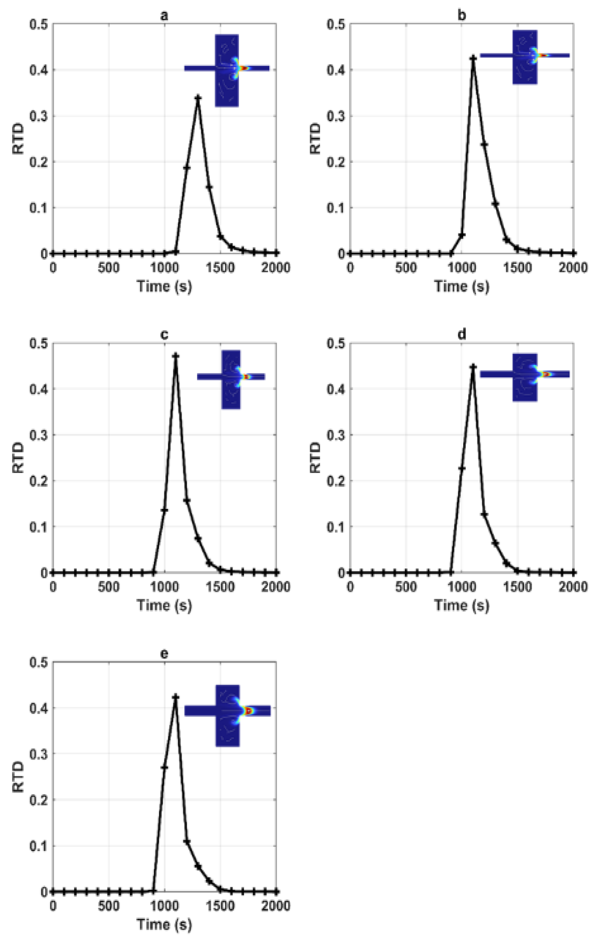
This case allows identifying the influence of the diameter of the conduits in the RTD functions (Figure 4,

Table 7. Statistical parameters from RTDs for the fourth case (variation in the diameters).

D	Max Value of RTD (s−1)	Peak Time (s)	Arrival Time (s)
D = 2 m (a)	0.338	1300	2000
D = 4 m (b)	0.424	1100	1800
D = 6 m (c)	0.471	1100	1800
D = 8 m (d)	0.447	1100	1600
D = 10 m (e)	0.423	1100	1600

). First, we can observe similarities in the morphology of the RTDs. The RTD peak values tend to increase from 0.338 s⁻¹ for D = 2 m to 0.471 s⁻¹ for D = 6 m. Then, the RTD maximum value slightly decreases. This increased flow velocity can result in faster solute transport through the system. As solutes spend less time within the conduits before exiting, the RTD maximum value tends to decrease.

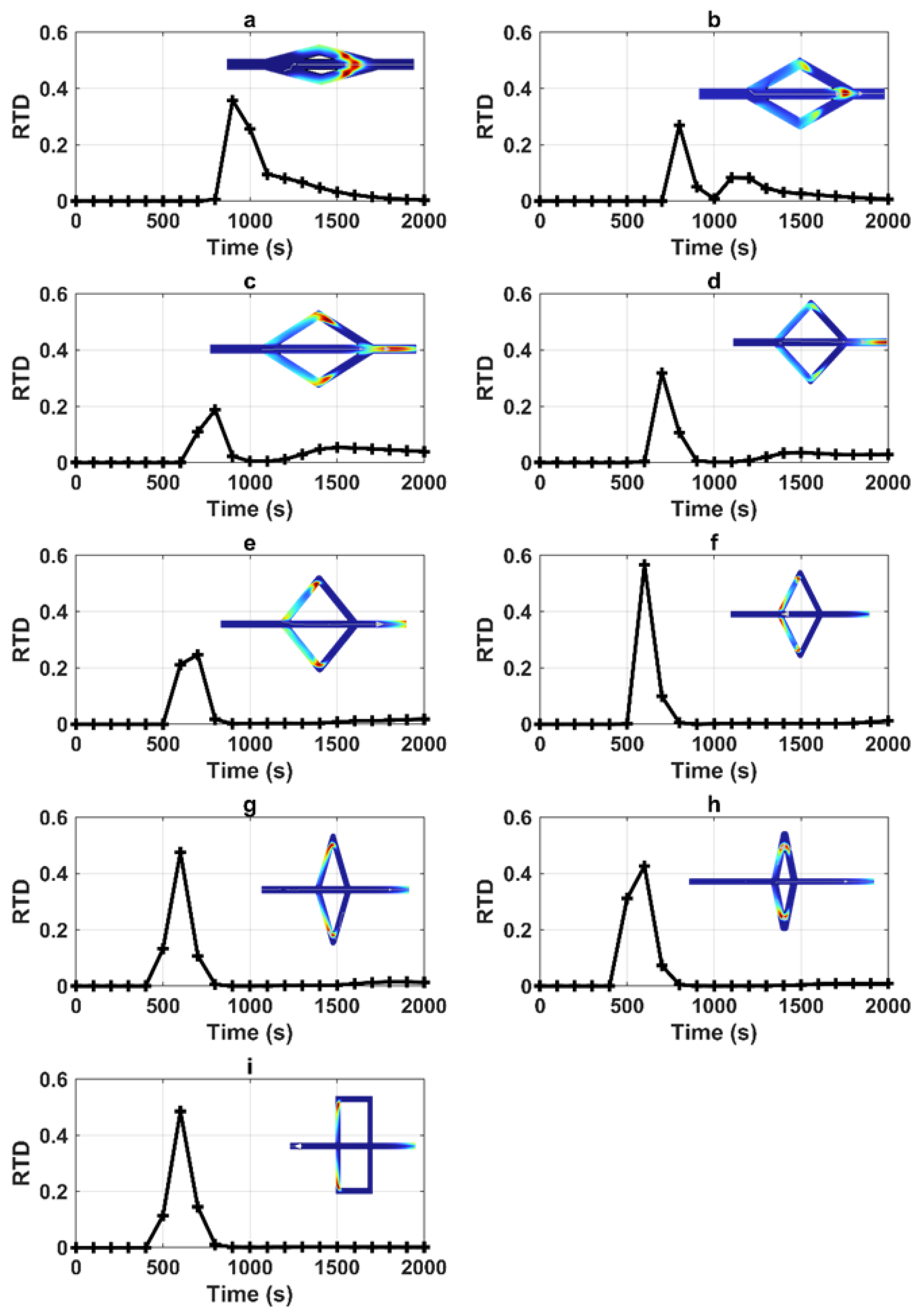
3.1.5. Case 5: Influence of the Angle of Connection

The influence of the connection angle between two conduits is shown in Figure 5 and

Table 8. Statistical parameters from RTDs for the fifth case (variation in the angle of connection).

Alpha		Max Value of RTD (s−1)	Peak Time (s)	Arrival Time (s)
Alpha 10 (a)	First peak	0.358	900	1900
	Second peak	0.066	1150	1900
Alpha 20 (b)	First peak	0.269	800	2000
	Second peak	0.081	1200	2000
Alpha 30 (c)	First peak	0.187	800	2200
	Second peak	0.053	1500	2200
Alpha 40 (d)	First peak	0.319	1100	2100
	Second peak	0.0359	1500	2100
Alpha 50 (e)	First peak	0.25	700	1400
	Second peak	-	-	1400
Alpha 60 (f)	First peak	0.567	600	900
	Second peak	-	-	900
Alpha 70 (g)	First peak	0.476	600	900
	Second peak	-	-	900
Alpha 80 (h)	First peak	0.427	600	900
	Second peak	-	-	900
Alpha 90 (I)	First peak	0.425	600	900
	Second peak	-	-	900

. The RTD functions exhibit a double peak for alpha =10–20–30 and 40 (Figure 5a–c,e). The RTD value of the first and second peaks fluctuates between the different simulations. The solute particles can rush through the conduits, resulting in an initial breakthrough peak and a secondary rise originating from the slower flow. As such, the complexity related to the connection angle between conduits appears as a determinant in the occurrence of the inversion of the peak maximum values. We can also observe that the arrival time of the first peak decreases from 900 s to 600 s. Effectively, as the connection angle increases, the first peak appears sooner while the second peak is delayed. This highlights the importance of considering the geometric arrangement of conduits when studying solute transport within karstic systems. In this respect, the angle of connection of the conduit appears as a determinant parameter of the RTD function variability.

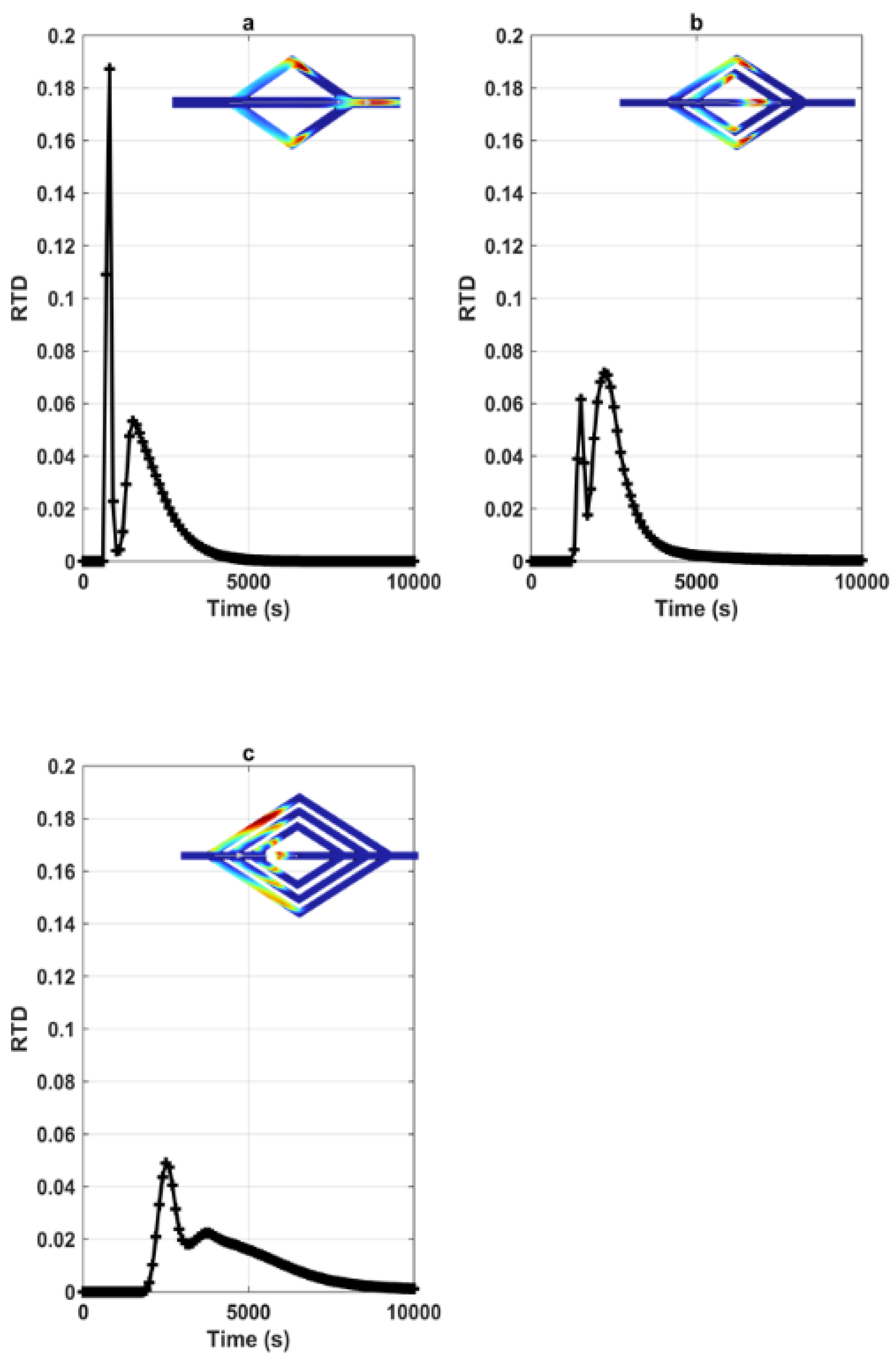
3.1.6. Case 6: Influence of the Number of Branches

The investigation into the influence of the number of branches of conduits on RTD signals provides a revealing comparison of how the structural complexity of the conduit network affects solute transport (Figure 6 and

Table 9. Statistical parameters from RTDs for the final case (variation in the number of branches for alpha = 30).

Alpha 30		Max Value of RTD (s−1)	Peak Time (s)	Arrival Time (s)
a	First peak	0.187	800	5200
	Second peak	0.52	1600	5200
b	First peak	0.616	1500	8000
	Second peak	0.709	2300	8000
c	First peak	0.474	2600	10,000
	Second peak	0.232	3800	10,000

). Concerning the first peak, the RTD values exhibit an increase for structures with two branches, followed by a decrease for structures with three branches. A similar trend is observed for the second peak. Additionally, both peak times are delayed. Moreover, the arrival time also increased, transitioning from t = 5200 s to t = 10,000 s as the number of branches increased from one to three.

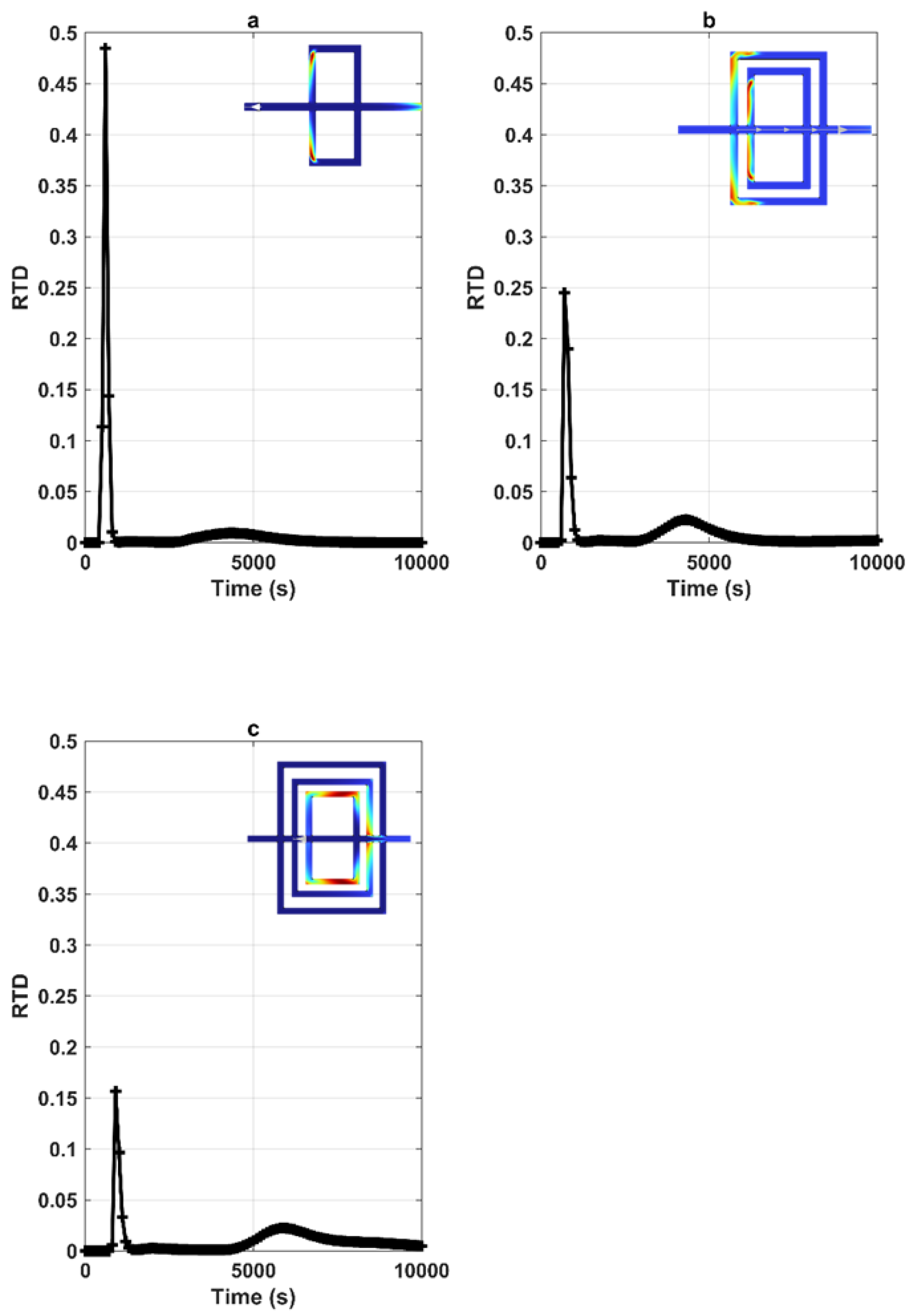
We also simulate the solute dispersion in synthetic karst conduits based on different numbers of branches for an angle of connection of 90 degrees (Figure 7,

Table 10. Statistical parameters from RTDs for the final case (variation in the number of branches for alpha = 90).

Alpha 90		Max Value of RTD (s−1)	Peak Time (s)	Arrival Time (s)
a	First peak	0.485	600	7100
	Second peak	0.009	4400	7100
b	First peak	0.245	700	8000
	Second peak	0.025	4700	8000
c	First peak	0.157	900	10,000
	Second peak	0.022	5900	10,000

). We show that the RTD maximum values decrease for a higher number of branches. A similar global trend is observed for the second peak. Additionally, both peak times are delayed. Moreover, the arrival time is delayed from 7100 s to 10,000 s. The interactions between branches can explain these modifications. The increase in the number of branches implies that solute particles can follow diverse pathways through the system, experiencing different flow velocities, directions, and different turbulence levels. The variations in flow pathways can lead to fluctuations in residence times and RTD values. With more pathways available, solute particles may encounter longer travel distances.

4. Discussion

Numerical simulations allow investigations into the dynamics of solute transport within synthetic karstic systems under various geometries. Our findings highlight the specific influence of parameters such as distance, pool size, conduit diameter, connection angles, and the number of branches on the RTD function. Our observations revealed that as the distance between the inlet and outlet of the karstic system decreases, the RTD peak values tend to decrease as well. This behavior can be attributed to the reduced dispersion effect, resulting in more advective-driven transport. We also found that symmetry changes had no effect on the RTD function.

The investigation of the impact of pool size and position on BTCs within karstic conduits has yielded insights into solute transport dynamics. In our study, we systematically explored these factors through a series of numerical simulations, revealing how variations in pool size and position affect the RTD values and other critical parameters. Our findings offer a nuanced perspective on the relationship between pool size and RTD function. Interestingly, we observed that as the size of the pools increased, the maximum RTD value showed a slight but noteworthy increase. This increase in RTD maximum is attributed to the larger pool sizes, which provide more space for solutes to mix and interact with the surrounding water. Consequently, this heightened mixing leads to greater dispersion of solutes, resulting in extended residence times within the system. Moreover, the peak time also exhibited a minor increase. Our numerical results are in accordance with the laboratory-scale experiments of Zhao et al. [39,40,41].

In addition to the impact of pool size, we explored the effect of pool position on BTCs. Our numerical results indicated that the position of the pools had little influence on the RTDs. The morphology of the RTD curves remained significantly similar for the exit signals, regardless of the pool’s placement. This can be attributed to the influence of distance on solute dispersion and mixing within the conduits. As the pools are positioned farther from the outlet, greater distance affords more opportunity for dispersion and mixing to occur, resulting in an increase in the RTD value. This effect contributed to an earlier arrival of the peak. On the other hand, larger pools, despite influencing RTD values, did not significantly alter the arrival time of solutes, which remained relatively constant. Furthermore, we examined how conduit diameter affects solute transport. The RTD values initially increased with larger conduit diameters before decreasing. This unexpected behavior was attributed to increased flow velocity, resulting in faster solute transport and reduced residence times. The connection angle between conduits also played a significant role in solute transport. Varying angles led to multi-peaked BTCs, with the first peak arriving earlier and the second peak delayed as the angle increased.

The next step will be to use the COMSOL simulations on more complex geometries, including, for example, fractal geometries in order to propose more insightful analyses of the BTC statistical parameters function of karst system geometry.

While these simulations have provided valuable insights into the behavior of the system under different conditions, it is important to mention the limitations of this study. This contribution mainly focuses on solute transport in the conduit under turbulent conditions without conduit-matrix exchange. Here, the matrix was considered impermeable, whereas the permeability of rocks can interact with the tracer transfer. Furthermore, our study is limited to 2D geometry. To explore these complex systems, 3D geometries with fracture would be more representative, but lead to extensive calculation times and parameterization.

However, we demonstrate that the field of numerical simulations offers a wide range of applications to analyze complex phenomena such as tracer test experiments in karst systems. To develop this study further, several improvements can be made. Firstly, conducting field-scale simulations on specific parts of real karst systems would provide more realistic results and insights into solute transport processes. Real-world conditions, such as heterogeneity, pools, or multiple flow paths along conduits, and the interactions between conduits and the surrounding rock matrix, may affect solute transport differently from that observed in the laboratory or in the numerical simulations. There is an increasing demand for integrating numerical methods to complement experimental studies in the solute transport field in karstic aquifers. This integration allows for exploring a more comprehensive range of conditions and manipulating parameters that may not be readily achievable through laboratory experiments alone. Combining field experimental studies with numerical approaches should provide a comprehensive and integrated approach to advancing our understanding of solute transport in karstic systems.

5. Conclusions

In this study, we examine the solute transport process in conduit-pool structures designed to reproduce an idealized karstic system. The main contributions of this study can be summarized as follows. We introduced the COMSOL Multiphysics dynamics model to interpret the BTCs. We have studied how the variation of several geometric factors can influence BTC shapes. First, we observed that as the distance from the inlet to the outlet increases, there are distinct effects on the BTCs. Our investigation into the impact of varying distances between inlet and outlet points within the karstic conduit system revealed a clear relationship between distance and RTD maximum values. Specifically, as the distance diminishes from 20 to 0 m, the RTD values progressively decrease from 0.338 to 0.149 s⁻¹. Second, numerical results show that the pool size and position have no significant effect on the BTCs, consistent with previous studies. Third, conduit diameter variation depicts an effect on RTD values and on the arrival time of solute. The RTD maximum values tend to increase first and then decrease. Finally, we have examined the influence of the connection angle and the number of branches. Results show that the connection angle between two conduits has an essential impact on the transport process, with a significant impact on RTD maximum values, arrival time, and the occurrence of multi-peaked BTCs. Furthermore, the variation in the number of branches compares how the conduit network’s structural complexity affects solute transport within the karstic system.

References

- Ford, D.C.; Williams, P.W. Karst Geomorphology and Hydrology. J. Geol. 1991, 98, 797–798. [Google Scholar]
- Bakalowicz, M. Karst groundwater: A challenge for new resources. Hydrogeol. J. 2005, 13, 148–160. [Google Scholar] [CrossRef]
- Jourde, H.; Wang, X. Advances, challenges, and perspective in modeling the functioning of karst systems: A review. Environ. Earth Sci. 2023, 82, 396. [Google Scholar] [CrossRef]
- Chang, Y.; Wu, J.C.; Jiang, G.H.; Nan, T.C.; Xie, Y.F. Effect of different conduit network recharge ways on karst spring simulation. J. Hydrol. Eng. 2019, 24, 04019038. [Google Scholar] [CrossRef]
- Borghi, A.; Renard, P.; Cornaton, F. Can one identify karst conduit networks geometry and properties from hydraulic and tracer test data. Adv. Water Resour. 2016, 90, 99–115. [Google Scholar] [CrossRef]
- Goldscheider, N.; Drew, D. Methods in Karst Hydrogeology; CRC Press: Boca Raton, FL, USA, 2016. [Google Scholar]
- Labat, D.; Mangin, A. Transfer function approach for artificial tracer test interpretation in karstic systems. J. Hydrol. 2015, 529, 866–871. [Google Scholar] [CrossRef]
- Benischke, R. Review: Advances in the methodology and application of tracing in karst aquifers. Hydrogeol. J. 2021, 29, 67–88. [Google Scholar] [CrossRef]
- Goldscheider, N.; Neiman, J.; Pronk, M.; Smart, C. Tracer Tests in Karst Hydrogeology and Speleology. Int. J. Speleol. 2008, 37, 27–40. [Google Scholar] [CrossRef]
- Alireza, N.; Mohammadi, Z. Comparison of the results of pumping and tracer tests in karst terrain. J. Cave Karst Stud. Natl. Speleol. Soc. Bull. 2016, 78, 110–118. [Google Scholar]
- Jihong, Q.; Xu, M.; Cen, X.; Wang, L.; Zhang, Q. Characterization of Karst Conduit Network Using Long-Distance Tracer Test in Lijiang, Southwestern China. Water 2018, 10, 949. [Google Scholar]
- Metka, P. The Use of Artificial Tracer Tests in the Process of Management of Karst Water Resources in Slovenia. In Handbook of Environmental Chemistry; Springer: Berlin/Heidelberg, Germany, 2019; pp. 133–156. [Google Scholar]
- Bodin, J.; Porel, G.; Nauleau, B.; Paquet, D. Delineation of discrete conduit networks in karst aquifers via combined analysis of tracer tests and geophysical data. Hydrol. Earth Syst. Sci. 2022, 26, 1713–1726. [Google Scholar] [CrossRef]
- Martín-Rodríguez, J.; Mudarra, M.; De la Torre, B.; Andreo, B. Combining Quantitative Analysis Tools (Cross-Correlation Analysis and Dye Tracer Tests) to Assess Response Times in Karst Aquifers. The Ubrique Karst System (Southern Spain). In Advances in Karst Sciences Eurokarst Malaga; Springer: Berlin/Heidelberg, Germany, 2022; pp. 41–47. [Google Scholar]
- Metka, P.; Kogovšek, J. Identifying the characteristics of groundwater flow in the Classical Karst area (Slovenia/Italy) by means of tracer tests. Environ. Earth Sci. 2016, 75, 1446. [Google Scholar]
- Richter, D.; Goeppert, N.; Goldscheider, N. New insights into particle transport in karst conduits using comparative tracer tests with natural sediments and solutes during low-flow and high-flow conditions. Hydrol. Process. 2022, 36, e14472. [Google Scholar] [CrossRef]
- Kogovšek, J.; Metka, P. Solute transport processes in a karst vadose zone characterized by long-term tracer tests (the cave system of Postojnska Jama, Slovenia). J. Hydrol. 2014, 519, 1205–1213. [Google Scholar] [CrossRef]
- Assunção, P.; Galvão, P.; Lucon, T.; Doi, B.; Marshall Fleming, P.; Marques, T.; Costa, F. Hydrodynamic and Hydrodispersive Behavior of a Highly Karstified Neoproterozoic Hydrosystem Indicated by Tracer Tests and Modeling Approach. J. Hydrol. 2023, 619, 129300. [Google Scholar] [CrossRef]
- Xinyu, C.; Xu, M.; Qi, J.; Zhang, Q.; Shi, H. Characterization of karst conduits by tracer tests for an artificial recharge. Hydrogeol. J. 2016, 29, 2381–2396. [Google Scholar]
- Werner, A.; Hötzl, H.; Maloszewski, P.; Werner, S.S. Interpretation of Tracer Tests in Karst Systems with Unsteady Flow Conditions; IAHS Publications: Wallingford, UK, 1998; Volume 247, pp. 15–26. [Google Scholar]
- Sivelle, V.; Labat, D.; Duran, L.; Fournier, M.; Massei, N. Artificial Tracer Tests Interpretation Using Transfer Function Approach to Study the Norville Karst System. In Advances in Karst Sciences Eurokarst Besançon; Springer: Berlin/Heidelberg, Germany, 2018; pp. 193–198. [Google Scholar]
- Serène, L.; Batiot-Guilhe, C.; Mazzilli, N.; Emblanch, C.; Babic, M.; Dupont, J.; Simler, R.; Blanc, M.; Massonnat, G. Transit Time index (TTi) as an adaptation of the humification index to illustrate transit time differences in karst hydrosystems: Application to the karst springs of the Fontaine de Vaucluse system (southeastern France). Hydrol. Earth Syst. Sci. 2022, 26, 5035–5049. [Google Scholar] [CrossRef]
- Poulain, A.; Rochez, G.; Bonniver, I.; Hallet, V. Stalactite drip-water monitoring and tracer tests approach to assess hydrogeologic behavior of karst vadose zone: Case study of Han-sur-Lesse (Belgium). Environ. Earth Sci. 2015, 74, 7685–7697. [Google Scholar] [CrossRef]
- Sivelle, V.; Labat, D. Short-term variations in tracer tests responses in a highly karstified watershed. Hydrogeol. J. 2019, 27, 2061–2075. [Google Scholar] [CrossRef]
- Ender, A.; Goeppert, N.; Goldscheider, N. Spatial resolution of transport parameters in a subtropical karst conduit system during dry and wet seasons. Hydrogeol. J. 2018, 26, 572. [Google Scholar] [CrossRef]
- Mammoliti, E.; Fronzi, D.; Cambi, C.; Mirabella, F.; Cardellini, C.; Patacchiola, E.; Tazioli, A.; Caliro, S.; Valigi, D. A Holistic Approach to Study Groundwater-Surface Water Modifications Induced by Strong Earthquakes: The Case of Campiano Catchment (Central Italy). Hydrology 2022, 9, 97. [Google Scholar] [CrossRef]
- Nanni, T.; Vivalda, P.M.; Palpacelli, S.; Marcellini, M.; Tazioli, A. Groundwater Circulation and Earthquake-Related Changes in Hydrogeological Karst Environments: A Case Study of the Sibillini Mountains (Central Italy) Involving Artificial Tracers. Hydrogeol. J. 2020, 28, 2409–2428. [Google Scholar] [CrossRef]
- Fronzi, D.; Di Curzio, D.; Rusi, S.; Valigi, D.; Tazioli, A. Comparison between Periodic Tracer Tests and Time-Series Analysis to Assess Mid- and Long-Term Recharge Model Changes Due to Multiple Strong Seismic Events in Carbonate Aquifers. Water 2020, 12, 3073. [Google Scholar] [CrossRef]
- Käss, W. Tracing Technique in Geohydrology; Balkema: Rotterdam, The Netherlands, 1998; p. 600. [Google Scholar]
- Doummar, J.; Margane, A.; Geyer, T.; Sauter, M. Assessment of key transport parameters in a karst system under different dynamic conditions based on tracer experiments: The Jeita karst system, Lebanon. Hydrogeol. J. 2018, 26, 2283–2295. [Google Scholar] [CrossRef]
- Duran, L.; Fournier, M.; Massei, N.; Dupont, J.-P. Assessing the nonlinearity of karst response function under variable boundary conditions. Groundwater 2016, 54, 46–54. [Google Scholar] [CrossRef] [PubMed]
- Hauns, M.; Jeannin, P.Y.; Atteia, O. Dispersion, retardation, and scale effect in tracer breakthrough curves in karst conduits. J. Hydrol. 2021, 241, 177–193. [Google Scholar] [CrossRef]
- Massei, N.; Wang, H.Q.; Field, M.S.; Dupont, J.P.; Bakalowicz, M.; Rodet, M.J. Interpreting tracer breakthrough tailing in a conduit-dominated karstic aquifer. Hydrogeol. J. 2006, 14, 849–858. [Google Scholar] [CrossRef]
- Zhao, X.; Chang, Y.; Wu, J.; Li, Q.; Cao, Z. Investigating the relationships between parameters in the transient storage model and the pool volume in karst conduits through tracer experiments. J. Hydrol. 2021, 593, 125825. [Google Scholar] [CrossRef]
- Zhao, X.; Chang, Y.; Wu, J.; Peng, F. Laboratory investigation and simulation of breakthrough curves in karst conduits with pools. Hydrogeol. J. 2017, 25, 2235–2250. [Google Scholar] [CrossRef]
- Zhao, X.; Chang, Y.; Wu, J.; Xue, X. Effects of flow rate variation on solute transport in a karst conduit with a pool. Environ. Earth Sci. 2019, 78, 237. [Google Scholar] [CrossRef]
- Bencala, K.E.; Walters, A.R. Simulation of solute transport in a mountain pool and riffle stream a transient storage model. Water Resour. Res. 1983, 19, 718–724. [Google Scholar] [CrossRef]
- Duran, L.; Fournier, M.; Massei, N.; Dupont, J.-P. Use of Tracing Tests to Study the Impact of Boundary Conditions on the Transfer Function of Karstic Aquifers. In Hydrogeological and Environmental Investigations in Karst Systems, Environmental Earth Sciences; Springer: Berlin/Heidelberg, Germany, 2015; pp. 113–122. [Google Scholar]
- Wang, C.; Wang, X.; Majdalani, S.; Guinot, V.; Jourde, H. Influence of dual conduit structure on solute transport in karst tracer tests: An experimental laboratory study. J. Hydrol. 2020, 590, 125255. [Google Scholar] [CrossRef]
- Giese, M.; Reimann, T.; Bailly-Comte, V.; Maréchal, J.-C.; Sauter, M.; Geyer, T. Turbulent and Laminar Flow in Karst Conduits Under Unsteady Flow Conditions: Interpretation of Pumping Tests by Discrete Conduit-Continuum Modeling. Water Resour. Res. 2018, 54, 1918–1933. [Google Scholar] [CrossRef]
- Reimann, T.; Rehl, C.; Shoemaker, W.; Geyer, T.; Birk, S. The significance of turbulent flow representation in single-continuum models. Water Resour. Res. 2011, 47, W09503. [Google Scholar] [CrossRef]
- COMSOL. Multiphysics Version 6.1 Reference Manual. Available online: www.comssol.com (accessed on 15 September 2023).
- Peterson, E.; Wicks, C. Assessing the importance of conduit geometry and physical parameters in karst systems using the storm water management model (SWMM). J. Hydrol. 2006, 329, 294–305. [Google Scholar] [CrossRef]
- Romain, D.; Soares-Frazão, S.; Poulain, A.; Rochez, G.; Hallet, V. Tracer Dispersion through Karst Conduit: Assessment of Small-Scale Heterogeneity by Multi-Point Tracer Test and CFD Modeling. Hydrology 2021, 8, 168. [Google Scholar]
- Dewaide, L.; Bonniver, I.; Rochez, G.; Hallet, V. Solute transport in heterogeneous karst systems: Dimensioning and estimation of the transport parameters via multi-sampling tracer-tests modeling using the OTIS (One-dimensional Transport with Inflow and Storage) program. J. Hydrol. 2016, 534, 567–578. [Google Scholar] [CrossRef]
- Dewaide, L.; Collon, P.; Poulain, A.; Rochez, G.; Hallet, V. Double-Peaked Breakthrough Curves as a Consequence of Solute Transport through Underground Lakes: A Case Study of the Furfooz Karst System, Belgium. Hydrogeol. J. 2018, 26, 641–650. [Google Scholar] [CrossRef]
Figure 1.
RTDs corresponding to various geometries involving the variation of distances between inlets and outlets, as well as symmetry alterations. Within this figure, (a) corresponds to L = 20 m, (b) represents L = 10 m up, and (c) signifies L = L (symmetric) (The concentration field shown in the figures corresponds to the peak).
Figure 2.
RTDs corresponding to various geometries involving the pool sizes. Within this figure, (a) corresponds to LP = 2 m, (b) represents LP = 4 m up, (c) signifies LP = 6 m, (d) indicates L = 8 m down, and (e) corresponds to L = 10 m (the concentration field shown in the figures corresponds to the peak).
Figure 3.
RTDs corresponding to various geometries involving the pool positions: (a) corresponds to L-L-L, (b) represents L-L-2L-3L, (c) 2L-L-2L-3L, and (d) 3L-L-2L-3L (the concentration field shown in the figures corresponds to the peak).
Figure 4.
RTDs corresponding to various geometries involving conduit diameter. Within this figure, (a) corresponds to D = 2 m, (b) represents D = 4 m, (c) signifies D = 6 m, (d) indicates D = 8 m, and (e) corresponds to D = 10 m (the concentration field shown in the figures corresponds to the peak).
Figure 5.
RTDs corresponding to various geometries involving angle of connection (a) corresponding to alpha = 10, (b) alpha = 20, (c) alpha = 30, (d) alpha = 40, (e) alpha = 50; (f) alpha = 60, (g) alpha = 70, (h) alpha = 80, and (i) alpha = 90 (the concentration field shown in each figures corresponds to the peak).
Figure 6.
RTDs corresponding to various geometries involving number of branches. Alpha = 30 (a) corresponds to n = 1, (b) n = 2, and (c) n = 3 (the concentration field shown in the figures corresponds to the peak).
Figure 7.
RTDs corresponding to various geometries involving several branches for alpha = 90 within figure: (a) corresponds to n = 1, (b) illustrates n = 2 and (c) shows n = 3 (the concentration field shown in the figures corresponds to the concentration peak).