Article

Spatio-Temporal Distribution of Dissolved Inorganic Nitrogen in the Changshan Islands Archipelago Based on a Multiple Weighted Regression Model Considering Spatial Characteristics

1
School of Geomatics, Liaoning Technical University, Fuxin 123000, China
2
Collaborative Innovation Institute of Geospatial Information Service, Liaoning Technical University, Fuxin 123000, China
3
School of Earth Sciences, Zhejiang University, Hangzhou 310058, China
4
Zhejiang Provincial Key Laboratory of Geographic Information Science, Hangzhou 310058, China
5
Dalian Huangbohai Marine Surveying Data Information Co., Ltd., Dalian 116000, China
*
Author to whom correspondence should be addressed.
Water 2023, 15(18), 3176; https://doi.org/10.3390/w15183176
Submission received: 1 August 2023 / Revised: 31 August 2023 / Accepted: 2 September 2023 / Published: 5 September 2023
(This article belongs to the Special Issue Application of GRACE Observations in Water Cycle and Climate Change)

Abstract

:
Ammonia nitrogen (NH4-N), nitrite nitrogen (NO2-N), and nitrate nitrogen (NO3-N) are important nutrients for maintaining the ecological balance of seawater archipelagos. Obtaining the concentrations of the three nitrogenous compounds simultaneously can allow us to comprehensively analyze nitrogen cycling in archipelago waters, which is beneficial to the ecological protection of both agriculture and fisheries. The existing studies have usually considered a single nitrogen compound or dissolved inorganic nitrogen (DIN), which can only identify the water quality but cannot comprehensively judge the water purification situation or the toxicity of the nitrogen compounds in the water. In the process of constructing an inversion model, only the specific bands of remote sensing imageries used in training/learning are directly related to the actual measured values, ignoring the fact that the specific bands contain information on water quality parameters is different that would affect the fitting accuracy. Furthermore, the existing empirical models and machine learning models have not yet been applied to high-resolution inversion in archipelago waters with active fishing activities. In view of this, we constructed a multiple weighted regression model considering spatial characteristics (S-WSVR) to simultaneously retrieve the distribution of NH4-N, NO2-N, and NO3-N in archipelagic waters. By using the S-WSVR model and considering the complexity of the spatial distribution of the three nitrogen compounds in the mesoscale archipelagic waters, longitude and latitude were added to the experimental dataset as spatial features to fit the nonlinear spatial relationships. Meanwhile, a multivariate weighting module based on the Mahalanobis distance was integrated to calculate the contribution of the characteristic bands and improve the inversion accuracy. The S-WSVR model was applied in the water of Changshan Islands, China, with a retrieval resolution of 30 m, and the r-values of the three nitrogen compounds achieved 0.9063, 0.8900, and 0.9755, respectively. Notably, the sum of the three nitrogen compounds has an r-value of 0.9028 when compared with the measured DIN. In addition, we obtained the Landsat 8 characteristic bands for the three nitrogen compounds and plotted the spatial distributions of the nitrogen compounds in spring and autumn from 2013 to 2022. By analyzing the spatio-temporal variations, it was apparent that the three nitrogen compounds are controlled by human activities and river inputs, and the anoxic discharge of the Yalu River has a strong influence on NO2-N content. Therefore, the accurate estimation in this study can provide scientific support for the protection of sensitive archipelago ecosystems.

1. Introduction

Islands account for only 5% of the world, but they support more than 20% of the biodiversity and provide abundant marine resources for human beings [1,2]. Under the influence of human activities like urban expansion, industrial land, agriculture and fisheries, and tourism activities, the seawater quality of island archipelagos can become seriously polluted, which aggravates the vulnerability and instability of archipelago ecosystems [3,4,5,6,7,8,9]. Dissolved inorganic nitrogen (DIN) is the main index for seawater pollution in archipelago ecosystems [10]. Excess DIN content may lead to seawater acidification [11] and eutrophication [12], which can cause the poisoning of marine organisms [13,14]. Therefore, it is of great significance to monitor the DIN content in the seawater of archipelago ecosystems, to protect marine organisms and maintain the ecological environment.
Traditional seawater DIN monitoring uses ship-borne equipment or buoy equipment to measure the contents of ammonia nitrogen (NH4-N), nitrite nitrogen (NO2-N), and nitrate nitrogen (NO3-N) and then sums the contents of the three inorganic nitrogen forms/species [15,16]. This method is limited by factors such as spatial location, weather, manpower, and equipment cost. Large-scale, high-density, and high-frequency monitoring cannot be performed, and it is difficult to obtain the DIN distribution in continuous wide fields [16,17]. With the development of remote sensing technology, the spectral information received by remote sensing satellites can be used to establish a physical model, an empirical model, or a semi-analytical model for surface seawater quality, and the results have the advantages of high spatial coverage, spatio-temporal continuity, and low cost [18,19]. Nitrogen has a weak optical reaction [20], so many researchers have used empirical models to reflect the nitride content or the mixture of nitrogen on the surface of the water.
Isenstein and Park [21] and Li et al. [22] developed linear regression equations for the inversion of the total nitrogen in small water bodies such as lakes and reservoirs, but the R2 was only 0.75. Yu et al. [23] divided a large area of the sea into three small regional areas, and a stepwise regression model was constructed for each region, obtaining an R2 fitting accuracy of greater than 0.77 for all three regions. However, in recent years, researchers have found that the relationship between the dissolved nutrients or a mixture of nitrogen and the band reflectivity in surface water is nonlinear, and the linear fitting accuracy was not satisfactory. Meanwhile, machine learning models have achieved good fitting results [18]. For example, Huang et al. [19] used a back propagation neural network (BPNN) model to invert the DIN in Shenzhen Bay in China, obtaining a fitting accuracy R2 of 0.9; Guo et al. [17] used a variety of machine learning methods to explore the total nitrogen of small lakes, and the highest fitting accuracy R2 reached 0.88; Wang et al. [24] established a support vector machine regression model for NH4-N content in small rivers, and the fitting accuracy R2 was as high as 0.98; and Vakiliz et al. [25] constructed an artificial neural network (ANN) model for reservoir total nitrogen, and the fitting accuracy R2 reached 0.93. These machine learning models can perform well in small water bodies, but due to the limitations of the known data space and quantity, they cannot solve the complex differences of optical properties in different regions of medium- and large-scale water bodies [26]. In view of this, researchers have attempted to add geographical information elements to the inversion of large-scale sea areas to solve the nonlinear distribution of water quality in space. For example, Du et al. [27] proposed a geographically neural network weighted regression (GNNWR) model to evaluate the water quality of the Zhejiang coastal sea in China, obtaining a model accuracy R2 of >84%. Du et al. [28] used a geographically and cycle-temporally weighted regression (GCTWR) model to explore the spatially continuous distribution of chlorophyll in coastal waters, and the fitting accuracy R2 was 0.8721. However, these huge models cannot take into account the changes in the content of small- and medium-sized details, and they require a large volume of measured data. Island sea areas are mesoscale water bodies, lying between small- and large-scale water bodies. On the one hand, the water quality of mesoscale water bodies is the same as that of the large-scale sea areas, in that the water quality is affected by the horizontal and vertical movement of the ocean currents and the unbalanced primary productivity, and the spatial distribution can be complex in different regions; simple spatial regression models struggle to smooth the complex spatial nonlinearity of large-scale water quality [27,28]. On the other hand, the volume of the measured data in mesoscale research areas is often small, making it difficult to establish suitable water quality inversion models for mesoscale sea areas [29,30].
At the same time, the existing inversion models involve simple band selection or simple band combination. For example, Huang et al. [19] directly utilized the b (coastal), b (blue), b (green), b (red), and b (NIR) bands of Landsat 8 and the b (blue), b (green), b (red), and b (NIR) bands of Landsat 5; Guo et al. [17] adopted the Sentinel-2 B3, B4, B5, B6, B7, and B8 bands; Wang et al. [24] used the R1, R2, R3, and R4 bands of SPOT-5; Du et al. [28] used the Moderate Resolution Imaging Spectroradiometer (MODIS) B1, B3, B5, and B7 bands; Vakili et al. [25] used Landsat 8 Band 4 and the band ratio of Band 3/Band 2; and Torbick et al. [31] used the Landsat Thematic Mapper (TM)3, TM1/TM3, and TM3/TM1 bands. However, the reflectance of remote sensing bands can show the phenomenon of different spectra for the same object, even if the same characteristic bands with high correlation have different degrees of nitrogen information. Simple band selection and band combination only consider the high contribution degree and do not consider the differences between the contribution degrees of these characteristic bands during the inversion process, resulting in a reduction in the fitting accuracy. Therefore, it is necessary to analyze the contribution of the related bands to nitrogen and use a weighted calculation where the band information with a large contribution and low error is retained to participate in the fitting regression calculation.
What is more, NH4-N, NO2-N, and NO3-N pose different risks to marine organisms: NH4-N can lead to asphyxia, acidosis, and decreased blood oxygen in fish [32,33,34]; NO2-N can lead to serious electrolyte imbalances in aquatic animals [35,36]; while the toxicity of NO3-N to aquatic organisms is extremely low and almost negligible [12]. When the dissolved oxygen (DO) content in seawater is normal, nitrification will occur, and NH4-N will be converted into NO2-N and then into NO3-N, and the water quality of the seawater will gradually improve. When the DO content is insufficient, denitrification will occur, and the water quality cannot be improved with the increase in NO2-N content [35,37,38]. To date, the continuous distribution of NH4-N, NO2-N, and NO3-N has not been mapped synchronously in the existing research. The individual nitrogen compounds or total DIN content can neither allow for a comprehensive analysis of the toxicity of seawater nor judge the water purification situation in detail. Therefore, it is necessary to monitor the content of NH4-N, NO2-N, and NO3-N synchronously, which can not only determine whether the DIN content exceeds the standard but also allow a more thorough judgment on the specific situation of water environmental pollution at that time.
In this paper, in order to synchronously monitor the contents of the three inorganic nitrogen forms/species in mesoscale archipelago waters by considering the nonlinear spatial distribution of the nitrogen compounds and using more effective information in the selected feature bands, we propose a multiple weighted regression model considering spatial characteristics (S-WSVR). In the S-WSVR model, the spatial features and correlated bands are taken as the input parameters, and a multivariate weighting module based on the Mahalanobis distance is added to help the support vector regression (SVR) model calculate the weight relationship between the input bands and the target parameters, and the regression relationship is established by finding the optimal hyperplane. In this study, the coastal area of Changshan Islands, China was selected as the experimental area, and 320 sets of measured NH4-N, NO2-N, and NO3-N data from 2013 to 2022 were collected. According to the time and spatial scale, the band reflectance of the medium spatial resolution Landsat 8 multi-spectral remote sensing imagery was matched. Three experimental datasets of NH4-N, NO2-N, NO3-N and their correlated bands containing spatial characteristics were established. Finally, the NH4-N, NO2-N, and NO3-N regression models were obtained by training and testing the data at an 8:2 ratio. In addition, we mapped the spatial and temporal distribution of NH4-N, NO2-N, and NO3-N in the archipelagic waters of the study area during the spring and autumn based on the designed experimental regression model. We also analyzed the distribution of the three types of nitrogen using the “spatial quantification of the relationship between human activities and marine ecosystems” (SQRHM) model and dissolved oxygen.
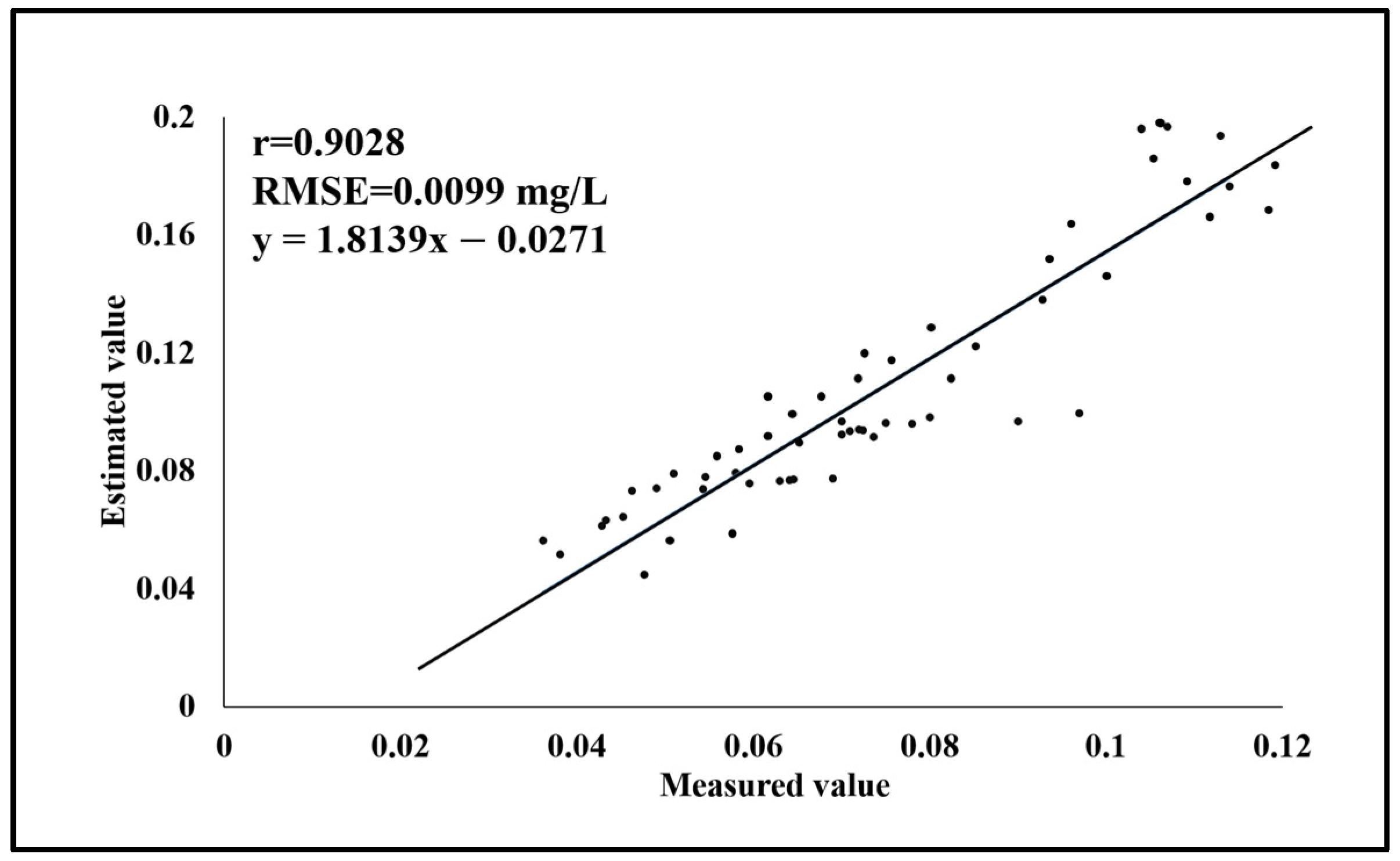
2. Materials and Methods

2.1. Study Area

The Changshan Islands are the largest island group in the Yellow Sea, and they are located between 38°55′ to 39°41′ north and 122°04′ to 123°32′ east, covering an area of 10,324 km2. The Changshan Islands have the typical characteristics of an archipelago ecosystem. Figure 1 shows the location of the study area. The northwest of the Changshan Islands is connected to the Liaodong Peninsula, and the whole area is rich in marine resources. In recent years, with the development of large-scale economic activities such as tourism, transportation, industry, and aquaculture, land-based and island-derived pollutants have entered the archipelago area. The main pollution sources for DIN in the area are marine aquaculture [18], industrial discharge [39,40], port seawater pollution [41], tourist garbage [42], and river discharge [43]. In order to study the influence of each driving factor on marine water quality and refine the spatial and temporal distribution of the water quality changes, it was necessary to analyze the sensitivity of the ocean water quality conditions and influencing factors over a wide range, with a long time series and high precision.

2.2. Experimental Data

2.2.1. Measured Data

In this study, the NH4-N, NO2-N, and NO3-N contents were investigated in the whole coastal area of Changshan Islands from 2013 to 2022. The data sampling was carried out using continuous measurement, i.e., the data were sampled twice at the same point in the spring tide and neap tide each month, and 25 samples of NH4-N, NO2-N, and NO3-N were collected at one-hour sampling intervals in each sampling task. The data were analyzed in the laboratory, and the average value of 50 samples for the two tides at the same point was taken as the measured value of the month at that point. The DIN detection instruments and analysis methods for the measured data are listed in Table 1. There were 320 measured sets of data for each DIN over the 10 years, and the data were randomly and evenly distributed within the waters of the Changshan Islands, for which the maximum value of NH4-N was 0.318 mg/L, and the minimum value was 0.006 mg/L. The maximum value of NO3-N was 0.164 mg/L, and the minimum value was 0 mg/L. The maximum value of NO2-N was 0.015 mg/L, and the minimum value was 0 mg/L.

2.2.2. Remote Sensing Data

The remote sensing data were Landsat 8 multi-spectral remote sensing images with a spatial resolution of 30 m, which can meet the needs of mesoscale water quality inversion. Compared with large-scale water quality monitoring, this approach can improve the spatial location matching accuracy with the measured data and also allows the use of more accurate location coordinates in the model calculation. The remote sensing satellite data were obtained from the United States Geological Survey EarthExplorer website (https://earthexplorer.usgs.gov/, accessed on 1 May 2022). We selected the images with the most similar survey time to the measured data, and the row numbers included (119, 32) and (119, 33). The Operational Land Imager (OLI) sensor has a total of nine bands, and Band 1–Band 7 were selected in this study, which are the coastal zone, blue, green, red, near-infrared, short-wavelength infrared 1, and short-wavelength infrared 2 bands, respectively. The band range was 0.433 µm to 2.300 µm. The panchromatic Band 8 for enhanced resolution and the cirrus Band 9 for cloud detection were not used in this study. In addition, all the above data are Landsat 8 Collection 2 Level-2 (L2) products, which do not require radiometric calibration or atmospheric correction.

2.3. Experimental Procedure

As shown in Figure 2 the experiments of this study were divided into three parts: data preprocessing, model training, and plotting the distribution of the three nitrogen compounds.
  • Step 1: data preprocessing. The image with the closest measured data collection time was selected (image revisiting period is 16 days), and the remote sensing reflectance of its closest image raster position was selected based on the spatial location coordinates of the three nitrogen samples (spatial resolution is 30 m). The bands with a high correlation with NH4-N, NO2-N, and NO3-N were judged using Pearson correlation coefficients and used as the characteristic bands. The measured values, spatial characteristics (longitude and latitude), and characteristic bands of the three inorganic nitrogen forms/species were composed into a sample dataset. The sample dataset was then processed by removing outliers by IBM SPSS Statistics 22 and performing dequantization, which only scales the data characteristics and eliminates the influence of correlation between data due to the difference of the quantization, but it also keeps the coefficient of variation and the degree of mutual influence between parameters unchanged [44,45].
  • Step 2: model training. The sample datasets of all three nitrogen compounds were divided into training and test sets in the ratio of 8:2 [19], with the characteristic bands and spatial features as the input parameters and the actual measured values of the inorganic nitrogen forms/species as the target parameters. The regression results for NH4-N, NO2-N, and NO3-N were obtained by training the S-WSVR model, where the characteristic bands were used to calculate the weights in the multivariate weighting module. The regression results were evaluated using five accuracy indicators, and the training results for the three nitrogen compounds at the same point were summed and compared with the actual DIN values to verify the model accuracy.
  • Step 3: mapping the distribution of the three nitrogen compounds. The image data from the spring and autumn of 2013–2022 were selected, and the images with the same time and rank numbers (119, 32) and (119, 33) were stitched and cropped. The characteristic bands and spatial feature information of the processed images were read and input into the trained regression model to calculate the concentrations of the three nitrogen compounds, and the calculated results were divided into 10 classes to plot the spatial and temporal distributions of NH4-N, NO2-N, and NO3-N.

2.4. Model Method

2.4.1. Support Vector Regression

Previous studies have shown that SVR models perform well in the case of limited samples [17,46]. SVR is used to control the number of margins and support vectors using kernel functions, sparse solutions, and Vapnik–Chervonenkis core theory [47,48]. A linear regression hyperplane is then found in the high-dimensional feature space to solve the nonlinear supervised learning. In this study, the input parameter space information, the selected feature bands, and the target parameters of NH4-N, NO2-N, and NO3-N were considered to have a nonlinear relationship. Assuming a certain inorganic nitrogen forms/species training sample as N = x 1 , n 1 , ( x 2 , n 2 ) , , ( x m , n m ) , n m R , the SVR model was constructed as follows:
f x = ω T x + b
where ω is a normal vector, which determines the characteristic hyperplane direction; b is the displacement constant; x is the input relevant parameter; n is the inorganic nitrogen forms/species measured value; m is the inorganic nitrogen forms/species sample size; and f x is the inorganic nitrogen forms/species estimate.
The goal of SVR is to minimize the “distance” to the inorganic nitrogen forms/species sample points farthest from the hyperplane. Unlike other regressions, SVR can be conducted with the deviation ε between f x and n to seek a maximum “interval band”, so that more sample points are located in the interval band. Losses are computed only for sample points outside the interval band, where the absolute value of the deviation of f x from n is greater than ε. Relaxation variables are introduced to cope with nonlinearities and outliers, and points are allowed to exist outside the interval band, so that the losses should be as small as possible. The soft interval SVR model can be denoted as follows:
m i n ω , b   1 2 ω 2 + C i = 1 m ( ξ i , ξ i ) s . t .   f x n m ε + ξ i n m f x ε + ξ i ξ i ,   ξ i 0 ,   i = 1,2 , , m
where C is the regularization constant that provides a balance between the smoothness of the fitting function and the bias of the training data; ξ i , ξ i * is a positive relaxation variable; ε represents the allowable fit tolerance; and m indicates the actual number of data.
At the same time, by introducing Lagrange multipliers, the original space of the input data is mapped to a higher-dimensional feature space, and the optimal feature hyperplane is obtained by a nonlinear kernel function. The inorganic nitrogen forms/species inversion model SVR, after introducing the Lagrange multipliers, can be denoted as follows:
  f x = i = 1 m α i α i κ x , x i + b
where α i * , α I is a Lagrange multiplier greater than or equal to 0, and κ x , x i is the kernel function.
The kernel function learning method extends linear learning to nonlinear learning by “kernelization”, for which the commonly used functions include a linear kernel, polynomial kernel, s-type kernel, and radial basis function (RBF) kernel. The RBF kernel was selected as the kernel function for the quantitative inversion of seawater nitrogen compounds in this study, and its formula is as follows:
κ x , x i = exp { x x i 2 σ 2   }
where σ is the Gaussian kernel bandwidth.

2.4.2. Multivariate Weighting Module

Each characteristic band contains different amounts of information about the target inorganic nitrogen forms/species, so there is variability in the contribution of the characteristic bands to the target parameters in the fitting calculation process. The traditional algorithms represented by single bands and band combinations tend to lose important information in the inversion, so we added a multivariate weighting module to the basic model. The weighting can assign higher weights to the bands with less intra-class variation and more inter-class variation, to retain more effective information and improve the fitting accuracy. The multivariate weighting module is based on the statistical idea of using the Mahalanobis distance metric to find the central distance between samples to determine the inter-sample similarity. Compared with other similarity measures, the Mahalanobis distance calculation is based on the overall samples and can take into account the correlation between individual samples. It is also independent of the measurement scale [49,50,51], so when discriminating between the three nitrogen compounds and their characteristic bands, the Mahalanobis distance can solve the problem of similarity between samples. Therefore, the Mahalanobis distance can resolve the non-independent homogeneous distribution between the characteristic bands without considering the different measurement units of the three nitrogen compounds and the band reflectance when determining the similarity between the nitrogen compounds and their characteristic bands. In this study, we finally chose to calculate the similarity between the three nitrogen compounds and their associated bands using the Mahalanobis distance to set the weights. The formula for the Mahalanobis distance in calculating the weights between the inorganic nitrogen forms/species and the associated bands is as follows:
M D ( q i , N ) = q i N T 1 ( q i N ) i = 1,2 , , n
where I represents the selected bands with a high correlation with inorganic nitrogen forms/species; N is the actual measurement value of the sample of collected inorganic nitrogen forms/species; n is the number of characteristic bands with inorganic nitrogen forms/species; and is the estimated parameters and all the associated band covariance matrices, which is a measure of the correlation between variables in a multidimensional dataset, as shown in Equation (6):
= v a r ( N )   c o v ( q 1 , N )   v a r ( q 1 )   c o v ( q 2 , N )   c o v ( q 2 , q 1 )   v a r ( q 2 )   .   .   .   .   .   .   .   .   .   .   .   .   c o v ( q n , N )   c o v ( q n , q 1 )   c o v ( q n , q 2 )   . . .   v a r ( q n )
where v a r is the variance and c o v is the covariance.

2.4.3. S-WSVR

The multiple weighted regression model that takes into account spatial features (S-WSVR) is a model that builds a regression relationship based on the SVR model with spatial features (longitude and latitude) and feature bands as the model input parameters. It incorporates a multivariate weighting module to calculate the weighting coefficients for the feature bands and uses the nitrogen and salt concentrations as the output parameters. The algorithm inputs spatial features into the model and makes the feature bands have unequal weight calculations in the regression fitting process, thereby retaining more useful information and improving the model fitting capability. Figure 3 shows the model structure of S-WSVR, which can be represented as follows:
N = f s p a c e , w l a n d s a t = f L O N , L A T ,   W B A N D
where L O N , L A T stand for the geographical latitude and longitude, respectively. W B A N D represents the product of the feature band and the Mahalanobis distance weight.

3. Results

3.1. Characteristic Bands and Weights

The proposed approach is based on the use of the Pearson correlation coefficient in the multivariate statistical method to determine the correlation between the Landsat 8 band reflectance and the three nitrogen compounds, and the whole process is realized in SPSS statistical software. The Pearson correlation coefficient is widely used to measure the correlation degree between two variables, where the value indicates the correlation between the two variables. In order to avoid the loss of information and to ensure the correct selection of correlated bands, the Pearson correlation coefficient was used as the judgment indicator when selecting the correlated bands. The Landsat 8 bands with high correlation with NH4-N, NO2-N, and NO3-N are, respectively, B2, B3, B4, B5, B6, and B7; B3, B6, and B7; and B5, B6, and B7. These bands were taken as the characteristic bands. Table 2 lists the Pearson correlation coefficients and the significance for NH4-N, NO2-N, NO3-N, and the band reflectance.
The S-WSVR model calculation was implemented based on PyCharm Community Edition 2021.3.3. The longitude, latitude, and characteristic bands of the training set of the three nitrogen compounds were input into the algorithm, and the weighting coefficients of the characteristic bands of the three nitrogen compounds were obtained using the multivariate weighting module. This allows the relevant bands to have unequal weight calculations in the subsequent fitting regression. The weighting coefficients calculated by Equation (5) of the feature bands of the three nitrogen compounds are listed in Table 3.

3.2. Regression Results

The weighting coefficients calculated by the multivariate weighting module were multiplied by the values of the characteristic bands, and the spatial features were trained with the three inorganic nitrogen forms/species concentration values of the training set as the learning target. A genetic algorithm was used for the optimization process to avoid overfitting during the training process. The three inorganic nitrogen forms/species concentration of the test set was finally output and the regression fitting results were evaluated for accuracy using the Pearson correlation coefficient (r), root-mean-square error (RMSE), mean square error (MSE), mean absolute error (MAE), and mean absolute percentage error (MAPE) for the regression training results and the measured values. The formulas for the model evaluation equations are as follows:
r = 1 i = 1 n ( N i ^ N i ) 2 i = 1 n ( N i ¯ N i ) 2
R M S E = 1 n i = 1 n ( N i ^ N i ) 2
M S E = 1 n i = 1 n ( N i ^ N i ) 2
M A E = 1 n i = 1 n N i ^ N i
M A P E = 1 n i = 1 n N i ^ N i N i
where N i ^ is the predicted value for the three inorganic nitrogen forms/species, N i is the measured value for the three inorganic nitrogen forms/species, N i ¯ is the average value of the measured three inorganic nitrogen forms/species, and n is the number of test sets.
The regression results for the NH4-N, NO2-N, and NO3-N model training are shown in Figure 4a–c, respectively, with r-values of 0.9063, 0.8900, and 0.9755, and RMSE values of 0.2097 mg/L, 0.1230 mg/L, and 0.1573 mg/L, respectively. In addition, we used the same training and test sets to compare the integrated ordinary linear regression (OLR), the geographically weighted regression (GWR), the original model (SVR), the fused spatio-temporal model (S-SVR), the multiple weighted regression model (WSVR), and the fused spatio-temporal multiple weighted regression model (S-WSVR). From Table 4, it can be found that OLR models have the worst performance results, and the WSVR and S-WSVR models with the addition of the multivariate weighting module show a certain magnitude of improvement over both the SVR and S-SVR fitting results (r), with a minimum improvement of 0.0222 and a maximum improvement of 0.2160, indicating that the multivariate weighting module can effectively filter out more effective information in the feature bands and make the relevant bands improve the accuracy in the fitting process. In addition, GWR, S-SVR, and S-WSVR training results are better, indicating that the regression relationship between water quality value and the band reflectance value of the selected bands is significantly nonstationary in space. Table 5 shows that there is a strong correlation between longitude and latitude and the three nitrogen compounds, and after adding spatial features to the input parameters, S-SVR and S-WSVR show a substantial improvement in fitting accuracy over SVR and WSVR, with a minimum improvement of 0.3833 and a maximum improvement of 0.4659, which shows that the addition of spatial features can improve the fitting accuracy. The S-WSVR model takes into account the spatial information, and the band-weighted comparison of the other three models shows that the S-WSVR model shows the best performance and the highest fitting accuracy. The fitting accuracy r-values are increased by 0.4353, 0.4535, and 0.5210, compared with the original SVR model, and the RMSE, MSE, MAE, and MAPE values are reduced. The experiments prove that the S-WSVR model can obtain good fitting results for all three nitrogen compounds in this mesoscale archipelagic sea area.
To further validate the model performance, the DIN concentration, i.e., the sum of the NH4-N, NO2-N, and NO3-N measured values, was calculated based on the measured data and compared with the measured DIN values. Figure 5 and Table 6 show the DIN fitting accuracy evaluation indices. The sum of the predicted values of the three nitrogen compounds, compared with the actual DIN, has a fitting accuracy r-value of 0.9028 and an RMSE of 0.0990 mg/L, and the accuracy evaluation of DIN compared with the three nitrogen compounds has a ranking of r-value of NO3-N > NH4-N > DIN > NO2-N and an error accuracy ranking of NH4-N > NO2-N > NO3-N > DIN. The accuracy ranking shows that the fitting accuracy r-value of DIN is not as high as that of NO3-N and NH4-N, but the RMSE accuracy ranking is the smallest, which indicates that the S-WSVR model has no overfitting phenomenon for the prediction of the three nitrogen compounds. The sum of the predicted results of the three nitrogen compounds correlates well with the DIN, so that the DIN content can be judged by the predicted results of the S-WSVR model.

4. Discussion

4.1. Representation of the Weights in the Model

The goal of the SVR model is to find the optimal hyperplane in high-dimensional space with the smallest “distance” of the farthest sample points. The sample points falling into the “spacing band” under an equal weight calculation will lose some correct information. In order to allow more correlated band features to be selected in the “interval band”, more useful information can be obtained in the SVR model calculation, and the sample points can be stretched to be closer to the optimal hyperplane by assigning weight coefficients to the correlated bands [52,53]. In addition, from the comparison between Table 2 and Table 3, it can be found that, the larger the r-value, the smaller the weight is, and vice versa. To explain this phenomenon, we selected some NO3-N(z), B5(x), and B6(y) data for regression, and assigned a larger weight to B5(y) for the regression to compare the role of band weighting in the regression model. Figure 6 shows the data point distance from the hyperplane location, where the data point in Figure 6b is close to the hyperplane. The essence of this is that the weighting is a stretching change to the B6 data to make B5 more favorable to the model convergence, to reduce the losses.
Figure 7 shows the projection of the points in the hyperplane on the B5-o-NO3-N plane and the B6-o-NO3-N plane, respectively. After weighting B6, the r-value of the B5-o-NO3-N plane increases and the RMSE decreases. The correlation of B5 with NH4-N increases and the r-value of the B6-o-NO3-N plane decreases and the RMSE increases. The correlation of B6 with NH4-N decreases, which is due to the large weight given to B6. In summary, when using the distance weighting idea in the SVR prediction model, weighting the bands with a small degree of correlation can improve the prediction accuracy of the model [54].

4.2. Spatio-Temporal Distribution of the Three Nitrogen Compounds

Since the sea surface can be ice-covered in the winter and the air is cloudy in the summer in the study area, we selected high-quality images from the spring and autumn, and after data preprocessing, the images were input into the regression models for the three inorganic nitrogen forms/species after training. The variation trends are similar to the results obtained by Li et al. [55] and Yang et al. [56]. The spatial and temporal distribution of NH4-N, NO2-N, and NO3-N in the spring and autumn from 2013 to 2022 are shown in Figure 8. We referred to Camargo et al. [13] to classify the distribution results into 10 classes of inorganic nitrogen forms/species toxicity. The first nine classes for NH4-N and NO2-N are low toxicity, but the 10th class is more toxic [32]. NO3-N has no toxicity but was also divided into 10 classes according to the minimum to maximum value. In 2013–2022, the average value of NH4-N in the spring was 0.040 mg/L and in the autumn, it was 0.045 mg/L. The average concentration of NO2-N was 0.003 mg/L in the spring and 0.004 mg/L in the autumn. The average concentration of NO3-N was 0.062 mg/L in the spring and 0.069 mg/L in the autumn. The average concentrations of the three nitrogen compounds are higher in the autumn than in the spring, which is mainly due to the influence of biological activities. Plankton growth is active in the spring and weakens in the autumn. As a result, the nitrogen consumption is high in the spring, so that the seawater has a higher content of the three nitrogen compounds in the autumn than in the spring.
The lowest value of NH4-N content was 0 mg/L in both the spring and autumn of 2013. The lowest value was no longer 0 mg/L after the spring of 2014, indicating that the whole sea area was polluted by NH4-N after 2014. From 2014, the Changhai county government vigorously developed island tourism and mariculture activities. The NH4-N concentration in the whole sea area in the spring and autumn has increased since 2014, but marine organisms in the aquaculture area need to absorb a lot of nitrogen to grow in the spring, so the area with a higher NH4-N concentration in spring has become less. NO2-N is an intermediate product of the nitrification reaction of NH4-N under conditions of sufficient oxygen, and NO3-N can also undergo denitrification to produce NO2-N in an anaerobic environment [38]. NO2-N reached a maximum of 0.015 mg/L in the spring of 2019, while the minimum value of 0 mg/L occurred each year. The formation of NO3-N has a lag, and human activities increased after 2014. In 2013–2014, human activities in the offshore waters of Liaodong Peninsula were weak, and the NO3-N in the spring had a period of low concentration. On the other hand, the DIN discharged from the Yalu River is five times higher than that of other rivers flowing into the North Yellow Sea waters [56], and NO3-N is the main form present. The volume of river water flowing into the sea in the spring is larger than that in the autumn due to the influence of rainfall, so the concentration on the east side of the study area is generally higher in the spring than in the autumn. In summary, the whole study area from 2013 to 2022 was enhanced by human activities after 2014 and subject to increased NH4-N pollution, but the NO2-N content was relatively stable and the NO3-N content was no greater than 0.18 mg/L, indicating that the seawater still maintained a stable state for self-cleaning and the seawater environment was in a relatively balanced state.
In addition to the characteristics of the temporal changes, the spatial distribution of the three nitrogen compounds shows a certain pattern. The southwestern part of the study area receives the influence of human activities on the one hand and the water exchange near the Bohai Strait on the other, making the NH4-N content higher than in the other areas. The central part features a marine reserve and a large volume of algae farming activities, making the NH4-N content in this area the least abundant. The northeastern part of the area is affected by the discharge of the Yalu River, and the NH4-N content increases slightly. The central part is close to the wide sea area away from the source of pollution, but with the changes in the flow of the ocean, it is also slightly polluted by NH4-N. NO2-N shows the characteristic of a gradually decreasing concentration from the northeast to the southwest, mainly because the organic matter in the Yalu River is particularly high and the oxygen consumption of suspended bacteria and organisms is also very high, and the lower the dissolved oxygen content, the higher the NO2-N concentration [14,35]. The NO3-N content decreases in the southwest of the study area with the residential islands as the center, and the NO3-N concentration increases in the east and northeast under the influence of the Yalu River discharge. The concentration decreases in the central offshore area with fewer human activities, while the concentration is lower in the central distant sea area away from frequent human activities.
In the NO3-N spatial and temporal variation maps for spring 2014, autumn 2014, autumn 2015, and autumn 2017, the study area on the east side shows a higher concentration of NO3-N. NO3-N is the end product of inorganic nitrogen purification, and NO3-N accumulates in the ocean until nitrogen-fixing organisms solidify NO3-N to further purify the water. The accumulated NO3-N concentration changes with the movement of the current. Figure 9 shows the superimposed flow field and NO3-N concentration in the spring of 2014 and 2019 in the eastern area. When the flow velocity decreases, the NO3-N flow will be weakened, and the NO3-N concentration will temporarily increase. Meanwhile, the NO3-N will disperse as the flow velocity increases and the flow direction changes, but this transient concentration increase still does not cause harm to the marine environment.

4.3. Influencing Factors for the Three Nitrogen Compounds

From the previous section, it can be inferred that human activities are the main influencing factors for NH4-N and NO3-N, while the DO content is the main influencing factor for NO2-N, so in this section, we analyze these two important influencing factors in depth. In order to better elaborate the influence of human activities on the three nitrogen compounds, Figure 10 divides the whole study area into four zones:
  • A is the southwest zone of the study area, which has a dense population and is close to the inshore area in the south of Liaodong Peninsula.
  • B is the offshore area in the middle of the study area, where there are several marine reserves and reservation areas and large areas of shellfish and algae farming.
  • C is the northeast zone of the study area, which is also one of the areas closest to the discharge of the Yalu River.
  • D is the area near the open sea.

4.3.1. Impact of Sea Area Use on NH4-N and NO3-N

As shown in Figure 10, there are 49 sea area functional zones (AFZs) in the study area, including reserved areas, port and shipping areas, industrial and urban sea use areas, marine protected areas, mineral and energy areas, tourism and recreation areas, agriculture and fishery areas, and special use areas. The SQRHM model can quantitatively analyze the degree of impact of human activities on marine ecosystems with the following equations:
I = i = 1 m F i × D i d i D i
I c = j = 1 s I j × W j
where I   is the impact of a human activity on each spatial location, m is the number of spatial locations of human activity, i is the action point (the action point is the center of the human activity area), F i is the intensity of the first action point of the human activity, D i is the maximum impact distance of the first action point of the human activity, d i is the distance between the unit point and action point i of the human activity, I c denotes the combined impact of multiple human activities on the cell site, s denotes the presence of type s human activities, j denotes the j th human activity, I j is the impact of the j th human activity on the cell site, and W j is the weight of the j th human activity in the comprehensive evaluation [57].
Seven evaluation indicators were selected for the evaluation of the degree of impact of human activities on the marine ecosystem in the Changshan Islands sea area: reclaimed land area, aquaculture raft area, tourism development area, port navigation area, mineral resources area, marine protected area, and reserved area. The reclaimed land area is the cumulative reclaimed land area from 2013 to 2022, and the total reclaimed area is less than 10 km2. The aquaculture raft area, as shown in Figure 11, is the area of aquaculture rafts in 2022. The other data were calculated according to the planned area, and we referred to the results of the study of Li et al. [57] to assign the role intensity and weight in Table 7. The final results were classified into four levels from weak to strong, as shown in Table 8. The final degrees of human activity impact in 2022 in areas A–D were, respectively, very strong impact, strong impact, and medium impact.
Although both areas A and B are strongly affected by human activities, the results of the nitrogen concentration in areas A and B are different. The main impact of area B is the floating raft aquaculture in the surface layer. The large number of shellfish and seagrasses cultured in the surface layer of seawater can absorb NH4-N for growth. Secondly, there are many marine protected areas and reserved areas in area B with better environmental protection of seawater quality, and although land reclamation has been carried out in area B, the influence of the area is relatively small and low, so NH4-N pollution in Area B is low. On the other hand, area A has been greatly impacted by tourism development and pollution from harbor shipping, so the NH4-N pollution is more serious. In addition, NO3-N concentration is highest in the northeast of area A and the southwest of area B, i.e., centered on the residential islands, which are the areas where human activities have the strongest impact on the ecosystem. These areas are also the most sensitive areas for seawater pollution. Area C is strongly affected by human activities, and the NH4-N and NO3-N concentrations show a certain increase. Area D is less affected by human activities, and NH4-N and NO3-N pollution decrease with distance from human activities. In summary, human activities have a strong influence on NH4-N and NO3-N, and the more frequent the human activities, the stronger the pollution.

4.3.2. Dissolved Oxygen Environment

The Yalu River, with an annual runoff of 32.76 billion m3, is the largest seaward river in the entire North Yellow Sea, and studies have shown that hypoxia often occurs at the mouth of the river due to its high oxygen consumption [58]. However, this phenomenon usually occurs at the bottom of the water body, while the DO content in the surface layer is more adequate, compared with the bottom layer. To prove that the spatial and temporal distribution of NO2-N concentration corresponds to the DO content, the average of the measured DO data in the surface layer of the seawater in areas A, B, and C in the spring and autumn of 2018–2020 was recorded.
As shown in Figure 12, the DO content in the surface seawater is ranked as A > B > C, which is the result of the unique geographical characteristics of the study area. Area A is closer to the wide sea than area C, where the wind is greater and the waves are bigger. As a result, the DO content in area A is higher than that in area C. The surface water quality is more serious and is closer to the mouth of the Yalu River, and the NO2-N concentration is A < B < C. Meanwhile, the DO content in the spring is higher than that in the autumn, showing obvious seasonal characteristics. The spring flood of the Yalu River caused greater river flow in the spring than that in the autumn of the same year. Thus, the greater river flow in the spring leads to a higher DO content; on the contrary, the DO content in the autumn is lower. In summary, the DO content of the surface water of the Changshan Islands and the distance to the mouth of the Yalu River are positively correlated, while the NO2-N concentration is negatively correlated with the DO content. Therefore, to control the NO2-N concentration within a certain range, the discharge of the Yalu River needs to be regulated.

5. Conclusions

In this paper, a multiple weighted regression (S-WSVR) model taking into account spatial information has been proposed to monitor the continuous distribution of NH4-N, NO2-N, and NO3-N in the surface layer of the seawater in a mesoscale archipelagic environment, which smooths the spatial complexity of the mesoscale water quality distribution and retains more useful information in the characteristic bands. Based on the Mahalanobis distance and mathematical and statistical analysis, the contribution of the different characteristic wavebands was calculated, and the spatial information was utilized as one of the input parameters. The accuracy of the experimental results for NH4-N, NO2-N, and NO3-N was better than that of the original model, with r-values of 0.9063, 0.8900, and 0.9755 and RMSEs of 0.2097 mg/L, 0.1230 mg/L, and 0.1573 mg/L, respectively, which represent an increase in r-value of 43.53%, 45.35%, and 52.10% and a decrease in RMSE of 0.0487 mg/L, 0.2977 mg/L, and 0.1571 mg/L, respectively, compared with the original model. The accuracy was improved the most by the spatial information, while the multivariate weighting resulted in a small improvement, which proves that the three nitrogen compounds are nonlinear and heterogeneous in spatial distribution, and the contributions of the characteristic bands in the calculation are different. Moreover, the inversion results for the three nitrogen compounds were summed and compared to the measured DIN concentration, obtaining an r-value of 0.9028. In addition, we also obtained the characteristic bands associated with Landsat 8 for the three nitrogen compounds: B2, B3, B4, B5, B6, and B7 for NH4-N; B3, B6, and B7 for NO2-N; and B5, B6, and B7 for NO3-N.
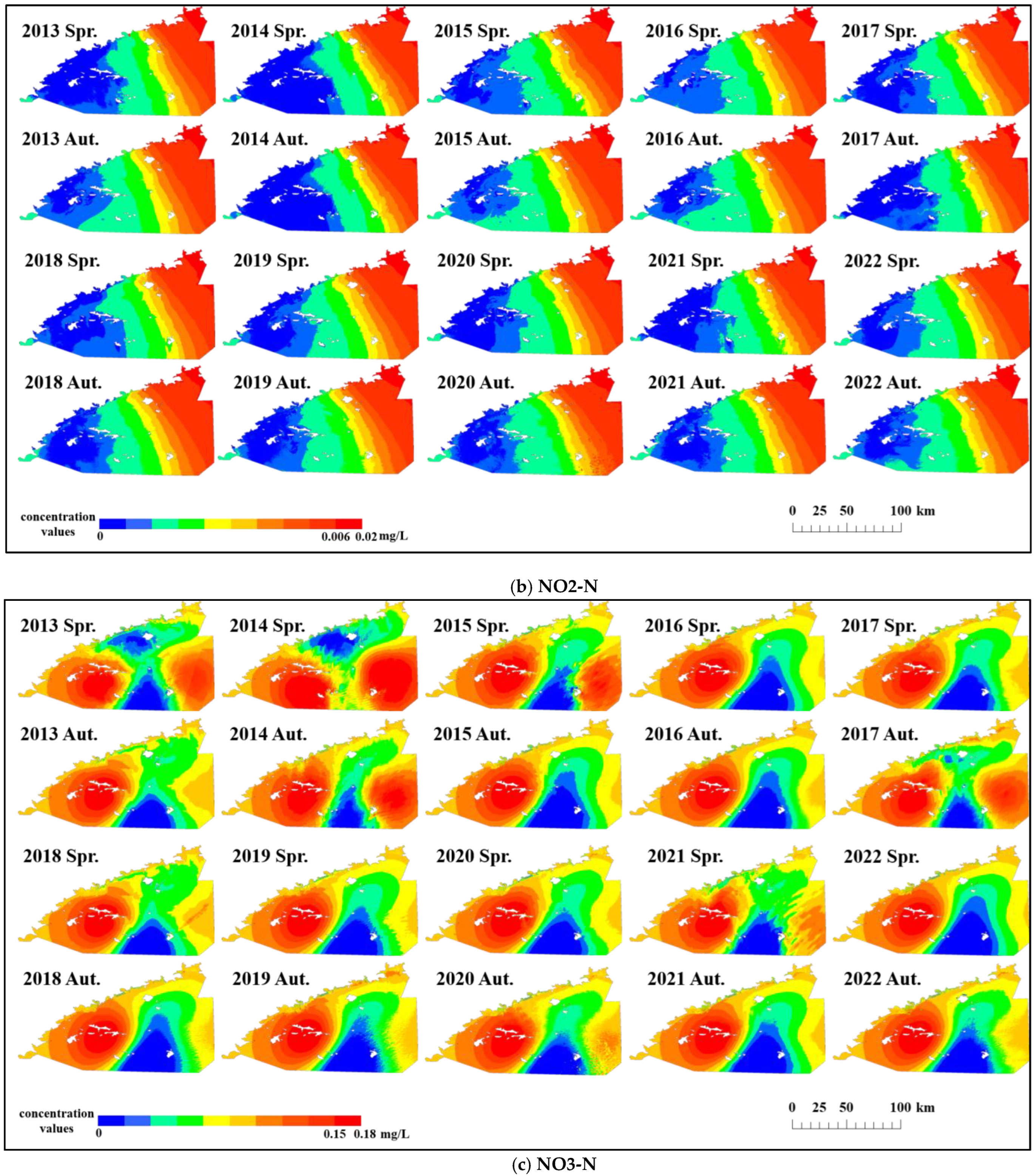
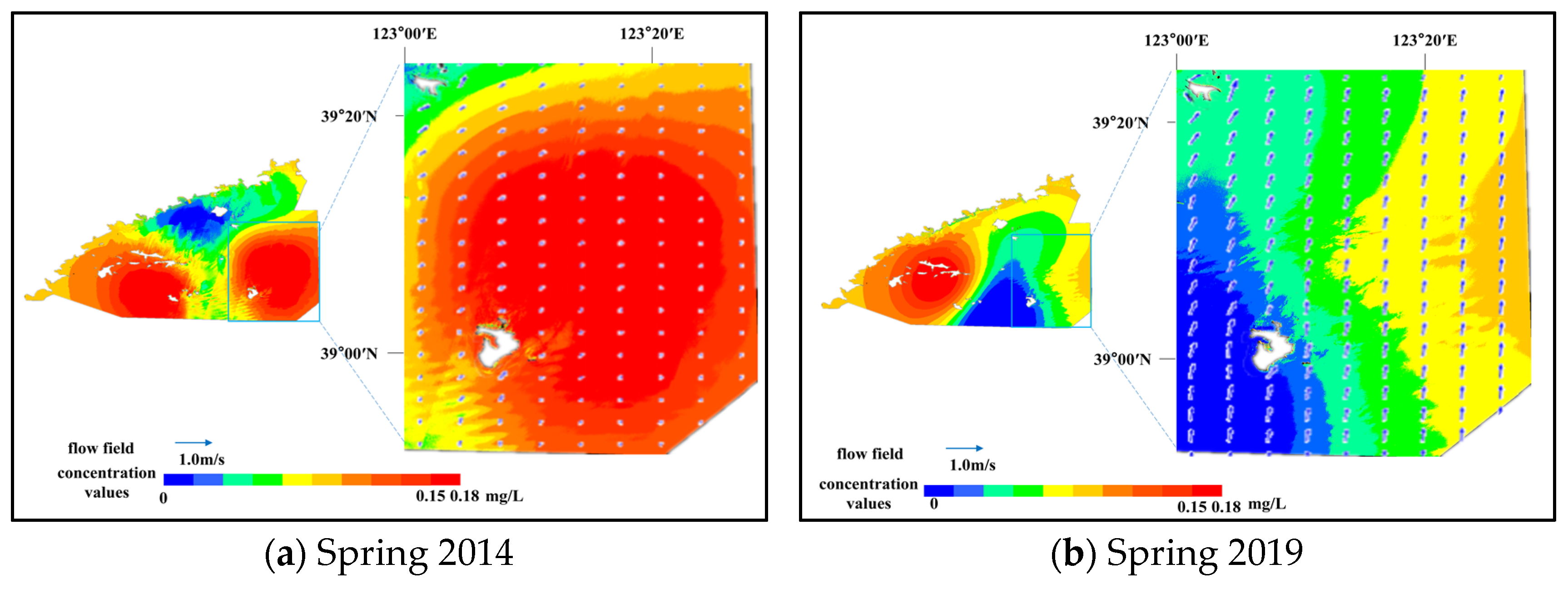
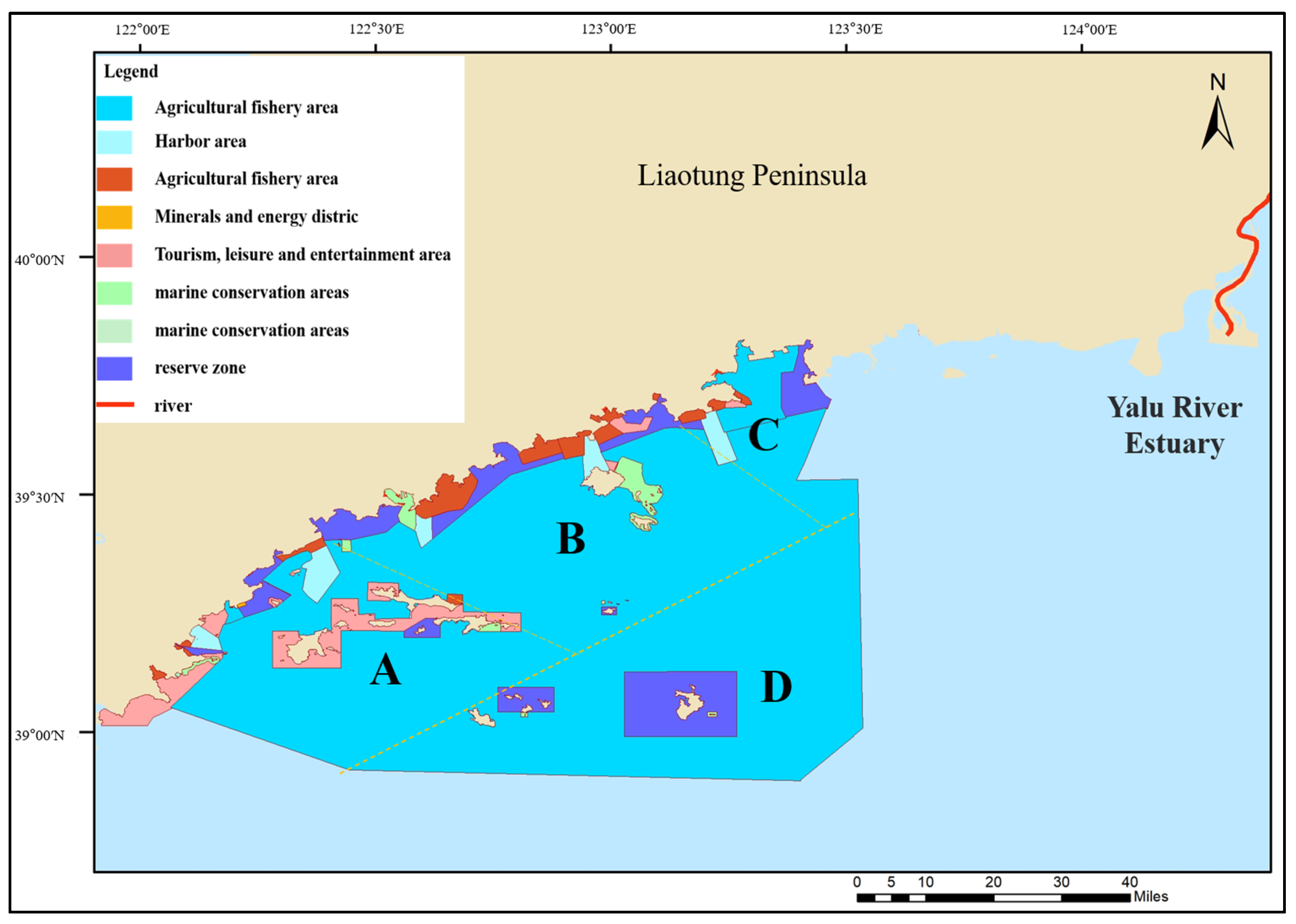
Furthermore, we input the 2013–2022 images into the S-WSVR model to plot the spatial and temporal distributions of NH4-N, NO2-N, and NO3-N. The distribution patterns of the three nitrogen compounds in the Changshan Islands area were then analyzed from the spatio-temporal distribution map. It was found that the Changshan Islands sea area has been polluted by DIN in the whole area since 2014, but the seawater is still in a relatively healthy state. The SQRHM analysis revealed that the intensity of human activities had a greater impact on NH4-N and NO3-N. Human daily life on the islands, tourism development, and harbor shipping were the main sources of pollution, and shellfish and algae on surface culture floating rafts were conducive to nitrogen purification. In addition, the water body discharged by the Yalu River is anoxic, and the closer the sea area is to the estuary of the Yalu River, the lower the DO content and the higher the NO2-N content. Overall, the pollution concentration of inorganic nitrogen decreases with the distance from human activities, and it is necessary to regulate human activities and the Yalu River discharge in order to protect the ecological environment of this sea area.
Consequently, this study shows that the S-WSVR model can monitor the three inorganic nitrogen forms/species content in seawater comprehensively at the island archipelago scale and then thoroughly monitor the seawater DIN condition, which can thus be used to monitor the seawater environment. However, the similarity between the relevant bands of the model and the inorganic nitrogen forms/species will be changed by the external conditions of the measured data. Therefore, the degree of the contribution of the relevant bands to the different inorganic nitrogen forms/species will also be changed by the external conditions of the measured data, so the weight coefficients need to be adjusted when using the modified model, which requires more quasi-real-time measured data. In the future, the input parameters could be adjusted to improve the correlation with inorganic nitrogen forms/species by combining the bands and then calculating the similarity with inorganic nitrogen forms/species, so that more valid information can be retained to further improve the accuracy.

Author Contributions

Conceptualization, X.L. and J.Q.; methodology, X.L., J.Q., H.Z. and B.Z.; software, X.L. and H.Z.; validation, X.L., Y.Y. and G.X.; writing—original draft preparation, X.L.; writing—review and editing, J.Q., W.S., B.Z. and J.D.; visualization, X.L., H.Z. and Y.Y.; project administration, X.L., J.Q. and W.S.; funding acquisition, W.S., B.Z. and J.D.; investigation, X.L., Y.Y. and G.X. All authors have read and agreed to the published version of the manuscript.

Funding

This work was supported in part by the National Natural Science Foundation of China under grant numbers 42071343 and 42071428 and 42204031.

Institutional Review Board Statement

Not applicable.

Informed Consent Statement

Not applicable.

Data Availability Statement

The data used in this study are available upon request.

Acknowledgments

We would like to thank the Dalian Huangbohai Marine Surveying Data Information Co., Ltd.(Dalian, China) for providing the inorganic nitrogen data and dissolved oxygen data for the Changshan Islands area for scientific research. We would like to thank the National Marine Environmental Monitoring Center for providing the Functional zoning of the sea area and flow field data for the Changshan Islands area for scientific research.

Conflicts of Interest

The authors declare no conflict of interest.

References

  1. Keitt, B.; Campbell, K.; Saunders, A.; Clout, M.N.; Tershy, B. The Global Islands Invasive Vertebrate Eradication Database: A Tool to Improve and Facilitate Restoration of Island Ecosystems; Island Invasives: Eradication and Management; IUCN: Gland, Switzerland, 2011; pp. 74–77. [Google Scholar]
  2. Chi, Y.; Zhang, Z.; Xie, Z.; Wang, J. How human activities influence the island ecosystem through damaging the natural ecosystem and supporting the social ecosystem? J. Clean. Prod. 2020, 248, 119203. [Google Scholar] [CrossRef]
  3. Cao, W.; Zhou, Y.; Li, R.; Li, X.; Zhang, H. Monitoring long-term annual urban expansion (1986–2017) in the largest archipelago of China. Sci. Total Environ. 2021, 776, 146015. [Google Scholar] [CrossRef]
  4. Zhang, J.; Wang, D.R.; Jennerjahn, T.; Dsikowitzky, L. Land–sea interactions at the east coast of Hainan Island, South China Sea: A synthesis. Cont. Shelf Res. 2013, 57, 132–142. [Google Scholar] [CrossRef]
  5. Royle, S.A. Geography of Islands; Routledge: London, UK, 2002. [Google Scholar]
  6. Zhang, P.; Ruan, H.; Dai, P.; Zhao, L.; Zhang, J. Spatiotemporal river flux and composition of nutrients affecting adjacent coastal water quality in Hainan Island, China. J. Hydrol. 2020, 591, 125293. [Google Scholar] [CrossRef]
  7. Ilter Turkdogan Aydinol, F.; Kanat, G.; Bayhan, H. Sea water quality assessment of Prince Islands’ Beaches in Istanbul. Environ. Monit. Assess. 2012, 184, 149–160. [Google Scholar] [CrossRef] [PubMed]
  8. Kim, K.T.; Kim, E.S. Seawater Quality of Jinhae Bay and Adjacent Sea of Gaduk Island, Korea. In Proceedings of the KOSOMES Biannual Meeting; The Korean Society of Marine Environment and Safety: Ansan, Republic of Korea, 2009; pp. 137–143. [Google Scholar]
  9. Jha, D.K.; Vinithkumar, N.V.; Sahu, B.K.; Dheenan, P.S.; Das, A.K.; Begum, M.; Devi, M.P.; Kirubagaran, R. Multivariate and geo-spatial approach for seawater quality of Chidiyatappu Bay, south Andaman Islands, India. Mar. Pollut. Bull. 2015, 96, 463–470. [Google Scholar] [CrossRef] [PubMed]
  10. Gavio, B.; Palmer-Cantillo, S.; Mancera, J.E. Historical analysis (2000–2005) of the coastal water quality in San Andrés Island, SeaFlower Biosphere Reserve, Caribbean Colombia. Mar. Pollut. Bull. 2010, 60, 1018–1030. [Google Scholar] [CrossRef]
  11. Wannicke, N.; Frey, C.; Law, C.S.; Voss, M. The response of the marine nitrogen cycle to ocean acidification. Glob. Chang. Biol. 2018, 24, 5031–5043. [Google Scholar] [CrossRef]
  12. Sellner, K.G.; Doucette, G.J.; Kirkpatrick, G.J. Harmful algal blooms: Causes, impacts and detection. J. Ind. Microbiol. Biotechnol. 2003, 30, 383–406. [Google Scholar] [CrossRef]
  13. Camargo, J.A.; Alonso, Á. Ecological and toxicological effects of inorganic nitrogen pollution in aquatic ecosystems: A global assessment. Environ. Int. 2006, 32, 831–849. [Google Scholar] [CrossRef]
  14. Breitburg, D.; Levin, L.A.; Oschlies, A.; Gregoire, M.; Chavez, F.P.; Conley, D.J.; Garcon, V.; Gilbert, D.; Gutierrez, D.; Isensee, K.; et al. Declining oxygen in the global ocean and coastal waters. Science 2018, 359, eaam7240. [Google Scholar] [CrossRef] [PubMed]
  15. Gao, J.; Yao, F.; Lei, X.; Wang, J.; Mang, F. Study on water quality evaluation and water quality distribution characteristics of main stream of Daduhe River under background of cascade hydropower development. Water Resour. Hydropower Eng. 2021, 52, 133–145. [Google Scholar]
  16. Bierman, P.; Lewis, M.; Ostendorf, B.; Tanner, J. A review of methods for analysing spatial and temporal patterns in coastal water quality. Ecol. Indic. 2011, 11, 103–114. [Google Scholar] [CrossRef]
  17. Guo, H.; Huang, J.J.; Chen, B.; Guo, X.; Singh, V.P. A machine learning-based strategy for estimating non-optically active water quality parameters using Sentinel-2 imagery. Int. J. Remote Sens. 2021, 42, 1841–1866. [Google Scholar] [CrossRef]
  18. Li, X.; Liu, B.; Zheng, G.; Ren, Y.; Zhang, S.; Liu, Y.; Gao, L.; Liu, Y.; Zhang, B.; Wang, F. Deep-learning-based information mining from ocean remote-sensing imagery. Natl. Sci. Rev. 2020, 7, 1584–1605. [Google Scholar] [CrossRef] [PubMed]
  19. Huang, J.; Wang, D.; Gong, F.; Bai, Y.; He, X. Changes in Nutrient Concentrations in Shenzhen Bay Detected Using Landsat Imagery between 1988 and 2020. Remote Sens. 2021, 13, 3469. [Google Scholar] [CrossRef]
  20. Vieitez, M.O.; Ivanov, T.I.; Ubachs, W.; Lewis, B.R.; de Lange, C.A. On the complexity of the absorption spectrum of molecular nitrogen. J. Mol. Liq. 2008, 141, 110–117. [Google Scholar] [CrossRef]
  21. Isenstein, E.M.; Park, M.H. Assessment of nutrient distributions in Lake Champlain using satellite remote sensing. J. Environ. Sci. 2014, 26, 1831–1836. [Google Scholar] [CrossRef]
  22. Li, Y.; Zhang, Y.; Shi, K.; Zhu, G.; Zhuo, Y.; Zhang, Y.; Guo, Y. Monitoring spatiotemporal variations in nutrients in a large drinking water reservoir and their relationships with hydrological and meteorological conditions based on Landsat 8 imagery. Sci. Total Environ. 2017, 599–600, 1705–1717. [Google Scholar] [CrossRef]
  23. Yu, X.; Yi, H.; Liu, X.; Wang, Y.; Liu, X.; Zhang, H. Remote-sensing estimation of dissolved inorganic nitrogen concentration in the Bohai Sea using band combinations derived from MODIS data. Int. J. Remote Sens. 2016, 37, 327–340. [Google Scholar] [CrossRef]
  24. Wang, X.; Fu, L.; He, C. Applying support vector regression to water quality modelling by remote sensing data. Int. J. Remote Sens. 2011, 32, 8615–8627. [Google Scholar] [CrossRef]
  25. Vakili, T.; Amanollahi, J. Determination of optically inactive water quality variables using Landsat 8 data: A case study in Geshlagh reservoir affected by agricultural land use. J. Clean. Prod. 2020, 247, 119134. [Google Scholar] [CrossRef]
  26. Li, X.; Zheng, H.; Liu, Y.; Wan, W. Multi-source data machine learning-based study on method for regional water quality prediction. Water Resour. Hydropower Eng. 2021, 52, 152–163. [Google Scholar]
  27. Du, Z.; Qi, J.; Wu, S.; Zhang, F.; Liu, R. A spatially weighted neural network based water quality assessment method for large-scale coastal areas. Environ. Sci. Technol. 2021, 55, 2553–2563. [Google Scholar] [CrossRef] [PubMed]
  28. Du, Z.; Wu, S.; Zhang, F.; Liu, R.; Zhou, Y. Extending geographically and temporally weighted regression to account for both spatiotemporal heterogeneity and seasonal variations in coastal seas. Ecol. Inform. 2018, 43, 185–199. [Google Scholar] [CrossRef]
  29. Dimitrakopoulos, P.G.; Koukoulas, S.; Michelaki, C.; Galanidis, A. Anthropogenic and environmental determinants of alien plant species spatial distribution on an island scale. Sci. Total Environ. 2022, 805, 150314. [Google Scholar] [CrossRef] [PubMed]
  30. Wang, H.; Tian, T.; Gong, Y.; Ma, S.; Altaf, M.M.; Wu, H.; Diao, X. Both environmental and spatial variables affect bacterial functional diversity in mangrove sediments at an island scale. Sci. Total Environ. 2020, 753, 142054. [Google Scholar] [CrossRef] [PubMed]
  31. Torbick, N.; Hession, S.; Hagen, S.; Wiangwang, N.; Becker, B.; Qi, J. Mapping inland lake water quality across the Lower Peninsula of Michigan using Landsat TM imagery. Int. J. Remote Sens. 2013, 34, 7607–7624. [Google Scholar] [CrossRef]
  32. Constable, M.; Charlton, M.; Jensen, F.; McDonald, K.; Craig, G.; Taylor, K.W. An Ecological Risk Assessment of Ammonia in the Aquatic Environment. Hum. Ecol. Risk Assess. 2003, 9, 527–548. [Google Scholar] [CrossRef]
  33. Thurston, R.V.; Russo, R.C.; Vinogradov, G.A. Ammonia toxicity to fishes. Effect of pH on the toxicity of the unionized ammonia species. Environ. Sci. Technol. 1981, 15, 837–840. [Google Scholar] [CrossRef]
  34. Lin, K.; Zhu, Y.; Zhang, Y.; Lin, H. Determination of ammonia nitrogen in natural waters: Recent advances and applications. Trends Environ. Anal. Chem. 2019, 24, e00073. [Google Scholar] [CrossRef]
  35. Jensen, F.B. Nitrite disrupts multiple physiological functions in aquatic animals. Comp. Biochem. Physiol. Part A Mol. Integr. Physiol. 2003, 135, 9–24. [Google Scholar] [CrossRef] [PubMed]
  36. Kir, M.; Sunar, M.C. Acute Toxicity of Ammonia and Nitrite to Sea Bream, Sparus aurata (Linnaeus, 1758), in Relation to Salinity. J. World Aquac. Soc. 2018, 49, 516–522. [Google Scholar] [CrossRef]
  37. Nichols, C.P. Temporal and Spatial Variability of Metal Distributions in Staten Island Marsh-Creek Systems: Does Connectivity to the Arthur Kill Impact Anthropogenic Enrichment, Sediment Quality and Toxicity Potential in NY/NJ He Marsh Habitats? City University of New York: New York, NY, USA, 2012. [Google Scholar]
  38. Zehr, J.P.; Kudela, R.M. Nitrogen cycle of the open ocean: From genes to ecosystems. Annu. Rev. Mar. Sci. 2011, 3, 197–225. [Google Scholar] [CrossRef] [PubMed]
  39. Wahyuningsih, S.; Effendi, H.; Wardiatno, Y. Nitrogen removal of aquaculture wastewater in aquaponic recirculation system. Aquac. Aquar. Conserv. Legis. 2015, 8, 491–499. [Google Scholar]
  40. Zhu, G.; Peng, Y.; Li, B.; Gou, J.; Wang, S. Biological removal of nitrogen from wastewater. In Reviews of Environmental Contamination and Toxicology; Springer: New York, NY, USA, 2008; pp. 159–195. [Google Scholar]
  41. Gupta, A.K.; Gupta, S.K.; Patil, R.S. Statistical analyses of coastal water quality for a port and harbour region in India. Environ. Monit. Assess. 2005, 102, 179–200. [Google Scholar] [CrossRef] [PubMed]
  42. Mukherjee, A.; Chakraborty, S.; Das, S.; De, T.K. Dynamics of dissolved inorganic nitrogen in bioturbated littoral surface sediments at a selected tourist destination of Northern Coastal Bay of Bengal, India: An ecologically significant case study. Braz. J. Biol. Sci. 2018, 5, 799–814. [Google Scholar] [CrossRef]
  43. Green, P.A.; Vörösmarty, C.J.; Meybeck, M.; Galloway, J.N.; Peterson, B.J.; Boyer, E.W. Pre-industrial and contemporary fluxes of nitrogen through rivers: A global assessment based on typology. Biogeochemistry 2004, 68, 71–105. [Google Scholar] [CrossRef]
  44. Zheng, A.; Casari, A. Feature Engineering for Machine Learning: Principles and Techniques for Data Scientists; O’Reilly Media, Inc.: Sebastopol, CA, USA, 2018. [Google Scholar]
  45. Caruana, R.; Niculescu-Mizil, A. An empirical comparison of supervised learning algorithms. In Proceedings of the 23rd International Conference on Machine Learning, Ithaca, NY, USA, 25–29 June 2006; pp. 161–168. [Google Scholar]
  46. Chen, L.; Ren, C.; Zhang, B.; Wang, Z.; Xi, Y. Estimation of forest above-ground biomass by geographically weighted regression and machine learning with sentinel imagery. Forests 2018, 9, 582. [Google Scholar] [CrossRef]
  47. Smola, A.J.; Schölkopf, B. A tutorial on support vector regression. Stat. Comput. 2004, 14, 199–222. [Google Scholar] [CrossRef]
  48. Awad, M.; Khanna, R. Support vector regression. In Efficient Learning Machines; Apress: Berkeley, CA, USA, 2015; pp. 67–80. [Google Scholar]
  49. Loghmari, M.A.; Naceur, M.S.; Boussema, M.R. A Spectral and Spatial Source Separation of Multispectral Images. IEEE Trans. Geosci. Remote Sens. 2006, 44, 3659–3673. [Google Scholar] [CrossRef]
  50. Jarvis, R.A.; Patrick, E.A. Clustering using a similarity measure based on shared near neighbors. IEEE Trans. Comput. 1973, 100, 1025–1034. [Google Scholar] [CrossRef]
  51. Chang, C.I.; Ji, B. Weighted abundance-constrained linear spectral mixture analysis. IEEE Trans. Geosci. Remote Sens. 2006, 44, 378–388. [Google Scholar] [CrossRef]
  52. Han, X.; Clemmensen, L. On Weighted Support Vector Regression. Qual. Reliab. Eng. Int. 2015, 30, 891–903. [Google Scholar] [CrossRef]
  53. Xu, Y.; Wang, L. A weighted twin support vector regression. Knowl. Based Syst. 2012, 33, 92–101. [Google Scholar] [CrossRef]
  54. Zhu, H.; Zhang, B.; Song, W.; Dai, J.; Lan, X.; Chang, X. Power-Weighted Prediction of Photovoltaic Power Generation in the Context of Structural Equation Modeling. Sustainability 2023, 15, 10808. [Google Scholar] [CrossRef]
  55. Li, Y.W.; Hu, Y.Y.; Chen, S.M. Distribution and influence factors of nutrients in the North Yellow Sea in Summer and Autumn. Zhongguo Huanjing Kexue/China Environ. Sci. 2013, 33, 1060–1067. [Google Scholar]
  56. Yang, J.; Zhang, G.L.; Zheng, L.X.; Zhang, F. Seasonal variations of fluxes and distributions of dissolved N2O in the North Yellow Sea. Huan Jing Ke Xue 2009, 30, 656–662. [Google Scholar]
  57. Li, Y.; Song, X.; Wu, Z. An integrated methodology for quantitative assessment on impact of human activities on marine ecosystems: A case study in Laizhou Bay, China. Oceanol. Limnol. Sin. 2015, 46, 133–139. [Google Scholar]
  58. Zhu, Z.-Y.; Zhang, J.; Wu, Y.; Zhang, Y.-Y.; Lin, J.; Liu, S.-M. Hypoxia off the Changjiang (Yangtze River) Estuary: Oxygen depletion and organic matter decomposition. Mar. Chem. 2011, 125, 108–116. [Google Scholar] [CrossRef]
Figure 1. Study area location map diagram for the Changshan Islands.
Water 15 03176 g001
Figure 2. Experimental flowchart.
Water 15 03176 g002
Figure 3. The multiple weighted regression model, considering spatial characteristics, orange arrows represent longitude, and green arrows represent latitude.
Water 15 03176 g003
Figure 4. The regression results for NH4-N, NO2-N, and NO3-N.
Water 15 03176 g004
Figure 5. The regression results for the measured DIN values and the estimated values of the sum of the three nitrogen compounds.
Water 15 03176 g005
Figure 6. Correlated band weighting before and after comparison. (a) B6 schematic diagram of unweighted convergence. (b) B6 weighted convergence.
Water 15 03176 g006
Figure 7. Higher feature band weighting anterior-posterior projection comparison.
Water 15 03176 g007
Figure 8. Ten-year distribution results for NH4-N, NO2-N, and NO3-N in the sea area of Changshan Islands from 2013 to 2022.
Water 15 03176 g008aWater 15 03176 g008b
Figure 9. The relationship between the NO3-N concentration change and the flow field on the east side of the study area.
Water 15 03176 g009
Figure 10. Functional zoning of the sea area in the study area and the location of the Yalu River mouth.
Water 15 03176 g010
Figure 11. Visual interpretation of the aquaculture raft area.
Water 15 03176 g011
Figure 12. Histograms of dissolved oxygen and nitrite nitrogen levels in areas A, B, and C of the study area, 2018–2020.
Water 15 03176 g012
Table 1. DIN data analysis methods and instruments.
Nitrogen CompoundAnalytical MethodInstrument
NH4-NSubbromate oxidation processHINOTEK 752N UV-VIS spectrophotometer
NO2-NZinc-cadmium reduction processHINOTEK 752N UV-VIS spectrophotometer
NO3-NN-(1-Naphthyl) ethylenediamine
spectrophotometry
HINOTEK 752N UV-VIS spectrophotometer
DINion\
Table 2. The Pearson correlation coefficients and the significance for NH4-N, NO2-N, NO3-N, and the band reflectance.
Nitrogen CompoundBand r p
NH4-NB1−0.176 *<0.05
B2−0.228 **<0.01
B30.374 **<0.01
B4−0.330 **<0.01
B5−0.323 **<0.01
B6−0.237 **<0.01
B7−0.207 **<0.01
NO2-NB10.013>0.05
B2−0.028>0.05
B3−0.262 **<0.01
B4−0.106>0.05
B5−0.168 *<0.05
B6−0.322 **<0.01
B7−0.313 **<0.01
NO3-NB1−0.01>0.05
B2−0.041>0.05
B30.008>0.05
B40.052>0.05
B50.344 **<0.01
B6−0.203 **<0.01
B7−0.245 **<0.01
Notes: * correlation is significant at the 0.05; ** correlation is significant at the 0.01.
Table 3. The weighting coefficients of the characteristic bands of NH4-N, NO2-N, and NO3-N.
Nitrogen CompoundBandWeight
NH4-NB21.5502
B31.5256
B41.5382
B51.5409
B61.5439
B71.5506
NO2-NB31.7298
B61.6949
B71.7041
NO3-NB51.4045
B61.4444
B71.4413
Table 4. The regression results for the SVR, S-SVR, WSVR, and S-WSVR models.
rRMSEMSEMAEMAPE
NH4-NOLR0.18190.53760.28910.39720.5152
GWR0.63620.33300.07120.22840.3704
SVR0.47100.28870.08330.23790.3806
WSVR0.60280.25300.06400.20040.3522
S-SVR0.87700.24500.06000.16530.3455
S-WSVR0.90630.20970.04400.12540.2972
NO2-NOLR0.11150.56550.31970.45410.5275
GWR0.51310.26450.06590.19210.2899
SVR0.36900.28010.07840.20400.3012
WSVR0.58500.24400.05950.18090.2709
S-SVR0.83490.17660.03120.11370.2729
S-WSVR0.89000.15730.02470.10030.2638
NO3-NOLR0.17920.76820.59020.59961.0117
GWR0.68350.39860.18970.39010.6279
SVR0.52200.45600.20790.42410.6896
WSVR0.54500.45570.20770.41070.6664
S-SVR0.95330.23660.05600.12550.2960
S-WSVR0.97550.12800.02830.04570.1872
Table 5. The Pearson correlation coefficients and significance of NH4-N, NO2-N, and NO3-N and latitude and longitude.
Spatial InformationNH4-NNO2-NNO3-N
r p r p r p
Longitude0.403 **<0.010.272 **<0.010.400 **<0.01
Latitude0.272 **<0.010.355 **<0.010.262 **<0.01
Note: ** correlation is significant at the 0.01.
Table 6. The error table for the sum of the three nitrogen compounds and the DIN fitting regression results.
MSEMAEMAPE
DIN0.00090.03050.1523
Table 7. The Pearson correlation coefficients and the significance of NH4-N, NO2-N, NO3-N, and latitude and longitude.
Evaluation IndicatorStrength of ActionWeighting Value
00.250.50.751
Reclaimed land area (km2)-<1010–3030–50≥500.246
Surface aquaculture raft area (km2)--<1010–100≥1000.131
Tourism development area (km2)-<1010–2020–30≥300.074
Area of port shipping (km2)--<1010–100≥1000.074
Mineral resources area (km2)--<2020–100≥1000.245
Grade of Marine Protected Area-Prefectural and MunicipalProvincialCountryWorld0.120
Grade of reserved area-Prefectural and MunicipalProvincialCountryWorld0.120
Table 8. Degree of influence of human activities on the marine ecosystem.
I c Degree of Influence
0–0.25Slight influence
0.25–0.5Moderate influence
0.5–0.75Strong influence
0.75–1Very strong influence
Disclaimer/Publisher’s Note: The statements, opinions and data contained in all publications are solely those of the individual author(s) and contributor(s) and not of MDPI and/or the editor(s). MDPI and/or the editor(s) disclaim responsibility for any injury to people or property resulting from any ideas, methods, instructions or products referred to in the content.

