Article

A Simplified Method for Effective Calculation of 3D Slope Reliability

1
School of Civil Engineering, Hefei University of Technology, Hefei 230009, China
2
School of Civil Engineering and Architecture, Ningbo Tech University, Ningbo 315100, China
*
Author to whom correspondence should be addressed.
Water 2023, 15(17), 3139; https://doi.org/10.3390/w15173139
Submission received: 18 July 2023 / Revised: 25 August 2023 / Accepted: 29 August 2023 / Published: 1 September 2023
(This article belongs to the Special Issue Risk Management Technologies for Deep Excavations in Water-Rich Areas)

Abstract

:
Traditional 3D slope reliability analysis methods have high computational costs and are difficult to popularize in engineering practice. Under the framework of the limit equilibrium method with 3D slip surface normal stress correction, the critical horizontal acceleration coefficient K c , which is equivalent to the safety factor F s , is selected to characterize the slope stability. The limit state function uses the difference between K c and the known critical value K c 0 . A simplified method for calculating the reliability of 3D slope is proposed. Through two typical slope examples, the 3D reliability calculation results of six methods after coupling two limit state functions and three reliability algorithms are compared. The results show that this method is reliable and effective, and the method coupled with subset simulation (SS) is the one with good calculation accuracy and efficiency. In the case of long slopes, 2D analysis results may underestimate the probability of slope instability, and 3D reliability of the slope must be analyzed.

1. Introduction

Slope stability evaluation is one of the important and popular research topics in geotechnical engineering. Due to the existence of complex loads and geological conditions, as well as the inherent variability of soil physical and mechanical parameters, slope failure is actually uncertain [1]. The influence of these uncertain factors on slope stability cannot be considered by a single safety factor [2]. Slope reliability analysis is a useful supplement to the deterministic method of slope stability [3].
In the past few decades, the research on slope reliability analysis methods has developed rapidly and achieved many meaningful results. However, most researchers simplified the slope stability analysis problems into two-dimensional plane strain problems, ignoring the three-dimensional effects of actual slopes, which will overestimate or underestimate their stabilities [4,5,6]. Especially for slopes with obvious longitudinal changes in soil properties along the slope surface, concentrated loads acting on the surface, irregular potential failure surfaces, or short slopes with non-negligible boundary conditions, their 3D effects are particularly significant, and 3D reliability analysis must be carried out [7].
Three-dimensional slope reliability analysis requires higher computational costs than two-dimensional simulation, and sometimes the calculation time is even more than one month [8]. This is one of the reasons why 3D slope reliability analysis cannot be widely used in practical engineering. However, in the preliminary design of highway engineering, it is often necessary to quickly evaluate the stability of slopes of hundreds of sections [9]. In the study of 3D slope reinforcement measures, it is also necessary to quickly judge the effects of different reinforcement measures [10,11]. In these cases, there is an urgent need for a method that can quickly perform 3D slope reliability analysis without significant loss of accuracy.
In recent years, the research on 3D slope reliability analysis methods has gradually increased with the improvement of computer performance. The existing 3D slope reliability analysis methods mainly include the analytical method [12,13], stochastic finite element method (SFEM) [1,14], stochastic limit equilibrium method (SLEM) [15], and stochastic limit analysis method (SLAM) [16]. The research of these methods is carried out under the framework of combining the deterministic method of 3D slope stability and the reliability calculation method. The limit state performance function generally adopts the expression form of the difference between safety factor F s and one. The obvious differences in accuracy and computational efficiency of various methods are mainly derived from the efficiency of the solution method of safety factor and the reliability algorithm. The analytical method has a small amount of calculation, but it is difficult to apply in engineering practice because the sliding surface must be a special combination shape with a cylindrical surface in the middle and a vertical plane or an ellipsoid surface at both ends. Based on the finite element method and strength reduction technology, the stochastic finite element method has the advantage of automatically obtaining the critical sliding surface. However, when the probability of slope failure is very small, its computational cost is very high [17]. The stochastic limit analysis method constructs the static allowable stress field or the maneuvering allowable velocity field according to the large-scale geotechnical parameter samples, based on the lower bound theorem or the upper bound theorem. The safety factor of the slope is solved by means of mathematical programming. If the number of soil parameter samples is large, the calculation efficiency is low. Therefore, the stochastic limit equilibrium method with a clear concept and high computational efficiency is still the most widely used method in engineering practice.
The conventional 3D slope limit equilibrium methods are obtained by extending the 2D slice methods. According to the different assumptions of the inter-column force, they can be divided into the 3D simplified Bishop method [18,19], 3D simplified Janbu method [18,19], 3D Morgenstern–Price method [20,21], and so on. Safety factor expressions are usually complex nonlinear implicit expressions, which require multiple numerical iterations to solve, and sometimes encounter non-convergence problems. Some scholars used the stochastic response surface method (SRSM) [22], intelligent response surface method (IRSM) [23], genetic algorithm (GA) [8], support vector machine (SVM) [4], and other surrogate models to simplify complex nonlinear implicit performance functions into approximate equivalent explicit expressions, which effectively solves the difficult problem of 3D slope reliability calculation. However, these methods require a large amount of data to generate enough samples to obtain surrogate models. For highly nonlinear and small failure probability problems, it is difficult to fit the surrogate models.
Sarma [24] proposed a good idea to replace the safety factor with a critical horizontal acceleration coefficient K c for slope stability analysis. In the process of solving K c , no numerical iteration occurs, and no non-convergence problem will be encountered. However, the formula of the Sarma method is cumbersome and the solving process is not very convenient. Zhu [25] proposed an explicit solution for the 3D slope safety factor by correcting the normal stresses on the slip surface. His method does not need to assume the inter-column force, so it does not belong to the “column method”. The calculation principle of the method is simple without iteration and non-convergence problems, and the calculation results are reliable. In this paper, a new method for calculating the reliability of the 3D slope was proposed by using the critical horizontal acceleration coefficient as the criterion of slope stability under the mode of the 3D limit equilibrium method with normal stress correction of the sliding surface.
Among the reliability algorithms, the Monte Carlo simulation (MCS) method is the most widely used because of its simple concept. As long as there are enough samples, the approximate accurate reliability calculation results can be obtained. However, in the case of slopes with small failure probability, the calculation is very time-consuming. The subset simulation method (SS) reduces the sample requirements and is an efficient method for solving the reliability analysis of slopes with small failure probability [26]. In this paper, the subset simulation method is used to calculate the reliability of the 3D slope.
In the author’s previous work [27], it has been proved that the limit state performance function using the critical horizontal acceleration coefficient expression can indeed significantly improve the computational efficiency probability of 2D slope reliability. In this paper, we extend the previous work to the 3D slope and comprehensively study the accuracy and efficiency of the obtained algorithm.
The research framework of this paper is as follows. Firstly, based on the 3D limit equilibrium method with normal stress correction on the sliding surface, four main equilibrium equations including the critical horizontal acceleration coefficient and three correction parameters were established. Secondly, according to the definition of the critical horizontal acceleration coefficient, its explicit expression was derived. Thirdly, a simplified method for calculating the reliability of the three-dimensional slope is proposed by using the difference expression between the critical horizontal acceleration coefficient and the critical value and combining it with the reliability algorithm. Finally, the effectiveness and reliability of the proposed method are verified by two slope examples.

2. Three-Dimensional Limit Equilibrium Method Based on the Modification of Normal Stresses over Slip Surface

2.1. Fundamental Assumptions

A 3D slope with a general shape sliding surface and a coordinate system are shown in Figure 1a. It is assumed that the horizontal projections of the sliding direction of each point on the sliding surface are parallel to each other and opposite to the positive direction of the x-axis. The slope surface is represented by g x , y , and the sliding surface is represented by s x , y . The slope is divided into many soil columns. As shown in Figure 1b, one of the soil columns has a width of d x and a length of d y . The horizontal projection area of the soil column is d A , and the angles with the x and y axes are α x and α y , respectively. The angle between the outer normal direction and the z-axis is γ z .
According to the geometric relation, d A can be calculated by Equation (1).
d A = Δ d x d y
where
Δ = 1 + s x 2 + s y 2
s x = tan α x ,   s y = tan α y
cos γ z = 1 1 + s x 2 + s y 2 = 1 Δ
Assuming that the soil column weight is w x , y and the horizontal acceleration coefficient is K , then the horizontal seismic force is K w x , y , and the position of the action point is x , y , z c .
There are normal stress and shear stress at the bottom of the column, which are expressed by σ x , y and τ x , y , respectively. The pore water pressure is expressed by u x , y . The cohesion and effective internal friction angle of the soil at the sliding surface are c x , y and ϕ x , y , respectively.
The direction cosines of the normal force and shear force at the bottom of the column are n σ x , n σ y , n σ z and n τ x , n τ y , n τ z , respectively. As the sliding direction is parallel to the x -axis, n τ y = 0 . From the geometrical relation, it follows that
n σ x , n σ y , n σ z = s x Δ , s y Δ , 1 Δ
n τ x , n τ y , n τ z = 1 Δ , 0 , s x Δ
where
Δ = 1 + s x 2
In order to simplify the calculation, the initial normal stress distribution σ 0 ( x , y ) on the sliding surface adopts the 3D extended form of the Fellenius method [28].
σ 0 ( x , y ) = w ( x , y ) 1 + s x 2 + s y 2
The initial normal stresses over the slip surface need to be corrected to make the 3D sliding body meet the required equilibrium conditions. Let the correction function be ξ x , y , then
σ x , y = σ 0 ( x , y ) ξ x , y

2.2. Three-Dimensional Limit Equilibrium Equations

For 3D slopes, only the reliability calculation results that rigorously meet the force balance in three directions and the moment balance conditions around three axes are accurate. The research shows that the quasi-rigorous solution is very close to the rigorous solution, and the difference can be ignored. The former is more suitable for practical engineering [25]. Therefore, in order to solve the problem of rapid analysis of 3D slope reliability, a quasi-rigorous simplified method of 3D slope reliability based on four main equilibrium equations of the sliding body is proposed.
When the 3D sliding body reaches the limit equilibrium state under the action of the force in three directions and the torque around the y-axis, the following equations can be listed (in order to simplify, “ x , y ” in all formulas are omitted.):
σ n σ y d A = 0
σ n σ x + τ n τ x   d A = K w d x d y
σ n σ z + τ n τ z   d A = w d x d y
σ n σ z + τ n τ z x d A σ n σ x + τ n τ x s d A = w x d x d y K w z c d x d y
Substituting Equations (7) and (8) into Equation (10a–d) leads to
σ s y d x d y = 0
σ s x + τ Δ Δ d x d y = K w d x d y
σ + s x Δ Δ τ d x d y = w d x d y
σ + s x Δ Δ τ x d x d y σ s x + τ Δ Δ s d x d y = w x d x d y K w z c d x d y
It is assumed that safety factor values of the entire sliding surface are equal, and the relationship between normal stress and shear stress obeys the Mohr–Coulomb failure criterion.
τ = 1 F s σ u tan φ + c
Let
ψ = tan φ
c u = c u tan φ
ρ = Δ Δ
Equation (11a–d) is rearranged as
σ s y d x d y = 0
s x + ρ ψ F s σ d x d y = K w d x d y 1 F s ρ c u d x d y
1 + ρ ψ s x F s σ d x d y = w d x d y 1 F s s x ρ c u d x d y
x + s s x + ρ ψ x s x s F s σ d x d y = w x d x d y K w z c d x d y 1 F s ρ x s x s c u d x d y
In order to make Equation (14a–d) statically determinate and solvable, the correction function must contain three undetermined parameters and its general form can be taken as
ξ ( x , y ) = ξ 0 + λ 1 ξ 1 + λ 2 ξ 2 + λ 3 ξ 3
Substituting Equations (12) and (15) into Equation (14a–d), we can obtain
λ 1 D 1 + λ 2 D 2 + λ 3 D 3 = E
λ 1 A 11 + B 11 F s + λ 2 A 12 + B 12 F s + λ 3 A 13 + B 13 F s + K G 1 = A 14 + B 14 F s
λ 1 A 21 + B 21 F s + λ 2 A 22 + B 22 F s + λ 3 A 23 + B 23 F s + K G 2 = A 24 + B 24 F s
λ 1 A 31 + B 31 F s + λ 2 A 32 + B 32 F s + λ 3 A 33 + B 33 F s + K G 3 = A 34 + B 34 F s
where
D i = σ 0 ξ i s y d x d y i = 1 , 2 , 3 E = σ 0 ξ 0 s y d x d y
A 1 i = σ 0 ξ i s x d x d y ( i = 1 , 2 , 3 ) A 14 = σ 0 ξ 0 s x d x d y
A 2 i = σ 0 ξ i d x d y ( i = 1 , 2 , 3 ) A 24 = w d x d y σ 0 ξ 0 d x d y
A 3 i = σ 0 ξ i x + s s x d x d y ( i = 1 , 2 , 3 ) A 34 = [ w x σ 0 ξ 0 x + s s x ]   d x d y
B 1 i = ρ ψ σ 0 ξ i d x d y ( i = 1 , 2 , 3 ) B 14 = ρ c u + ψ σ 0 ξ 0   d x d y
B 2 i = ρ ψ σ 0 ξ i s x d x d y ( i = 1 , 2 , 3 ) B 24 = ρ c u + ψ σ 0 ξ 0 s x d x d y
B 3 i = ρ ψ σ 0 ξ i x s x s d x d y ( i = 1 , 2 , 3 ) B 34 = ρ x s x s c u + ψ σ 0 ξ 0   d x d y
G 1 = w d x d y G 2 = 0
G 3 = w z c d x d y
Assuming that safety factor F s is a known parameter and the initial normal stress distribution σ 0 is determined, then D 1 ~ D 3 , A 11 ~ A 14 , A 21 ~ A 24 , A 31 ~ A 34 , B 11 ~ B 14 , B 21 ~ B 24 , B 31 ~ B 34 , G 1 ~ G 3 , and E , these parameters can be solved by a definite integral. Substituting the 31 parameters into Equation (16a–d), we can obtain the statically determinate solvable limit equilibrium equations with four unknowns λ 1 , λ 2 , λ 3 and K .
Equation (16a–d) can be rewritten in a matrix form
D 1 D 2 D 3 0 A 11 + B 11 F s A 12 + B 12 F s A 13 + B 13 F s G 1 A 21 + B 21 F s A 22 + B 22 F s A 23 + B 23 F s G 2 A 31 + B 31 F s A 32 + B 32 F s A 33 + B 33 F s G 3 λ 1 λ 2 λ 3 K = E A 14 + B 14 F s A 24 + B 24 F s A 34 + B 34 F s
According to Cramer’s rule, λ 1 , λ 2 , λ 3 and K can be solved.
λ 1 = Δ 1 Δ 0
λ 2 = Δ 2 Δ 0
λ 3 = Δ 3 Δ 0
K = Δ 4 Δ 0
where
Δ 0 = D 1 D 2 D 3 0 A 11 + B 11 F s A 12 + B 12 F s A 13 + B 13 F s G 1 A 21 + B 21 F s A 22 + B 22 F s A 23 + B 23 F s G 2 A 31 + B 31 F s A 32 + B 32 F s A 33 + B 33 F s G 3
Δ 1 = E D 2 D 3 0 A 14 + B 14 F s A 12 + B 12 F s A 13 + B 13 F s G 1 A 24 + B 24 F s A 22 + B 22 F s A 23 + B 23 F s G 2 A 34 + B 34 F s A 32 + B 32 F s A 33 + B 33 F s G 3
Δ 2 = D 1 E D 3 0 A 11 + B 11 F s A 14 + B 14 F s A 13 + B 13 F s G 1 A 21 + B 21 F s A 24 + B 24 F s A 23 + B 23 F s G 2 A 31 + B 31 F s A 34 + B 34 F s A 33 + B 33 F s G 3
Δ 3 = D 1 D 2 E 0 A 11 + B 11 F s A 12 + B 12 F s A 14 + B 14 F s G 1 A 21 + B 21 F s A 22 + B 22 F s A 24 + B 24 F s G 2 A 31 + B 31 F s A 32 + B 32 F s A 34 + B 34 F s G 3
Δ 4 = D 1 D 2 D 3 E A 11 + B 11 F s A 12 + B 12 F s A 13 + B 13 F s A 14 + B 14 F s A 21 + B 21 F s A 22 + B 22 F s A 23 + B 23 F s A 24 + B 24 F s A 31 + B 31 F s A 32 + B 32 F s A 33 + B 33 F s A 34 + B 34 F s

3. Simplified Method of 3D Slope Reliability Calculation

3.1. Critical Horizontal Acceleration Coefficient K c

Sarma [24] defined a parameter called the critical horizontal acceleration coefficient K c . When the horizontal seismic force is applied to make the sliding body reach the critical equilibrium state (that is, safety factor F s is equal to one), the ratio of the maximum horizontal seismic force to the gravity can be expressed by the critical horizontal acceleration coefficient K c . Later, Sarma [29] further elaborated on the relationship between safety factor F s and critical horizontal acceleration coefficient K c . Safety factor F s refers to the coefficient of available shear strength and movable shear stress when the sliding body enters the equilibrium state. It can be seen from the definition of the two parameters that the effects of F s and K c are equivalent. K c can also be used as an index to measure safety factor F s .
According to the above ideas, F s = 1 can be substituted into Equations (18d), (19), and (23) to obtain K c .
K c = D 1 D 2 D 3 E A 11 + B 11 A 12 + B 12 A 13 + B 13 A 14 + B 14 A 21 + B 21 A 22 + B 22 A 23 + B 23 A 24 + B 24 A 31 + B 31 A 32 + B 32 A 33 + B 33 A 34 + B 34 D 1 D 2 D 3 0 A 11 + B 11 A 12 + B 12 A 13 + B 13 G 1 A 21 + B 21 A 22 + B 22 A 23 + B 23 G 2 A 31 + B 31 A 32 + B 32 A 33 + B 33 G 3

3.2. Limit State Performance Function

The seismic force acting on the sliding body is expressed by the horizontal acceleration coefficient K . Sarma found that the functional relationship between K and safety factor F s is monotonically decreasing when the sliding body is in critical equilibrium, as shown in Figure 2. As F s decreases, K increases. When F s = 1 , K = K c . K c is greater than zero. While K equals zero, F s is greater than one. According to the above analysis, when the slope is stable, F s is greater than one, or K c is greater than zero.
Similar to the safety factor having a boundary value of one, K c also has a boundary value. The critical value of K c is represented by the known horizontal seismic coefficient K c 0 that actually acts on the slope. There is no seismic force on the slope, K c 0 = 0 . With seismic force, K c 0 is a known value greater than zero. In summary, the limit state performance function expression can be written as the difference between K c and K c 0 as shown in Equation (25). The determination condition of slope stability can be changed from conventional F s > 1 to K c > K c 0 [30].
In addition, it can be found from the expression composition of Equation (24) that K c is an explicit function of soil strength parameters c and φ . The calculation method is simple and easy to understand and does not need iterative calculation, which will not lead to non-convergence problems. Therefore, using Equation (25) as the limit state performance function is bound to significantly improve the calculation efficiency of 3D slope reliability analysis.
Z = K c K c 0

3.3. Three-Dimensional Slope Reliability Calculation Method

According to the limit state performance function defined in Equation (25), the slope failure probability can be expressed as
P F = P ( K c ( x ) < K c 0 )
where x : X 1 , X 2 , X n denotes a random variable.
From Equation (24), K c can be solved directly without iteration. When the distribution type, mean, and variance of random variables are known, the first-order second-moment method (FOSM) can be used to solve the approximate analytical solution of the reliability index [13,31].
β = μ Z σ Z = K c X i K c 0 i = 1 n Z X i σ X i 2
P F = Φ β
The partial derivatives of the limit state performance function in Equation (27) can be approximated by the difference method in Equation (29).
Z X i = Z i + Z i 2 σ X i
where Z i + = Z ( X 1 , X 2 , , X i + σ X i , , X n ) , Z i = Z ( X 1 , X 2 , , X i σ X i , , X n ) , X i denotes the mean value of the i -th random variable.
The MCS method is recognized as a high-precision method in reliability algorithms. It is based on the law of large numbers, using the frequency of failure events in a large number of samples to approximate the failure probability. Only when the sample size N is large enough, the unbiased estimation of slope failure probability can be obtained. However, computational inefficiency is the main drawback of the MCS method, especially for small failure probability problems.
P F = 1 N i = 1 N I F ( x )
where I F ( x ) is the indicator function.
I F ( x ) = 1 , K c ( x ) < 0 0 , K c ( x ) 0
Au [26] proposed an improved MCS method called the subset simulation (SS) method, which can effectively improve the computational efficiency of small failure probability problems. The SS method divides the probability space into multiple sequence subsets by introducing intermediate failure events. The small failure probability is calculated by the product of a series of conditional probabilities.
Let F = K c ( x ) < K c 0 be the target event of 3D slope reliability analysis, and the intermediate subset is F i = K c ( x ) < K c i , i = 1 , 2 , , m , which conforms to the following relationship: F 1 F 2 F m = F and K c 1 > K c 2 > > K c m 1 > K c m = K c 0 . That is,
F k = i = 1 k F i ( k = 1 , 2 , , m )
P F = P ( F ) = P ( F m ) = P ( F 1 ) i = 2 m P ( F i F i 1 )
Let P 1 = P ( F 1 ) , P i = P ( F i F i 1 ) = P ( K c ( x ) < K c i K c ( x ) < K c i 1 ) ( i = 1 , 2 , , m ) , then the unbiased estimate of Equation (34) is
P F = i = 1 m P i
On the basis of the method in this paper, the specific steps of calculating the failure probability and reliability index of the slope by the subset simulation method are shown in Chen [27], which will not be repeated here.

4. Numerical Examples

By analyzing the calculation results of the 3D slope reliability of two classical examples, the feasibility of the proposed method is verified. The limit state performance function adopts the proposed K c expression (denoted as K c method) and F s expression (denoted as F s method, the specific calculation method is shown in Zhu [25]). The FOSM approximate analytical method, MCS, and SS methods were used to calculate the reliability. By coupling two limit state performance functions and three reliability algorithms, six methods are obtained, which are called the K c + MCS method, K c + SS method, F s + MCS method, F s + SS method, K c + FOSM method, and F s + FOSM method, respectively. The reliability index, failure probability, and calculation time of the six methods were compared. The calculation time is the CPU occupancy time of the program running on the same computer.

4.1. Example 1

Example 1 is derived from the homogeneous slope in Arai [32]. The geometric dimensions of the slope section are shown in Figure 3, and the soil parameters are listed in 
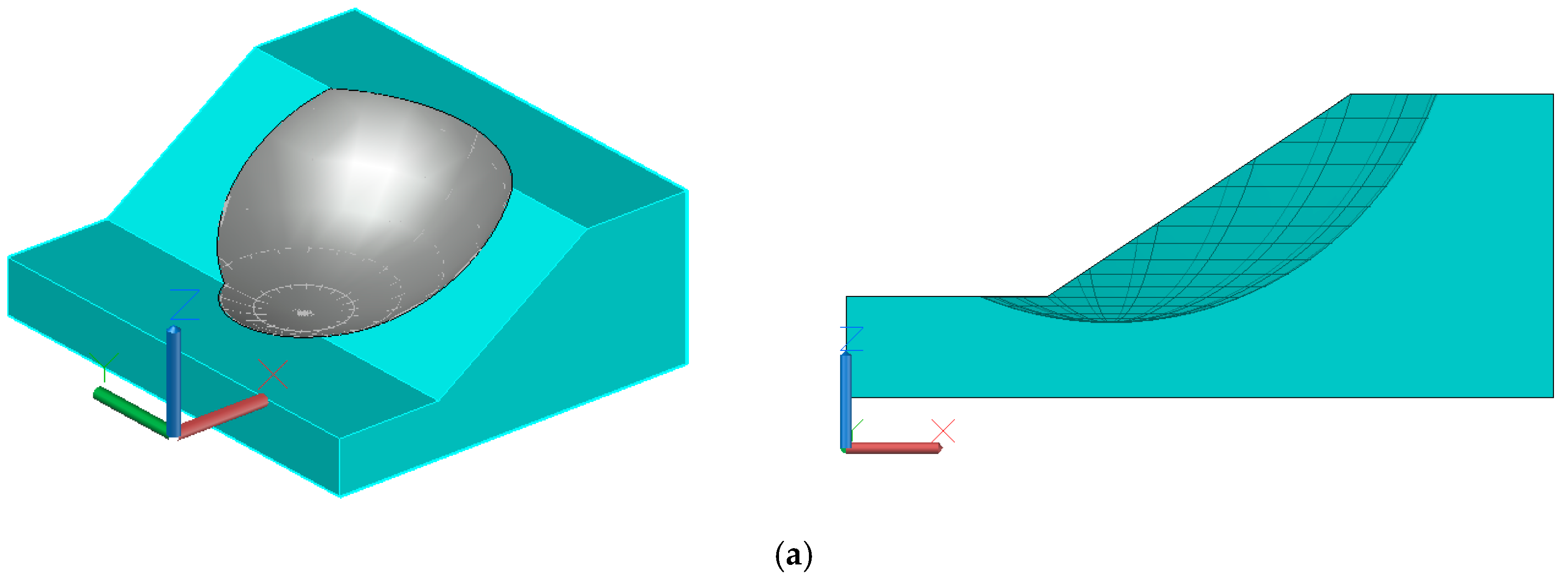
Table 1. The cohesion and internal friction angle of the soil are independent of each other and obey the normal distribution. Considering the two cases with and without seismic force on the slope, K c 0 is 0 and 0.1, respectively. Both sliding surfaces are spherical, and the position and range are shown in Figure 4. The equations are ( x 26.22 ) 2 + y 2 + z 46.86 2 = 34.48 2 (denoted by sliding surface 1, abbreviated as S1) and ( x 29.529 ) 2 + y 2 + z 49.306 2 = 35.667 2 (denoted by sliding surface 2, abbreviated as S2). The results of the six methods are shown in Table 2.
In the case of no seismic load on the slope (i.e., K c 0 = 0.1) and the sliding surface is S1, the calculation results in Tun [8] are taken as the reference values. Among the six methods, the relative errors of the reliability index and failure probability of F s + MCS method are the smallest, while that of the K c + FOSM method is the largest. The relative error of the K c + SS method is the second smallest. Except that the relative error of the failure probability of the K c + FOSM method reaches 22.22%, those of other results are less than 20%. However, the computational efficiency of the six methods is very different. The calculation time of the F s + MCS method is the longest, but it is much less than that in Tun [8]. Both the K c + FOSM and F s + FOSM methods have very short CPU time, even less than 0.5 s. The calculation time of the K c + SS method is slightly less than that of the F s + SS method, which is about half of the K c + MCS method and one-fourth of the F s + MCS method.
When there is a seismic load on the slope (i.e., K c 0 = 0.1) and the slip surface is S2, the failure probability of the 3D slope increases and the reliability index decreases. The results of K c + MCS, K c + SS, and K c + FOSM are very close. The maximum relative errors of the reliability index and failure probability are 3.80% and 7.37%, respectively. In Example 1, the reliability indexes of the 3D slope are slightly higher than that of the 2D slope.
From the above, it can be concluded that the K c performance function can improve the efficiency of the 3D slope reliability analysis without an obvious loss of precision. The method coupled with the SS method can further reduce the amount of calculation.

4.2. Example 2

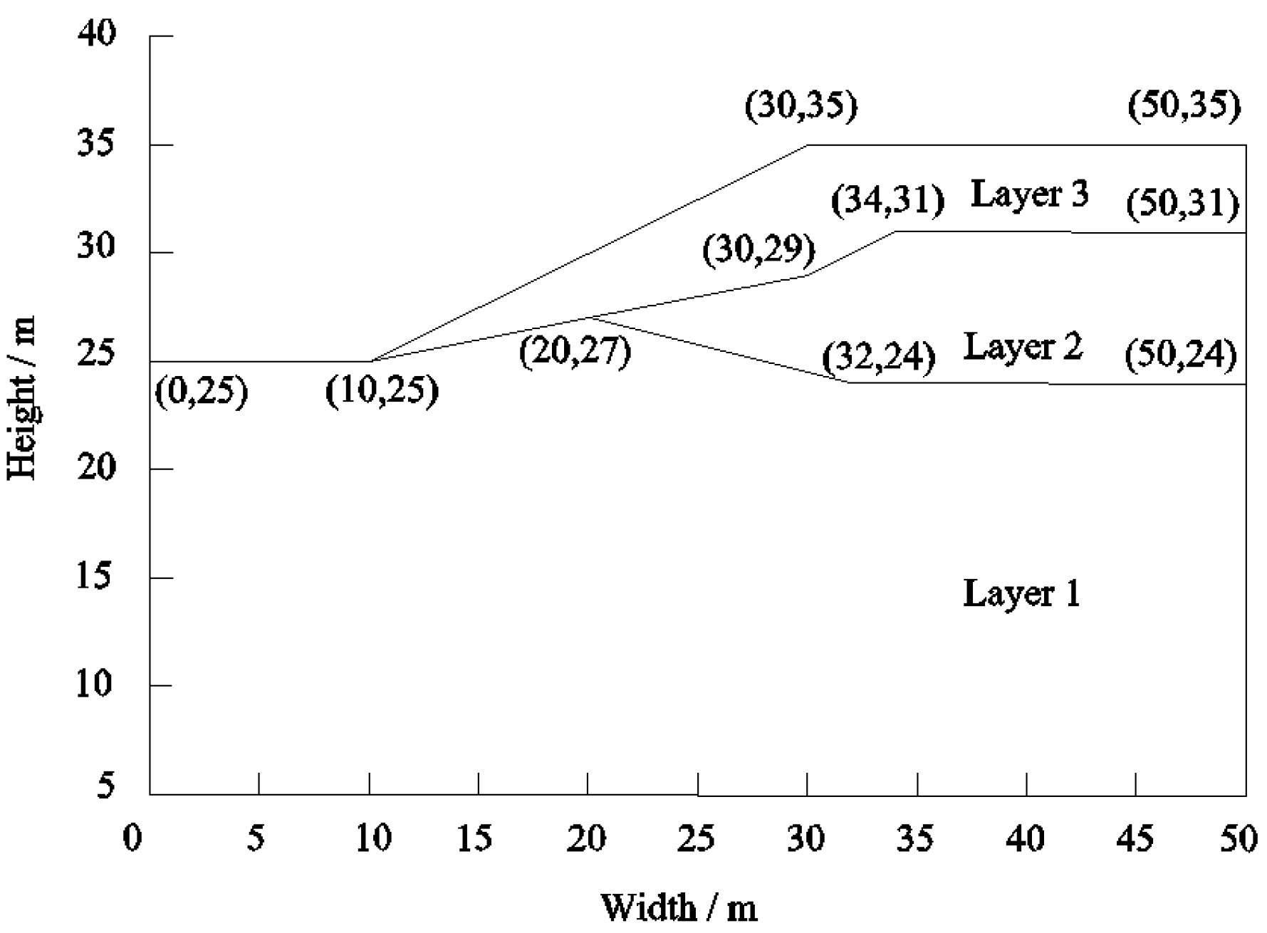
The second example is a slope with three soil layers, which is adapted from a slope stability test question of the Australian Computer Aided Design Association (ASCD) [33]. The distribution of the soil layer in the slope section is shown in Figure 5. The material parameter variables are normally distributed and are listed in Table 3.
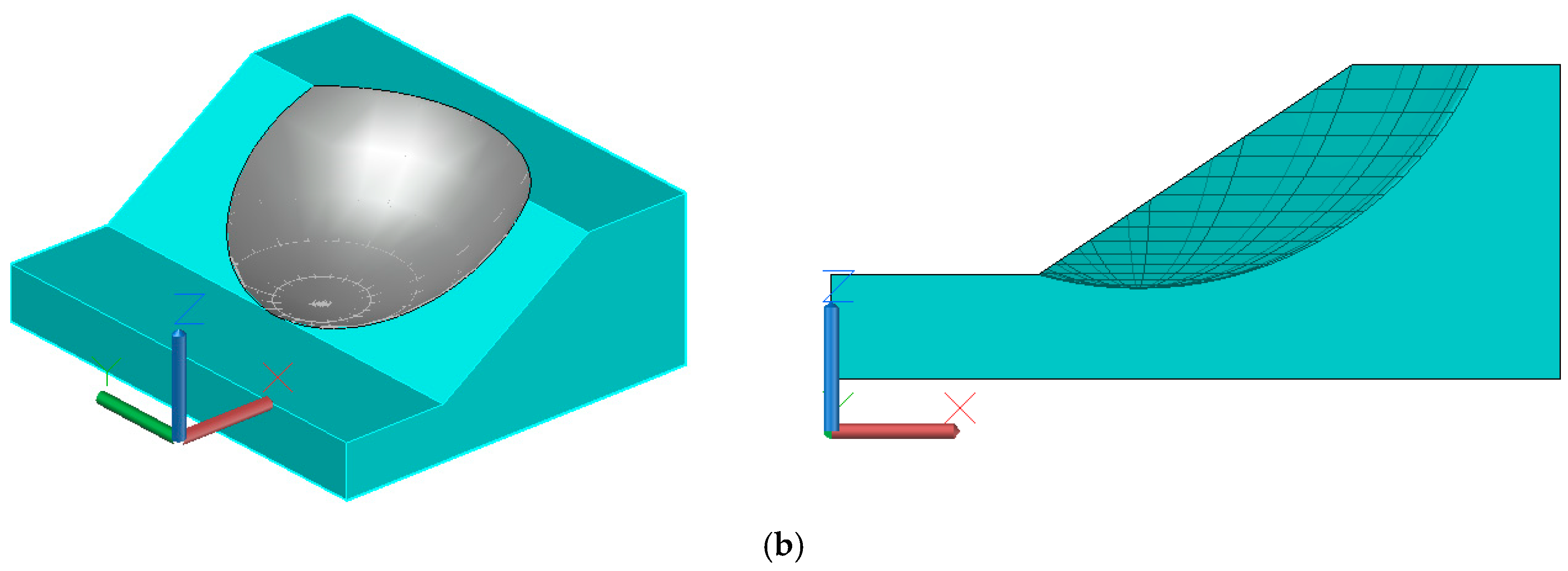
In order to compare with the 2D results, several 3D slope reliability analyses with different lengths are carried out. Firstly, a 3D slope with a spherical sliding surface of 40 m long is designed. Then, keeping the shape of the cross-section of the slope unchanged, the length of the slope is expanded by an integer multiple (the slope length expansion multiple is denoted by η ). The sliding surfaces of long slopes are all ellipsoids, and their longitudinal axis length increases with the slope length. The positions and ranges of two kinds of sliding surfaces are shown in Figure 6. Table 4 lists the results of the 3D slope reliability calculation with different methods under the condition of two kinds of sliding surfaces. The curves of the reliability index and failure probability with slope length are shown in Figure 7.
It can be seen from Table 4 that the failure probability of F s + MCS, K c + MCS, F s + SS, and K c + SS is basically the same as that of Tun [8] in the case of the 3D spherical slip surface, with the maximum relative error of reliability index at less than 5%. The calculated results of F s + FOSM and K c + FOSM are quite different from those of Tun [8], with the maximum relative error of failure probability at more than 50%. In terms of calculation efficiency, the calculation time of the six methods is still very different, but they are far less than that of Tun [8]. Among these methods, the K c + SS method is the one with good calculation accuracy and efficiency.
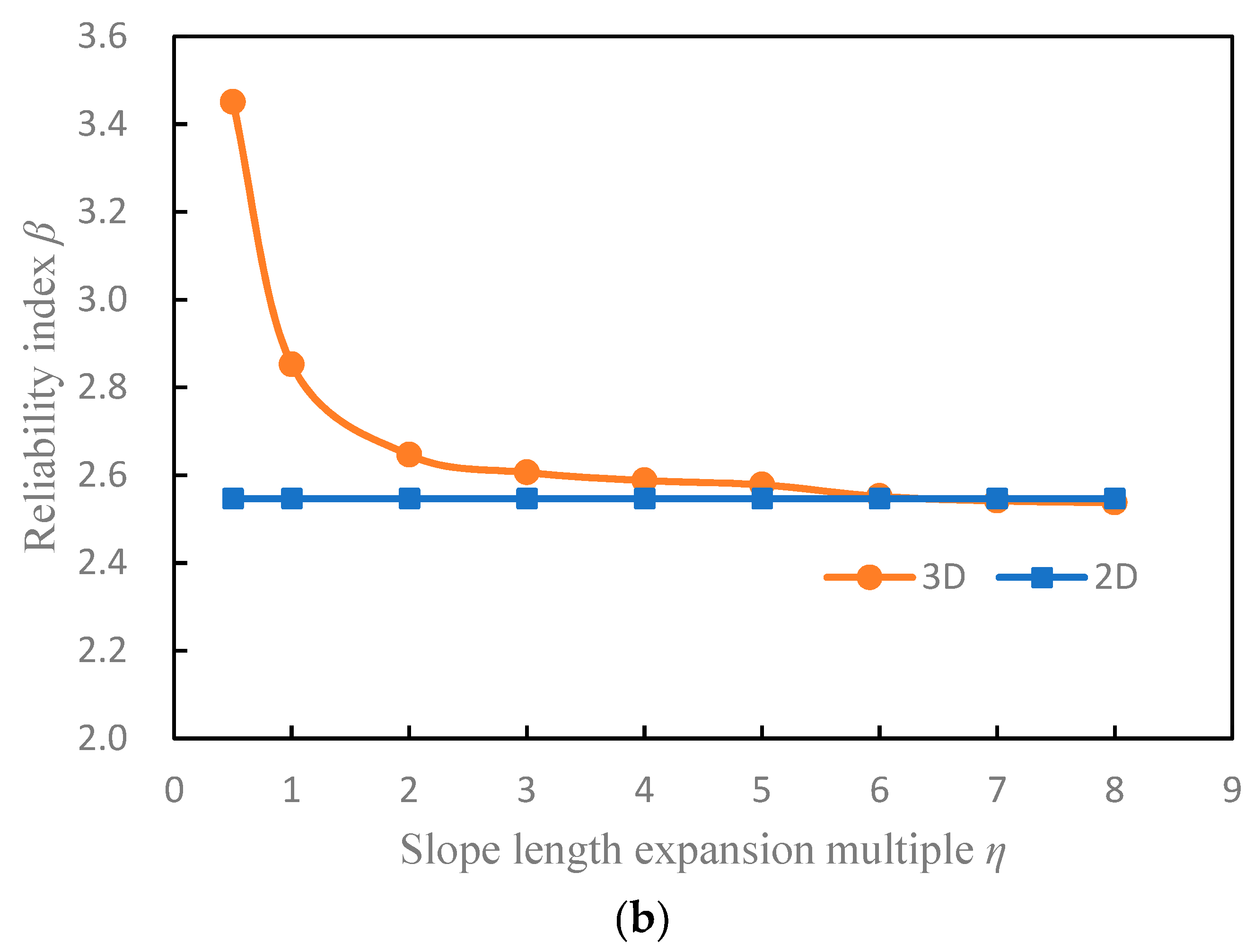
When the slope length is increased by seven times ( η = 7), the failure probabilities of the K c + MCS and K c + SS methods are very close and slightly larger than those of the 2D results. It can be seen that the results of the 2D slope reliability analysis are not always conservative.
Figure 7 shows the trend of increasing failure probability and decreasing reliability index with increasing slope length. When η = 6, the reliability results of the 3D slope are roughly equal to those of the 2D slope. If η is greater than 6, the failure probability of the 3D slope will exceed that of the 2D slope. For the case of long slopes, only the 2D reliability analysis does not necessarily provide a conservative result. It is consistent with the conclusions of Xiao [1] and Qi [34]. It is very necessary to analyze the 3D reliability of the actual long slope.

5. Conclusions

The traditional 3D slope reliability analysis method has low computational efficiency. The reason is that the limit state function is generally expressed by the safety factor, which needs to be solved iteratively. Under the framework of the limit equilibrium method of the 3D slip surface normal stress correction, the critical horizontal acceleration coefficient K c is used as an alternative to the safety factor F s to measure the stability of the slope. Coupled with the reliability algorithm, a simplified method for calculating the reliability of the 3D slope is proposed.
By studying two 3D slope examples, the following conclusions can be drawn:
(1)
This method has the advantages of simple calculation, no iterative convergence problem, and high calculation efficiency. Combined with the SS method, it can fully reflect the advantages of high accuracy and efficiency.
(2)
By changing K c 0 to a value greater than zero, this method can conveniently calculate 3D slope reliability under seismic loads without large-scale modification of the calculation program.
(3)
In the case of a long slope, the results of 2D reliability calculation do not necessarily underestimate the stability of the slope, so it is necessary to carry out 3D slope reliability analysis.
This method only considers the force balance in three directions and moment balance in the y-axis direction and does not belong to the rigorous 3D limit equilibrium method. However, the quasi-rigorous solution is very close to the rigorous solution, and the difference can be ignored. At present, the spatial variability of soil parameters and the influence of groundwater on the reliability of 3D slopes are not considered in this method. Especially, the variability of soil parameters in the direction of slope length will make the results of 3D slope reliability analysis significantly different from those of the 2D slope. That will be the focus of the next research work on this method. In addition, on the basis of this method and a large number of practical 3D slope reliability studies, the design charts can be made for designers to use conveniently, which can improve the practical application value of this method.

Author Contributions

Conceptualization, J.C. and D.Z.; methodology, J.C. and D.Z.; software, J.C.; validation, D.Z. and Y.Z.; formal analysis, J.C., D.Z. and Y.Z.; investigation, J.C.; data curation, J.C.; writing—original draft preparation, J.C.; writing—review and editing, J.C., D.Z. and Y.Z.; visualization, J.C. All authors have read and agreed to the published version of the manuscript.

Funding

This work was funded by the National Natural Science Foundation of China (NSFC Grant No. 52079121).

Data Availability Statement

The data supporting the findings of this study are not publicly available due to privacy.

Conflicts of Interest

The authors declare no conflict of interest.

References

  1. Xiao, T.; Li, D.-Q.; Cao, Z.-J.; Au, S.-K.; Phoon, K.-K. Three-dimensional slope reliability and risk assessment using auxiliary random finite element method. Comput. Geotech. 2016, 79, 146–158. [Google Scholar] [CrossRef]
  2. Varkey, D.; Hicks, M.; Vardon, P. An improved semi-analytical method for 3D slope reliability assessments. Comput. Geotech. 2019, 111, 181–190. [Google Scholar] [CrossRef]
  3. Duncan, J.M. Factors of Safety and Reliability in Geotechnical Engineering. J. Geotech. Geoenviron. Eng. 2000, 126, 307–316. [Google Scholar] [CrossRef]
  4. Chen, C.-F.; Xiao, Z.-Y.; Zhang, G.-B. Time-variant reliability analysis of three-dimensional slopes based on Support Vector Machine method. J. Central South Univ. Technol. 2011, 18, 2108–2114. [Google Scholar] [CrossRef]
  5. Al-Jeznawi, D.; Alzabeebee, S.; Shafiqu, Q.S.M.; Güler, E. Analysis of Slope Stabilized with Piles Under Earthquake Excitation. Transp. Infrastruct. Geotechnol. 2022, 1–19. [Google Scholar] [CrossRef]
  6. Tolun, M.; Un, B.; Emirler, B.; Yildiz, A. Stability analyses of a slope reinforced with piles subjected to static and dynamic loading conditions. El-Cezerî J. Sci. Eng. 2021, 8, 1360–1371. [Google Scholar] [CrossRef]
  7. Auvinet, G.; González, J. Three-dimensional reliability analysis of earth slopes. Comput. Geotech. 2000, 26, 247–261. [Google Scholar] [CrossRef]
  8. Tun, Y.W.; Llano-Serna, M.A.; Pedroso, D.M.; Scheuermann, A. Multimodal reliability analysis of 3D slopes with a genetic algorithm. Acta Geotech. 2019, 14, 207–223. [Google Scholar] [CrossRef]
  9. Cheng, Y.M.; Li, L.; Liu, L.L. Simplified approach for locating the critical probabilistic slip surface in limit equilibrium analysis. Nat. Hazards Earth Syst. Sci. 2015, 15, 2241–2256. [Google Scholar] [CrossRef]
  10. Xiao, S.; Zeng, J.; Yan, Y. A rational layout of double-row stabilizing piles for large-scale landslide control. Bull. Eng. Geol. Environ. 2017, 76, 309–321. [Google Scholar] [CrossRef]
  11. Tang, H.; Hu, X.; Xu, C.; Li, C.; Yong, R.; Wang, L. A novel approach for determining landslide pushing force based on landslide-pile interactions. Eng. Geol. 2014, 182, 15–24. [Google Scholar] [CrossRef]
  12. Vanmarcke, E.H. Reliability of Earth Slopes. J. Geotech. Eng. Div. 1977, 103, 1247–1265. [Google Scholar] [CrossRef]
  13. Zhang, W.-S.; Luo, Q.; Jiang, L.-W.; Wang, T.-F.; Tang, C.; Li, Z.-T. Improved Vanmarcke analytical model for 3D slope reliability analysis. Comput. Geotech. 2021, 134, 104106. [Google Scholar] [CrossRef]
  14. Hicks, M.; Spencer, W. Influence of heterogeneity on the reliability and failure of a long 3D slope. Comput. Geotech. 2010, 37, 948–955. [Google Scholar] [CrossRef]
  15. Xu, Z.-X.; Zhou, X.-P. Three-dimensional reliability analysis of seismic slopes using the copula-based sampling method. Eng. Geol. 2018, 242, 81–91. [Google Scholar] [CrossRef]
  16. Shu, S.; Ge, B.; Wu, Y.; Zhang, F. Probabilistic Assessment on 3D Stability and Failure Mechanism of Undrained Slopes Based on the Kinematic Approach of Limit Analysis. Int. J. Geomech. 2023, 23, 06022037. [Google Scholar] [CrossRef]
  17. Cho, S. Probabilistic assessment of slope stability that considers the spatial variability of soil properties. J. Geotech. Geoenviron. Eng. 2010, 136, 975–984. [Google Scholar] [CrossRef]
  18. Hungr, O.; Salgado, F.M.; Byrne, P.M. Evaluation of a three-dimensional method of slope stability analysis. Can. Geotech. J. 1989, 26, 679–686. [Google Scholar] [CrossRef]
  19. Huang, C.-C.; Tsai, C.-C.; Chen, Y.-H. Generalized Method for Three-Dimensional Slope Stability Analysis. J. Geotech. Geoenviron. Eng. 2002, 128, 836–848. [Google Scholar] [CrossRef]
  20. Chen, Z.; Mi, H.; Zhang, F.; Wang, X. A simplified method for 3D slope stability analysis. Can. Geotech. J. 2003, 40, 675–683. [Google Scholar] [CrossRef]
  21. Zhou, X.; Cheng, H. Stability analysis of three-dimensional seismic landslides using the rigorous limit equilibrium method. Eng. Geol. 2014, 174, 87–102. [Google Scholar] [CrossRef]
  22. Kasama, K.; Furukawa, Z.; Hu, L. Practical reliability analysis for earthquake-induced 3D landslide using stochastic response surface method. Comput. Geotech. 2021, 137, 104303. [Google Scholar] [CrossRef]
  23. Song, L.; Xu, B.; Kong, X.; Zou, D.; Yu, X.; Pang, R. Reliability Analysis of 3D Rockfill Dam Slope Stability Based on the Copula Function. Int. J. Géoméch. 2021, 21, 04021001. [Google Scholar] [CrossRef]
  24. Sarma, S.K. Stability analysis of embankments and slopes. Géotechnique 1973, 23, 423–433. [Google Scholar] [CrossRef]
  25. Zhu, D.; Qian, Q. Rigorous and quasi-rigorous limit equilibrium solutions of 3D slope stability and application to engineering. Chin. J. Rock Mech Eng. 2007, 26, 1513–1528. [Google Scholar] [CrossRef]
  26. Au, S.; Wang, Y. Engineering Risk Assessment with Subset Simulation; John Wiley & Sons: Singapore, 2014; pp. 157–202. [Google Scholar] [CrossRef]
  27. Chen, J.; Zhu, D.; Zhu, Y. An efficient method for computing slope reliability calculation based on rigorous limit equilibrium. Appl. Rheol. 2023, 33, 20220147. [Google Scholar] [CrossRef]
  28. Hovland, H.J. Three-Dimensional Slope Stability Analysis Method. J. Geotech. Eng. Div. 1977, 103, 971–986. [Google Scholar] [CrossRef]
  29. Sarma, S. Stability analysis of embankments and slopes. Journal of Geotechnical and Geoenvironmental Engineering Division. ASCE 1979, 105, 1511–1524. [Google Scholar] [CrossRef]
  30. Halatchev, R. Probabilistic stability analysis of embankments and slopes. In Proceedings of the 11th International Conference on Ground Control in Mining, Wollongong, NSW, Australia, 7–10 July 1992. [Google Scholar]
  31. Zhu, Y. Slope Reliability Analysis; Metallurgical Industry Press: Beijing, China, 1993; pp. 218–274. [Google Scholar]
  32. Arai, K.; Tagyo, K. Determination of Noncircular Slip Surface Giving the Minimum Factor of Safety in Slope Stability Analysis. Soils Found. 1985, 25, 43–51. [Google Scholar] [CrossRef]
  33. Ji, J.; Low, B.K. Stratified Response Surfaces for System Probabilistic Evaluation of Slopes. J. Geotech. Geoenviron. Eng. 2012, 138, 1398–1406. [Google Scholar] [CrossRef]
  34. Qi, S.; Ling, D.; Yao, Q.; Lu, G.; Yang, X.; Zhou, J.-W. Evaluating slope stability with 3D limit equilibrium technique and its application to landfill in China. Eng. Geol. 2021, 280, 105939. [Google Scholar] [CrossRef]
Figure 1. Three-dimensional slope, soil column, and forces. (a) Three-dimensional slope and sliding body. (b) Soil column and forces.
Water 15 03139 g001
Figure 2. The relation curve of F s and K .
Water 15 03139 g002
Figure 3. Cross-section of homogeneous slope in Example 1.
Water 15 03139 g003
Figure 4. The sliding surface position and range of Example 1. (a) Three-dimensional slip surface at K c 0 = 0 . (b) Three-dimensional slip surface at K c 0 = 0.1 .
Water 15 03139 g004aWater 15 03139 g004b
Figure 5. Cross-section of three-layer slope in Example 2.
Water 15 03139 g005
Figure 6. The slip surface position and range of the three-layer slope in Example 2. (a) Three-dimensional sphere slip surface. (b) Three-dimensional ellipsoid slip surface.
Water 15 03139 g006
Figure 7. Relationship curves between reliability results and slope length. (a) The curve of failure probability with slope length. (b) The curve of reliability index with slope length.
Water 15 03139 g007aWater 15 03139 g007b
Table 1. Material parameters of the slope in Example 1.
Cohesion   c (kPa) Friction   Angle   φ (°) Unit   Weight   γ (kN/m3)
μ c σ c μ ϕ σ ϕ
41.658.0015.003.0018.82
Table 2. Comparison of reliability analysis results of Example 1.
Performance
Functions
Reliability Methods Horizontal   Seismic   Coefficient   K c 0 Sampling   Number   N β P f Slip Surface Shape Computation   Time   t (s)
F s methodMCS040,0002.63760.00423D S121.70
K c methodMCS040,0002.66060.00393D S112.45
F s methodSS040,0002.67800.00373D S16.80
K c methodSS040,0002.64380.00413D S15.45
F s methodFOSM0 2.65960.00393D S10.30
K c methodFOSM0 2.69370.00353D S10.13
BishopGA + FORM0 2.61000.0045 [8]3D S1>3.8 h
Bishop (GeoStudio)MCS040,0002.24220.01202D circular S1
K c methodMCS0.140,0001.83170.03353D S212.98
K c methodSS0.140,0001.86330.03123D S25.33
K c methodFOSM0.1 1.84320.03263D S20.14
Bishop (GeoStudio)MCS0.140,0001.18700.11762D circular S2
MCS—Monte Carlo simulation; SS—subset simulation; GA—genetic algorithm; FORM—first-order reliability method; FOSM—first-order second-moment method.
Table 3. Material parameters of the slope in Example 2.
Soil Layer Cohesion   c (kPa) Friction   Angle   φ (°) Unit   Weight   γ (kN/m3)
μ c σ c μ ϕ σ ϕ
Layer 100380.119.5
Layer 25.30.53234.619.5
Layer 37.21.44204.019.5
Table 4. Results of reliability analysis of Example 2 by different methods.
Performance
Functions
Reliability Methods Sampling   Number   N β P f Slip Surface Shape Computation   Time   t (s)
F s methodMCS100,0002.85760.00213D sphere58.98
K c methodMCS100,0002.88940.00193D sphere31.48
F s methodSS100,0002.86820.00213D sphere18.23
K c methodSS100,0002.87070.00203D sphere16.89
F s methodFOSM 2.74110.00313D sphere0.80
K c methodFOSM 2.71520.00333D sphere0.44
BishopGA + FORM 2.89000.0019 [8]3D sphere~7 h
K c methodMCS100,0002.54140.00553D ellipsoid ( η = 7)163.59
K c methodSS100,0002.53600.00563D ellipsoid ( η = 7)56.92
K c methodFOSM 2.42900.00763D ellipsoid ( η = 7)0.61
Bishop (GeoStudio)MCS100,0002.54650.00542D circular
MCS—Monte Carlo simulation; SS—subset simulation; GA—genetic algorithm; FORM—first-order reliability method; FOSM—first-order second-moment method.
Disclaimer/Publisher’s Note: The statements, opinions and data contained in all publications are solely those of the individual author(s) and contributor(s) and not of MDPI and/or the editor(s). MDPI and/or the editor(s) disclaim responsibility for any injury to people or property resulting from any ideas, methods, instructions or products referred to in the content.

