Article

Evaluation of Methods for Estimating Long-Term Flow Fluctuations Using Frequency Characteristics from Wavelet Analysis

1
Department of Civil and Environmental Engineering, University of Hawaii at Manoa, Honolulu, HI 96822, USA
2
Department of Environment and Forest Resources, Chungnam National University, Daejeon 34134, Republic of Korea
3
Department of Civil Engineering, Seoul National University of Science and Technology, Seoul 01811, Republic of Korea
4
Department of Civil and Environmental Engineering, Chung-Ang University, Seoul 06974, Republic of Korea
*
Author to whom correspondence should be addressed.
Water 2023, 15(16), 2968; https://doi.org/10.3390/w15162968
Submission received: 22 July 2023 / Revised: 12 August 2023 / Accepted: 15 August 2023 / Published: 17 August 2023

Abstract

:
This study was aimed at exploring different indices to quantify flow fluctuations and calculate long-term flow indicators (L-FFI). Three approaches were considered to calculate the indicators: Method (1)—calculate the annual index and then average it; Method (2)—average the annual flow characteristics and then calculate the index; and Method (3)—calculate the index considering all available data. Wavelet analysis was performed to evaluate the derived L-FFI. The evaluation index was based on the period corresponding to the highest spectral power from the wavelet transformation of seasonally differenced data. Strong and negative positive correlations were observed between the L-FFI and the high- and low-flow variations, respectively. The correlation coefficient ( R ) between L-FFIs and the frequency with maximum global wavelet power showed that Method (2) consistently yielded the most reliable results across various facets, having a determination coefficient of 0.73 ( R 2 ) on average. In the regionalization analysis using the Ward method, it was consistently observed that the two largest dams (the Chungju Dam and the Uiam Dam) were significantly differentiated from the other dams. Furthermore, Method (2) showed the most similar characteristics to the clustering of the wavelet features. The outcomes are expected to facilitate long-term water resource management.

1. Introduction

A notable characteristic of climate in Korea is that the rainfall is concentrated in the summer season, which leads to significant variations in the flow discharge in a short period. These flow fluctuations are closely related to the hydrological and ecological stability of rivers. In addition, flow fluctuations considerably influence the efficiency of water resource utilization and pose potential risks associated with flooding. Therefore, it is necessary to examine the long-term flow variability for a specific basin (or watershed), and considerable research has been focused on flow fluctuations [1,2,3,4,5].
Various indices are available for quantifying the variability in flow fluctuations. A representative flow fluctuation index (FFI) is the river regime coefficient (RRC), which is the ratio of the maximum flow discharge to the minimum flow discharge in a certain period. Several researchers have focused on the RRC in the Korean environment. Won [6] estimated the RRC based on flow discharge data of the five major river basins in Korea in the 1920s. Later, Park [7] estimated the RRC using flow discharge data of the Geum river in Korea. Lee and Woo [8] and Lee et al. [9] estimated the RRC using flow discharge data of the major five rivers in Korea, similar to [6].
In the 2000s, several researchers examined the indices for various flow fluctuation characteristics. Lee [10] analyzed the flow variability of the Han and Nakdong rivers from 1999 to 2001. Unlike the previous studies, Lee [10] considered not only the maximum and minimum flow but also indices based on ordinary discharge, low discharge, and drought discharge. Subsequently, Handayani [11] estimated the annual RRCs from 2006 to 2015 based on discharge data from the Rokan river in Sumatra, Indonesia, where flood damage frequently occurs, and analyzed the temporal variations in the RRCs. Unlike [10], who focused on a multi-year period, Handayani [11] set the analysis period as one year. Overall, different researchers have used different methods to calculate long-term indices, leading to a certain subjectivity in the findings. Although the indices vary depending on the target period, to the best of our knowledge, none of the existing studies have investigated the variation in the long-term FFI (L-FFI) indices according to the target period or estimation method.
The wavelet analysis technique is commonly used for examining periodic properties and has proven to be an effective tool for time series analyses across various academic fields [12]. Numerous instances of its application can be found in hydrology and meteorology [13,14,15,16,17]. Moreover, recent research has focused on integrating the frequency characteristics obtained through wavelet analysis with machine learning for prediction or forecasting, and promising results have been obtained [18,19,20,21]. Some studies have confirmed the validity of using wavelet analysis to analyze the patterns of dam inflow and river outflow [22,23,24]. Thus, the frequency characteristics derived from wavelet analysis, which are closely related to the flow fluctuations, could serve as an evaluation criterion for assessing L-FFI.
On the other hand, there have been studies related to regionalization, which clusters basins by identifying and interpreting patterns inherent in hydrological features such as these flow characteristics. Most studies have utilized this for regional flood frequency analysis. Cluster analysis methods are predominantly used for regionalization. These can be broadly divided into hierarchical algorithms and partitioning algorithms. A representative method for hierarchical algorithms is Ward’s method [25], and for partitioning algorithms K-means [26] can be mentioned. Hybrid algorithms, which combine these algorithms, are also frequently employed. Various attempts continue to be made to advance hydrological regionalization up to recent times [27,28,29,30,31,32,33]. If such regionalization from L-FFI and wavelet analysis is further conducted, then its applicability in long-term water resource management could be significantly enhanced.
In this study, we evaluated several methods for estimating L-FFI based on the characteristics exhibited by long-term data in the time–frequency domain. While there have been studies that aimed to obtain flow characteristics through flow-related indices or wavelet analysis, research that seeks to integrate both is a novel endeavor. To this end, we first investigated the indices for quantifying the flow fluctuations, considering three methods for estimating the L-FFI. The frequency characteristics were defined using the frequency with the highest spectral power from the result of the wavelet transformation of seasonally differenced data. The methods for L-FFI were evaluated based on these frequency characteristics. Furthermore, based on the results of the L-FFI and frequency characteristics, we conducted regionalization of the dam basin using hierarchical clustering with the Ward algorithm and discuss the implications.

2. Materials and Methods

2.1. Study Area and Data

The study objects were eight domestic dam basins, for which long-term inflow data were extracted. We selected basins that are not significantly affected by upstream hydraulic structures. The analysis period encompassed 36 years, from 1986 to 2021. Daily discharge data for the dam basins were obtained through the daily inflow data provided by the Water Resources Management Information System (http://www.wamis.go.kr, accessed on 1 April 2023) in Korea. Figure 1 shows the considered basins, river networks, and dam locations. Table 1 summarizes the basic information of the dam and dam basin.

2.2. FFI

The RRC is a representative index for quantifying flow fluctuations. Additionally, specific flow characteristics based on discharge that occurs for more than a specific number of days in a year (i.e., daily discharge occurring in a specific order throughout the year) can be used for evaluation. This parameter, known as the flow regime, is commonly used in hydrological research [34]. In this study, periods of 10, 95, 185, 275, and 355 d were selected, corresponding to flood discharge, abundant discharge, ordinary discharge, low discharge, and drought discharge, respectively. Such discharges are typically expressed as exceedance probabilities. Thus, the discharges considered in this study corresponded to exceedance probabilities of 2.7%, 26.0%, 50.7%, 75.3%, and 97.3%, defined as Q 2.7 , Q 26.0 , Q 50.7 , Q 75.3 , and Q 97.3 , respectively.
The RRC can be formulated as follows:
R R C = Q max / Q min
where Q max and Q min denote the maximum and minimum discharge at a specific point in the stream in a specific period, respectively. In estimating the RRC, the target period has been set as the specific period by various researchers. For example, Lee and Woo [8] estimated the RRC for several decades before and after the construction of five major dams in Korea to evaluate the change in the RRC owing to the dam construction. The average value of the RRCs within the long-term period was considered for calculating the long-term RRC. Lee [10] compared the changes in the annual RRC in Korea using daily discharge data from 1999 to 2001, for which a substantial amount of discharge data were available compared with those in the other periods. In contrast, certain researchers considered a period spanning several decades, depending on the objective for estimating the RRC.
Because the RRC is sensitive to extreme discharge values observed during drought or flood periods, it cannot effectively reflect the variations in the average flow fluctuations. A promising alternative is the flow regime coefficient ( C R ) [9], expressed as
C R = Q 2.7 / Q 97.3
Although the meaning of this coefficient is similar to that of the RRC, it can overcome the abovementioned limitation of the RRC.
In addition, Park [35] proposed the flood coefficient ( C F ) and abundance coefficient ( C A ) to quantify the flow fluctuations above the ordinary discharge ( Q 50.7 ):
C F = Q max / Q 50.7
C A = Q 26.0 / Q 50.7
where C F and C A exceed 1. Smaller values of the coefficients indicate a higher similarity of Q max and Q 26.0 to Q 50.7 , i.e., reduced flow fluctuations above the ordinary discharge.
Considering that there may be a difference in the flow fluctuations above or below the ordinary discharge, Park [35] proposed a low coefficient ( C L ) and drought coefficient ( C D ), expressed as
C L = Q 75.3 / Q 50.7
C D = Q 97.3 / Q 50.7
where C L and C D are smaller than 1, and as their value increases, the values of Q 75.3 and Q 97.3 approach that of Q 50.7 . In other words, the flow fluctuations of the river decrease.
Furthermore, Park [36] investigated the flow fluctuations based on abundant discharge. The ratio of C A to C D and that of C A to C L were defined as the variance of the drought coefficient ( C V D ) and the variance low coefficient ( C V L ), respectively.
C V D = C A / C D = Q 26.0 / Q 97.3
C V L = C A / C L = Q 26.0 / Q 75.3
Additionally, we considered the coefficient of variance ( C V ), which is widely used in various fields. C V , also known as the relative standard deviation, can be used for comparing variables with different absolute scales. In this study, in addition to the commonly used mean values, we considered the index based on median values. The two indices are distinguished by the subscripts:
C V μ = Q σ / Q μ
C V m = Q σ / Q m
where Q μ and Q m denote the average discharge (m3/s) and median discharge (m3/s), respectively. Q σ is the standard deviation (m3/s). C V μ and C V m are the coefficients of variation based on Q μ and Q m , respectively. Table 2 summarizes the FFIs mentioned earlier and provides a brief description of each.

2.3. Wavelet Transform

There are various methods to analyze signals in the time domain; for example, ARIMA (auto regressive integrated moving average) [37], exponential smoothing [38], SSM (state space models) [39,40], VAR (vector autoregressions) [41], decomposition [42,43], approximation of differential equations [44,45], etc. Among them, conventionally, Fourier transformations have been widely used to analyze signals in the time domain by transforming them to the frequency domain [46,47]. As the Fourier transform uses sine and cosine functions as the basis functions, it is particularly useful in analyzing the overall periodicity rather than local changes. However, if the time series data are non-stationary, the periodic characteristics may not be consistent throughout the data period. This problem is commonly encountered with most time series data observed in nature. To overcome this limitation, the concept of time–frequency analysis has been introduced [48,49]. Time–frequency analysis based on Fourier transform shows the variation in the relative importance of the sine or cosine function at each time point.
Although time–frequency analyses based on Fourier transformations represent a valuable tool, they involve several limitations. The most fundamental limitation is that the basis functions repeat indefinitely, which means that their influence extends across the entire time series. In examining the frequency characteristics of long-term time series data, as in this study, one could potentially apply Fourier analysis. However, in such instances, it becomes challenging to clarify temporal changes in the frequency variations.
The wavelet analysis technique was established to overcome this drawback [50,51]. A wavelet refers to a small wave that has a finite length. Thus, wavelet transformations use basis functions of finite length to transform the existing time series data into the time–frequency domain. Compared with Fourier transformations, wavelet transformations can more clearly represent local changes, which is beneficial for identifying discontinuous points in signals.
The basis function of the wavelet transform is known as the mother wavelet. By the scaling and transition of the mother wavelet, signals in the time domain can be transformed to the frequency domain. For a time series x t , the continuous wavelet transform (CWT) is calculated as shown in (11).
W x a ,   b = 1 a x ( t ) ψ * t b a d t
where W x a ,   b represents the CWT with parameters a and b , where a is the scale parameter that adjusts the size of the mother wavelet, and b is the transition parameter that shifts the position of the mother wavelet along the time axis. ψ * denotes the mother wavelet function, and the superscript * represents the complex conjugate. The W x a ,   b computed from (10) typically takes complex values, and thus, to perform comparisons based on magnitudes, the wavelet power (WP) computed as W x a ,   b 2 is commonly used. The average WP over the entire period is referred to as the global WP (GWP).
The mother wavelet must be carefully selected considering the research objective, as it considerably affects the results of wavelet analysis even when using the same data [52]. Furthermore, if an inappropriate mother wavelet is chosen, a problem with convergence could be encountered. In univariate mother wavelet analysis, the Morlet mother wavelet yields consistent results in both the time and frequency domains compared with other mother wavelets [53,54,55,56]. Therefore, the analysis in this study was based on the Morlet mother wavelet, which can be expressed as in (2).
ψ η = π 1 / 4 e i ω 0 η e η 2 / 2
where η represents the non-dimensional time parameter transformed by the scale and transition parameters. ω 0 is the wave number, which is also referred to as the non-dimensional frequency, set as 6 in this study. In these settings, the Morlet mother wavelet generates six oscillations. Furthermore, setting ω 0 as 6 has been known to provide the optimal balance in terms of localization in the time–frequency domain during the wavelet transformation [53,54,55,56].
After determining the mother wavelet, the frequency to be analyzed must be set. Typically, this setting is defined using the scale, which is the reciprocal of the frequency. The scale is determined using (13), and J, which denotes the index of the largest scale, is obtained through (14) [57].
s j = s 0 2 j δ j ,         j = 0 ,   1 ,   ,   J
J = δ j 1 log 2 N δ t / s 0
where s j represents the scale size at j , and j denotes the index of the scale, ranging from 0 to J . Therefore, the total number of scales to be analyzed is J + 1 . s 0 is the smallest value among the scales to be analyzed, and δ j determines the density of the scale. δ j is a constant and setting it to a smaller value enables a more precise representation of the wavelet spectrum. Typically, δ j is set as 0.4875 [51]. However, its value is set as 0.25 in this study to obtain finer details. δ t is the time unit for wavelet analysis. The small scale ( s 0 ) is generally set as 2 δ t .
Compared with Fourier transformations, the wavelet transformation, which converts data from the time domain into the time–frequency domain, yields less straightforward interpretations. The frequency displayed in the time–frequency domain by the wavelet spectrum may not necessarily represent the frequency of the original data. The same problem is encountered with the scale, which is inversely proportional to the frequency. This discrepancy arises because unlike Fourier transformation, which uses sine or cosine functions of a certain frequency as the basis functions, the center frequency of the mother wavelet used as the basis function in wavelet analysis differs for each function. Nevertheless, when the Morlet mother wavelet ( m = 6 ) is used, the frequency observed in the wavelet analysis closely approximates the frequency of the original data ( λ s = 1.03   s ), which enhances the interpretability of the results.
Additionally, the results of wavelet analysis typically include an area known as the cone of influence (COI) in which edge effects cannot be ignored. Caution must be exercised when interpreting results within this area due to its high uncertainty. When using the Morlet mother wavelet, the COI at scale s is calculated as 2 s [53]. We used the Python package PyCWT, and the code was developed with reference to the work of [57].

2.4. Regionalization of Basins

Regionalization of basins is primarily a method utilized for regional flood frequency analysis (RFFA). When the flood records of a specific basin are very short, it involves grouping basins that have hydrological homogeneity in the vicinity, and then conducting FFA based on this. Cluster analysis methods are predominantly used for regionalization. These can be broadly divided into hierarchical algorithms and partitioning algorithms. A representative method of hierarchical algorithms is Ward’s method [25], and for partitioning algorithms, K-means [26] can be cited.
In this study, the Ward algorithm, the most basic form of hierarchical algorithms, was employed for regionalization based on the final L-FFI and wavelet analysis results. The Ward algorithm has been successfully applied in previous related studies [58,59,60,61]. An explanation for this is provided as follows:
Firstly, Ward’s algorithm aims to minimize the total variance within the cluster. To implement this method, one must find the pair of clusters at each stage that, when merged, results in the smallest increase in the total intra-cluster variance. Essentially, this measures the similarity of clusters based on the increase in the error sum of squares when two clusters are combined. Thus, in data with m variables, if there are K clusters at the current stage, and each cluster contains N k data, the objective function is expressed as follows:
W = k = 1 K j = 1 m i = 1 N k x i j k x ¯ j k 2
where x i j k represents the value of the i th observation for the j th value in cluster k , and x ¯ j k denotes the average value of the j th value in cluster k .
Thus, the objective function of the Ward algorithm minimizes the sum of squared deviations of feature vectors from each cluster’s center [62]. The Ward algorithm begins with singleton clusters. At this point, the cluster center is identical to the feature vector, and the objective function is computed as zero. At each step of the analysis, the union of all possible pairs of clusters is considered, and the two clusters resulting in the smallest increase in W when merged are combined. Due to merging, the change in the objective function value, W , relies only on the relationship between the two merged clusters and is not influenced by other clusters. Ward’s algorithm is adept at restoring cluster structures and tends to form spherical clusters of equal sizes. These characteristics of the Ward algorithm prove beneficial for identifying similar regions for regionalization [63].

3. Results

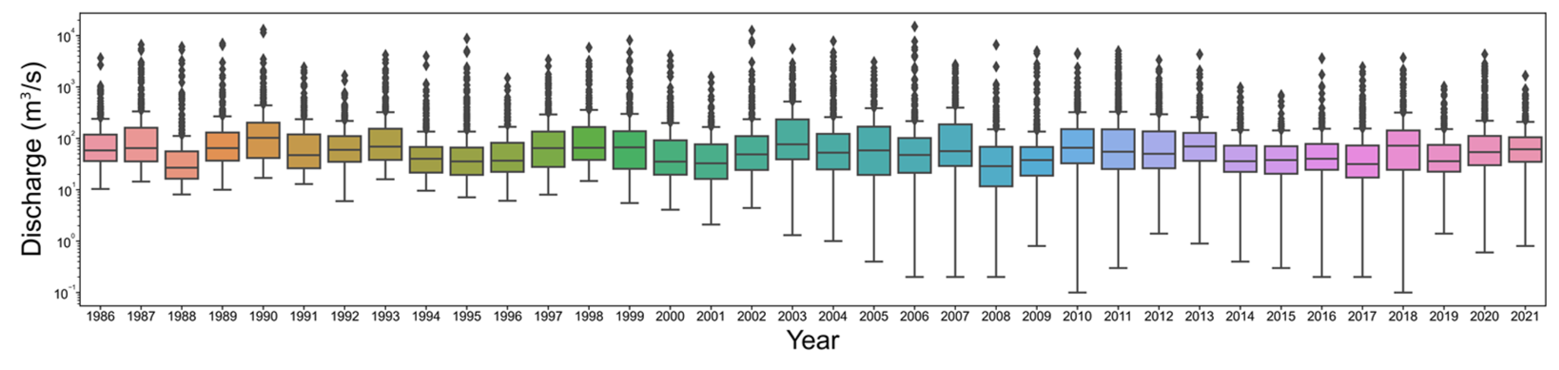
3.1. Pre-Analysis and Estimation of FFI and L-FFI

The existing studies used different periods to estimate the FFIs, such as a single year or multiple years. A standard method for estimating the L-FFIs remains to be established. Therefore, in this study, we evaluated three methods for estimating the L-FFIs for the Chungju Dam basin: Method (1)—average the annual FFIs; Method (2)—calculate the L-FFIs after averaging the annual flow characteristics; and Method (3)—calculate the L-FFIs using the flow characteristics for the entire period.
Figure 2 shows the time series of daily inflow data and the mass curve of the Chungju Dam. Given the large difference in the scale of each year, the horizontal axis is set as a log scale. Although certain differences can be observed among the years, the inflow is generally concentrated in the summer, and the fluctuations vary across the years. In regions such as South Korea, where there is a concentrated rainfall and inflow during specific periods of the year, understanding the variability of dam inflow through metrics such as FFI is crucial from a water resource management perspective. For instance, in areas with high inflow fluctuations, there might be a need to release a significant amount of water for flood prevention, which could subsequently lead to an inability to adequately supply water during drought periods. Conversely, in regions with fewer inflow fluctuations, there is a higher likelihood of efficiently addressing water demands during droughts.
Before diving into the in-depth analysis, we first examined the precipitation patterns. For easier comparison, it is displayed in a log-scale, consistent with previous analyses as shown in Figure 3. Upon examining the correlation coefficient between precipitation and inflow time series, as well as the cross-correlation coefficient with a given lag, it is observed that the correlation coefficient is merely about 0.473 when there is no lag. However, it peaks at 0.716 when a lag of 1 day is given, and then exponentially decreases thereafter. This indicates that the precipitation and inflow time series exhibit similar patterns, with the highest correlation observed at a 1-day lag for the Chungju Dam. Other dams also showed similar characteristics.
Before examining the results for all the dam basins, the results of the Chungju Dam were analyzed. First, the annual flow characteristics were calculated from the daily inflow. Figure 4 shows the flow characteristics in terms of the minimum and maximum daily discharge and major discharge by year for a period of 36 years from 1986 to 2021. Additionally, Figure 5 displays the box-plot of the annual inflow for each year, with the y-axis set to a log scale.
The minimum discharge value significantly decreases over time (Figure 4a). From this, it can be inferred that, over time, the Chungju Dam shows a general trend of becoming drier. Similarly, Q 97.3 in Figure 4b shows a decreasing trend over time. However, upon examining the precipitation time series in Figure 3, it is highly probable that this trend has been influenced by factors other than precipitation, such as changes in land use or water consumption. Discharges exceeding Q 97.3 in Figure 4e–g exhibit small fluctuations. Figure 4i,j show that the distribution of the flow data is positively skewed. What this implies is that in the case of the Chungju Dam, a significant flow occurs in a short time span. In other words, due to the concentration of precipitation during the peak season, there is a characteristic of inflow rapidly increasing and decreasing in a short period. This characteristic can also be confirmed through the box-plot in Figure 5, and it has been observed to be similarly manifested in other dams.
Delving into the specifics of the index calculation, as previously explained, Method (1) involves computing the FFI for each year and then taking the average, while Method (2) first averages the flow characteristics of each year to derive a long-term flow characteristic, and then calculates a single L-FFI for the entire period at once. As for Method (3), it computes a single L-FFI based on the flow characteristics of the entire dataset.
For example, to calculate the RRC for each method, the process is as follows. Table 3 displays the yearly RRC calculated using the minimum and maximum flows. Method (1) determines the L-FFI by averaging these 36 RRCs. The resulting RRC computed in this manner is 8723.5. For Method (2), one first takes the average of flow characteristics, specifically the minimum and maximum flows. These averages are 4.9 m3/s for the minimum and 4922.2 m3/s for the maximum. Hence, using these values, an RRC of 1059.8 is derived. Lastly, for Method (3), using the entire dataset, the RRC value is determined from the minimum value of 0.1 m3/s (in 2010 or 2018) and the maximum value of 15,126.4 m3/s (in 2006), resulting in an RRC value of 151,264.
As demonstrated, when determining long-term flow indicators, the results can vary significantly depending on at which stage the averages or calculation are taken. As observed in the case of the Chungju Dam, a difference of up to approximately 15 times can be confirmed. Ultimately, Method (3) is sensitive to extreme values, potentially compromising its reliability in a long-term context.
Figure 6 shows each index calculated for each year based on the flow characteristics. Ten indices were estimated for different years. The RRC exhibited large variations, and thus, the horizontal axis is expressed in the log scale. Additionally, Table 4 presents the L-FFIs calculated using Methods (1), (2), and (3).
As shown in Figure 6a, the RRC varies significantly across the years, with the minimum and maximum values being 188 (in 1991) and 75,632 (in 2006), respectively. The large difference is attributable to the minimum discharge rather than the maximum discharge, as shown in Figure 4. C R and C V D (Figure 6b,g, respectively) exhibit similar trends, affected by Q 97.3 . C F in Figure 6c exhibits considerable variability due to the influence of the maximum fluctuations. C V L in Figure 6h demonstrates a similar pattern. C A and C L (Figure 6d,e, respectively) exhibit nearly constant values. However, C D in Figure 6f exhibits large variations, which are somewhat different from the patterns of RRC and C R . C V μ and C V m (Figure 6i,j, respectively) reflect not only the large-scale discharge characteristics but also the small-scale discharge characteristics. In other words, the value increases as the low-scale flow reduces.
The three methods yield considerably different values of the RRC, with the magnitude exhibiting the following order: (3) > (1) > (2). Similar to the RRC, Method (3) yields the largest values of the C F . However, Method (3) underestimates C D compared with the other methods. The other L-FFIs are comparable. Overall, the L-FFIs vary considerably depending on the method used for their estimation.
Figure 7 shows the calculated L-FFIs for all the dams. The RRC, C R , C F , and C V D calculated by the different methods vary significantly. However, such significant disparities are not observed in the remaining indices.

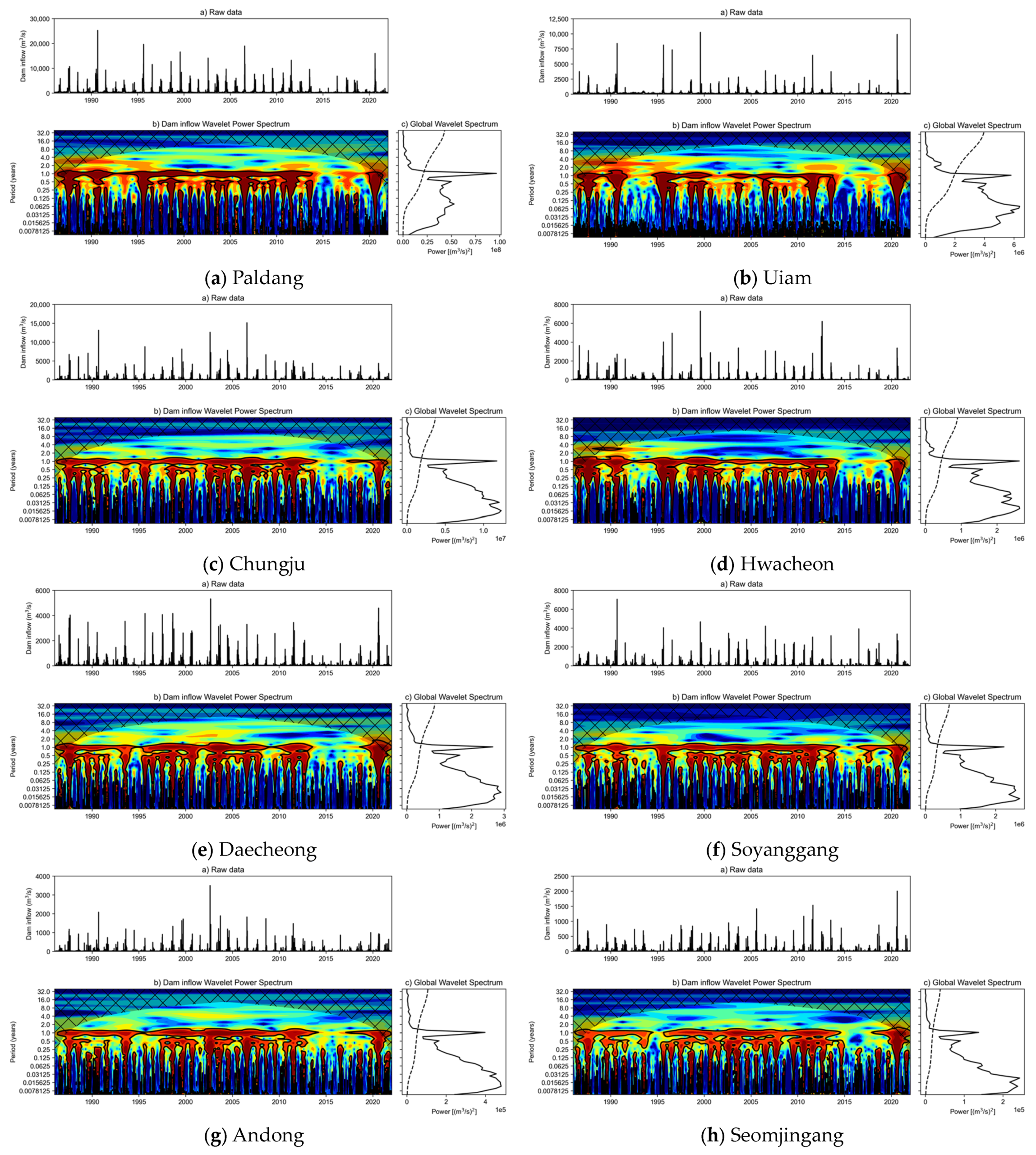
3.2. Wavelet Analysis

Figure 8 shows the results of wavelet analyses on the raw data. The annual cycle appears prominently. Although this trend is noted to be slightly weakened during the 2010s, the dams exhibit a more distinct annual cycle within one year except for the Paldang Dam. As the dam size decreases, a higher power is observed at a smaller scale. Except for the Paldang Dam and the Uiam Dam, the other dams exhibit very similar spectrum patterns. This appears to be influenced by the presence of hydraulic structures upstream. In other words, if there are structures such as dams upstream for flood management, the spectrum of shorter periods tends to be somewhat mitigated.
Notably, although the data exhibit significant annual periodicity, our focus is the variation in flow excluding seasonal fluctuations. Therefore, we performed a wavelet analysis after removing seasonality. Figure 9 presents the results of the same analysis conducted using data subjected to seasonal differencing. Unlike Figure 8, dam inflow in each figure in Figure 9 presents the seasonally differenced data. Based on seasonal differencing, data excluding the first year were used in the analysis.
Figure 9 shows that the annual periodic variations are eliminated, leaving only variations within the year. The variations within one year are not significant, and a smaller catchment corresponds to shorter period exhibiting the largest GWP. These trends are repeated almost every year. Therefore, similar results are likely to be obtained by the Fourier analysis. Considering these aspects, we extracted the period and corresponding frequency with the largest GWP.
Table 5 summarizes the period with the maximum GWP (M-GWP) and corresponding frequency. In ‘(c)’ in for each set of figures in Figure 9, the largest x-value represents the M-GWP, and its corresponding y-value indicates the period. The frequency is simply the reciprocal of the period. These results represent the strongest periodic component in a time series, excluding seasonal changes. For example, in the case of the Chungju Dam, the strongest component repeats every 0.032 y (approximately 11.7 d), occurring approximately 31.2 times in a year.

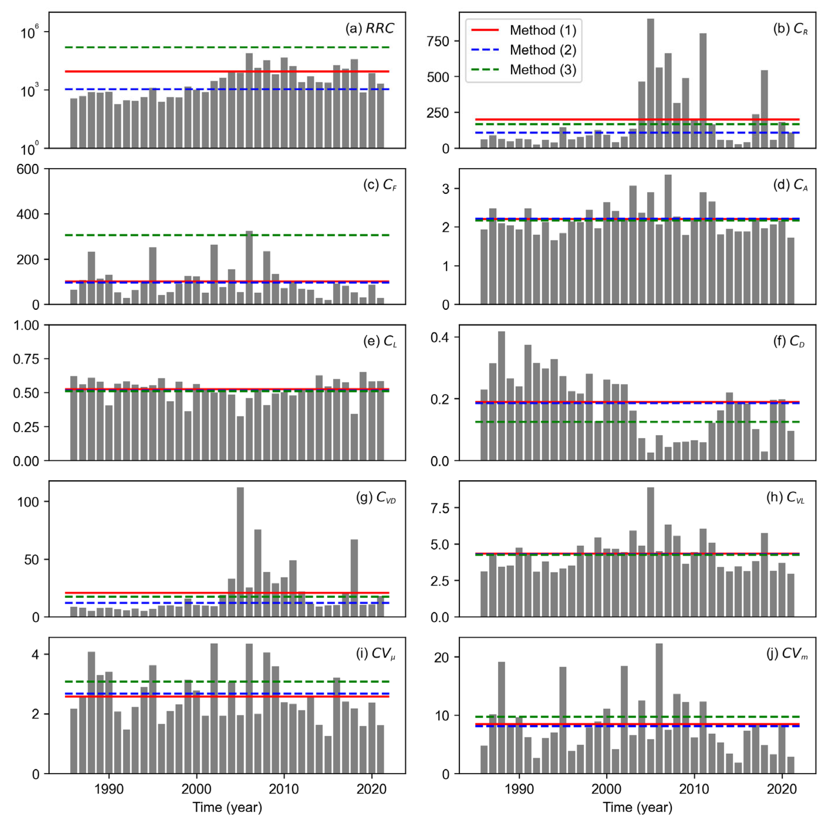
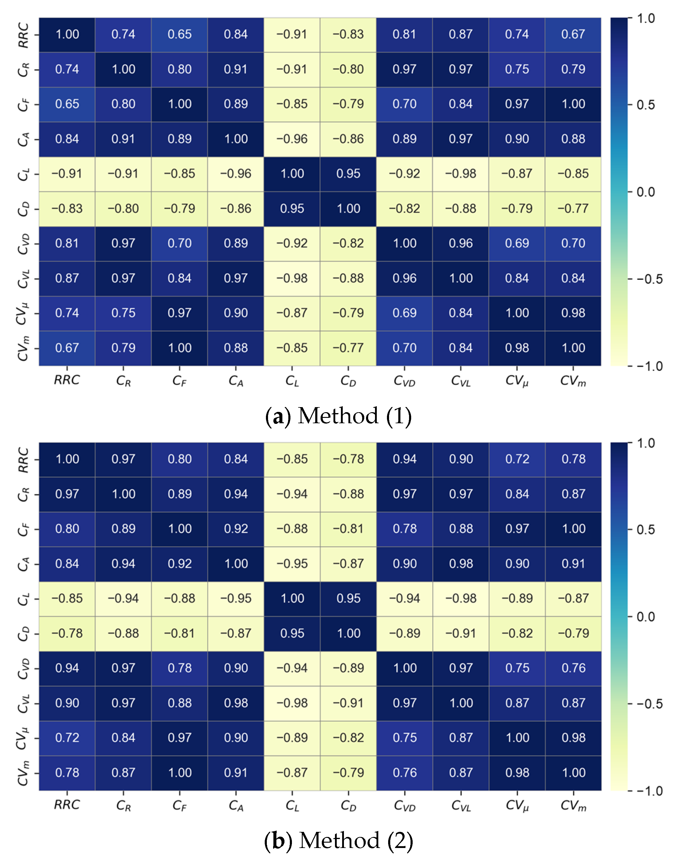
3.3. Evaluation of Methods for L-FFI Estimation

Figure 10 shows the results of analyzing the correlation among the L-FFIs. The trend is slightly different for the two groups ( C L and C D vs. the others). In other words, C L and C D are negatively correlated with the other indicators and positively correlated with each other. This observation suggests that in cases of strong high flow, low flow tends to weaken. The RRC exhibits the most notable differences depending on the method used. Only the RRC obtained using Method (2) exhibits a strong absolute correlation with the other indices.
The M-GWP frequency represents the frequency of non-seasonal flow repetitions. Thus, as this value increases, the likelihood of intensification of high and low flows compared with the average increases. Therefore, there exists a positive relationship with the high-flow index and negative relationship with the low-flow index, as shown in Figure 10.
Figure 11 displays the scatter plot of the M-GWP frequency and L-FFIs, and Figure 12 presents the corresponding correlation coefficient ( R ) and determination coefficient ( R 2 ). The M-GWP frequency is negatively correlated with C L and C D and positively correlated with the remaining indicators. Except for C L , the highest correlation is observed when the indicators are calculated using Method (2). When compared quantitatively using the coefficient of determination, for Method (1) the R 2   values range between 0.497 and 0.818, with an average R 2 of 0.686. On the other hand, Method (2) has a range of 0.548 to 0.829, with the highest average R 2 of 0.728. Lastly, Method (3) displays a range of 0.026 to 0.760, with an average R 2 of 0.559. The greatest difference can be observed in the RRC.

4. Discussion

In this study, we identified the strongest periodic components from the differenced data and data excluding seasonal variations, and selected the method that showed the most pronounced correlation with L-FFI. Overall, Method (2), which calculates the index by averaging the flow indices, emerges as the most reasonable approach. Method (2) can have the effect of smoothing outliers that may occur in each year, preserving information about long-term flow characteristics. This method can be used to calculate the L-FFI for any point on a dam or along a river, which can facilitate the establishment of appropriate strategies for water management.
Major related prior studies [6,7,8,9,10,11] vary in the periods they use for indicator estimation, and there are even instances within the same study where results from different periods are compared with one another. In contrast, the approach proposed in this study has a clear estimation method for each technique, and notably for Method (2)—which was evaluated as the most optimal—indicators sensitive to maximum values such as RRC appear within a much more acceptable range. Overall, when considering the representativeness of the basin, it is deemed more reasonable compared to previous studies.
We further analyzed the regionalization of watersheds. Ward’s method was utilized, one of the representative hierarchical clustering methods. In this study, we performed clustering using L-FFIs derived from Methods (1), (2), and (3) and also carried out clustering by utilizing GWP (global wavelet power) for comparison. Figure 13 displays the results. The standardization was conducted before the analysis.
Method (1) and Method (2) show almost similar analysis results, while Method (3) exhibits a somewhat different regionalization pattern. Observing the clustering results from the wavelet analysis, Method (3) closely aligns with the results of Method (2). This seems to support the findings of our earlier analysis. Moreover, in all analyses, we confirmed that the largest basins, Paldang and Uiam, are clustered differently. As mentioned in the wavelet analysis, this appears to be influenced by the presence of structures such as dams upstream for flood management.
The wavelet analysis employed in this study allows for the simultaneous capture of high-frequency and low-frequency components of time series, offering the advantage of investigating both short-term and long-term fluctuations. Moreover, it can be applied to non-stationary time series data, making it adept at capturing changes in extreme conditions such as droughts or floods. However, the interpretation of non-recurring single events can be somewhat challenging, and due to the inherent characteristics of wavelet analysis, the beginning and end of the time series may yield slightly distorted results. Therefore, caution is needed when interpreting data with shorter lengths. While this study conducted analyses on a daily scale, it is essential to note that for actual flood prevention, an even shorter time-scale analysis could be more critical.
Through the methodology of this study, if further analyses for multiple basins are conducted in the future, it will be possible to establish a range for long-term indicators that demonstrate hydrologically stable patterns. In such cases, any new basin can be evaluated through these long-term indicators, enabling the determination of whether improvements in hydrological cycles, through human interventions such as the installation of additional dams or river maintenance, are necessary. These series of processes are expected to facilitate long-term water resource management.
On the other hand, such variations in flow are derived from changes in precipitation patterns. Of course, the degree to which rainfall patterns manifest as changes in flow patterns will vary by basin. However, this study solely focused on determining the most rational method to quantify changes in flow. In future research endeavors, it is deemed essential to investigate the factors influencing long-term flow indicators, such as land cover, soil characteristics, and river network morphology. Furthermore, it is also necessary to examine how these factors respond to rainfall patterns. Additionally, a thorough examination of the implications of these indicators from the perspective of water resource management, specifically pertaining to water supply and flood prevention, is also warranted.

5. Conclusions

This study explored indices for quantifying flow fluctuations and calculated long-term flow indicators using different methods. For calculating L-FFIs, three approaches were considered. Wavelet analysis was performed to evaluate the derived L-FFI. The evaluation index focused on the period with the highest spectral power from the wavelet transformation of seasonally differenced daily dam inflow data. The key conclusions can be summarized as follows.
(1) The results varied greatly depending on the methodology used to determine the L-FFIs. The RRC, calculated as the ratio of the maximum and minimum flow values, was identified as the most sensitive index to the method used.
(2) Wavelet analysis of the data with seasonality removed revealed periodic components within a year exhibiting strong peaks. The period and frequency having maximum global wavelet powerderived from these data decreased and increased, respectively, with reduced dam size.
(3) The M-GWP frequency was positively and negatively correlated with the high-flow and low-flow indices, respectively. The strength of the correlations was the highest when using Method (2) with the highest average R 2 of 0.728.
(4) In the regionalization analysis using the Ward method, it was consistently observed that the Chungju Dam and Uiam Dam were significantly differentiated from the other dams. Furthermore, Method (2) showed the most similar characteristics to the clustering of the GWPs from the wavelet analysis.
Overall, Method (2), which involves averaging the flow indices to determine the L-FFI, was noted to be the most reasonable approach. In general, to facilitate efficient water management at the basin level and formulate effective policies, the flow must be analyzed considering various aspects. Indices representing high flow, such as the RRC , can be typically used to formulate flood control strategies, and indices representing low flow may be used to ensure effective water use. The strong correlation between the maximum frequency period and long-term FFIs is a key finding that can provide guidelines for basin management. If further analyses for multiple basins are conducted in the future, it will be possible to establish a range for long-term indicators that demonstrate hydrologically stable patterns. In such cases, the ungauged basin can be evaluated through these long-term indicators, helping in decision-making about human interventions in hydrological cycles. These processes are expected to facilitate long-term water resource management.

Author Contributions

Conceptualization, J.C.; data curation, G.M.; formal analysis, J.L. (Jiho Lee); investigation, C.J.; writing—original draft preparation, J.L. (Jinwook Lee); writing—review and editing, J.C. All authors have read and agreed to the published version of the manuscript.

Funding

This research was funded by the R&D Program for Forest Science Technology of Korea Forest Service (Korea Forestry Promotion Institute), grant number 2021365B10-2323-BD01.

Data Availability Statement

The data that support the findings of this study are available from the corresponding author upon reasonable request.

Conflicts of Interest

The authors declare no conflict of interest.

References

  1. Curry, R.A.; Gehrels, J.; Noakes, D.L.G.; Swainson, R. Effects of River Flow Fluctuations on Groundwater Discharge through Brook Trout, Salvelinus Fontinalis, Spawning and Incubation Habitats. Hydrobiologia 1994, 277, 121–134. [Google Scholar] [CrossRef]
  2. Huang, Y.; Schmitt, F.G.; Lu, Z.; Liu, Y. Analysis of Daily River Flow Fluctuations Using Empirical Mode Decomposition and Arbitrary Order Hilbert Spectral Analysis. J. Hydrol. 2009, 373, 103–111. [Google Scholar] [CrossRef]
  3. Hirpa, F.A.; Gebremichael, M.; Over, T.M. River Flow Fluctuation Analysis: Effect of Watershed Area. Water Resour. Res. 2010, 46, W12529. [Google Scholar] [CrossRef]
  4. Vesipa, R.; Camporeale, C.; Ridolfi, L. Effect of River Flow Fluctuations on Riparian Vegetation Dynamics: Processes and Models. Adv. Water Resour. 2017, 110, 29–50. [Google Scholar] [CrossRef]
  5. Chalise, D.R.; Sankarasubramanian, A.; Ruhi, A. Dams and Climate Interact to Alter River Flow Regimes across the United States. Earth Future 2021, 9, e2020EF001816. [Google Scholar] [CrossRef]
  6. Won, T.S. Discussing the Special Characteristics of Korean Rivers. KSCE J. Civ. Environ. Eng. Res. 1962, 10, 63–72. [Google Scholar]
  7. Park, S.W. A Hydrological Study on the Flow Characteristic of the Keum River. J. Korean Soc. Agric. Eng. 1974, 16, 3438–3453. [Google Scholar]
  8. Lee, J.W.; Woo, H.S. Analysis of River Regime of the Major Rivers in Korea. In Proceedings of the Korea Water Resources Association Conference, Daejeon, Republic of Korea, 10 July 1992; pp. 177–186. [Google Scholar]
  9. Lee, J.W.; Kim, H.S.; Woo, H.S. An Analysis of the Effect of Damming on Flow Duration Characteristics of Five Major Rivers in Korea. KSCE J. Civ. Environ. Eng. Res. 1993, 13, 79–91. [Google Scholar]
  10. Lee, E.H. A Study on the Change of the River-Regime Coefficient in the Han River and Nakdong River. Geogr. J. Korean 2008, 42, 211–222. [Google Scholar]
  11. Handayani, Y.L.; Sujatmoko, B.; Oktavia, G. Stream’s Regime Coefficient in Upstream Rokan Watershed of Riau Province. In MATEC Web of Conference, Proceedings of the International Conference on Advances in Civil and Environmental Engineering, Bali, Indonesia, 24–25 October 2018; EDP Sciences: Les Ulis, France, 2019; Volume 276, p. 04013. [Google Scholar]
  12. Cazelles, B.; Chavez, M.; Berteaux, D.; Ménard, F.; Vik, J.O.; Jenouvrier, S.; Stenseth, N.C. Wavelet Analysis of Ecological Time Series. Oecologia 2008, 156, 287–304. [Google Scholar] [CrossRef] [PubMed]
  13. Nakken, M. Wavelet Analysis of Rainfall–Runoff Variability Isolating Climatic from Anthropogenic Patterns. Environ. Modell. Softw. 1999, 14, 283–295. [Google Scholar] [CrossRef]
  14. Kailas, S.V.; Narasimha, R. Quasi-Cycles in Monsoon Rainfall by Wavelet Analysis. Curr. Sci. 2000, 78, 592–595. Available online: https://www.jstor.org/stable/24104088 (accessed on 1 May 2023).
  15. Souza Echer, M.P.; Echer, E.; Nordemann, D.J.; Rigozo, N.R.; Prestes, A. Wavelet Analysis of a Centennial (1895–1994) Southern Brazil Rainfall Series (Pelotas, 31 46′ 19″ S 52 20′ 33″ W). Clim. Chang. 2008, 87, 489–497. [Google Scholar] [CrossRef]
  16. Campozano, L.; Mendoza, D.; Mosquera, G.; Palacio-Baus, K.; Célleri, R.; Crespo, P. Wavelet Analyses of Neural Networks Based River Discharge Decomposition. Hydrol. Process. 2020, 34, 2302–2312. [Google Scholar] [CrossRef]
  17. Kumar, M.; Kumar, P.; Kumar, A.; Elbeltagi, A.; Kuriqi, A. Modeling Stage–Discharge–Sediment Using Support Vector Machine and Artificial Neural Network Coupled with Wavelet Transform. Appl. Water Sci. 2022, 12, 87. [Google Scholar] [CrossRef]
  18. Budu, K. Comparison of Wavelet-Based ANN and Regression Models for Reservoir Inflow Forecasting. J. Hydrol. Eng. 2014, 19, 1385–1400. [Google Scholar] [CrossRef]
  19. Kumar, S.; Tiwari, M.K.; Chatterjee, C.; Mishra, A. Reservoir Inflow Forecasting Using Ensemble Models Based on Neural Networks, Wavelet Analysis and Bootstrap Method. Water Resour. Manag. 2015, 29, 4863–4883. [Google Scholar] [CrossRef]
  20. Tran, T.D.; Tran, V.N.; Kim, J. Improving the Accuracy of Dam Inflow Predictions Using a Long Short-Term Memory Network Coupled with Wavelet Transform and Predictor Selection. Mathematics 2021, 9, 551. [Google Scholar] [CrossRef]
  21. Stefenon, S.F.; Seman, L.O.; Aquino, L.S.; Coelho, L. dos S. Wavelet-Seq2Seq-LSTM with Attention for Time Series Forecasting of Level of Dams in Hydroelectric Power Plants. Energy 2023, 274, 127350. [Google Scholar] [CrossRef]
  22. Labat, D. Wavelet Analysis of the Annual Discharge Records of the World’s Largest Rivers. Adv. Water Resour. 2008, 31, 109–117. [Google Scholar] [CrossRef]
  23. Ashraf, F.B.; Haghighi, A.T.; Riml, J.; Mathias Kondolf, G.; Kløve, B.; Marttila, H. A Method for Assessment of Sub-Daily Flow Alterations Using Wavelet Analysis for Regulated Rivers. Water Resour. Res. 2022, 58, e2021WR030421. [Google Scholar] [CrossRef]
  24. Yin, L.; Wang, L.; Keim, B.D.; Konsoer, K.; Zheng, W. Wavelet Analysis of Dam Injection and Discharge in Three Gorges Dam and Reservoir with Precipitation and River Discharge. Water 2022, 14, 567. [Google Scholar] [CrossRef]
  25. Ward, J.H. Hierarchical Grouping to Optimize an Objective Function. J. Am. Stat. Assoc. 1963, 58, 236–244. [Google Scholar] [CrossRef]
  26. Hartigan, J.A.; Wong, M.A. Algorithm AS 136: A K-Means Clustering Algorithm. J. R. Stat. Soc. C Appl. Stat. 1979, 28, 100–108. [Google Scholar] [CrossRef]
  27. Ouali, D.; Chebana, F.; Ouarda, T.B.M.J. Non-Linear Canonical Correlation Analysis in Regional Frequency Analysis. Stoch. Environ. Res. Risk Assess. 2016, 30, 449–462. [Google Scholar] [CrossRef]
  28. Ahani, A.; Mousavi Nadoushani, S.S.; Moridi, A. A Hybrid Regionalization Method Based on Canonical Correlation Analysis and Cluster Analysis: A Case Study in Northern Iran. Hydrol. Res. 2019, 50, 1076–1095. [Google Scholar] [CrossRef]
  29. Ahani, A.; Mousavi Nadoushani, S.S.; Moridi, A. Regionalization of Watersheds Based on the Concept of Rough Set. Nat. Hazards 2020, 104, 883–899. [Google Scholar] [CrossRef]
  30. Ahani, A.; Mousavi Nadoushani, S.S.; Moridi, A. Regionalization of Watersheds by Finite Mixture Models. J. Hydrol. 2020, 583, 124620. [Google Scholar] [CrossRef]
  31. Kanishka, G.; Eldho, T.I. Streamflow Estimation in Ungauged Basins Using Watershed Classification and Regionalization Techniques. J. Earth Syst. Sci. 2020, 129, 186. [Google Scholar] [CrossRef]
  32. Ferreira, R.G.; da Silva, D.D.; Elesbon, A.A.A.; dos Santos, G.R.; Veloso, G.V.; Fraga, M.d.S.; Fernandes-Filho, E.I. Geostatistical Modeling and Traditional Approaches for Streamflow Regionalization in a Brazilian Southeast Watershed. J. South Am. Earth Sci. 2021, 108, 103355. [Google Scholar] [CrossRef]
  33. Ahani, A.; Mousavi Nadoushani, S.S.; Moridi, A. A Ranking Method for Regionalization of Watersheds. J. Hydrol. 2022, 609, 127740. [Google Scholar] [CrossRef]
  34. Maidment, D.R. Handbook of Hydrology, 1st ed.; McGraw-Hill: New York, NY, USA, 1993. [Google Scholar]
  35. Park, S.D. Development and Management of Water Resources in South and North Gangwon-Do. In Understanding the Divided Gangwon-do: Situation and Prospects; Hanul Academy: Seoul, Republic of Korea, 1999; p. 605. [Google Scholar]
  36. Park, S.-D. Dimensionless Flow Duration Curve in Natural River. J. Korean Water Resour. Assoc. 2003, 36, 33–44. [Google Scholar] [CrossRef]
  37. Box, G.E.P.; Jenkins, G.M.; Reinsel, G.C. Autocorrelation Function and Spectrum of Stationary Processes and Analysis of Seasonal Time Series. In Time Series Analysis: Forecasting and Control, 2nd ed.; Holden-Day: San Francisco, CA, USA, 1976; pp. 21–43. [Google Scholar]
  38. Gardner, E.S., Jr. Exponential Smoothing: The State of the Art. J. Forecast. 1985, 4, 1–28. [Google Scholar] [CrossRef]
  39. Kalman, R.E. A New Approach to Linear Filtering and Prediction Problems. J. Basic Eng. 1960, 82, 35–45. [Google Scholar] [CrossRef]
  40. Rabiner, L.R. A Tutorial on Hidden Markov Models and Selected Applications in Speech Recognition. Proc. IEEE 1989, 77, 257–286. [Google Scholar] [CrossRef]
  41. Sims, C.A. Macroeconomics and Reality. Econometrica 1980, 48, 1–48. [Google Scholar] [CrossRef]
  42. Huang, N.E.; Long, S.R.; Shen, Z. The Mechanism for Frequency Downshift in Nonlinear Wave Evolution. In Advances in Applied Mechanics; Hutchinson, J.W., Wu, T.Y., Eds.; Elsevier: Amsterdam, The Netherlands, 1996; Volume 32, pp. 59–117C. [Google Scholar]
  43. Rehman, N.; Mandic, D.P. Multivariate Empirical Mode Decomposition. Proc. R. Soc. A Math. Phys. Eng. Sci. 2009, 466, 1291–1302. [Google Scholar] [CrossRef]
  44. Duan, J.-S.; Rach, R. A New Modification of the Adomian Decomposition Method for Solving Boundary Value Problems for Higher Order Nonlinear Differential Equations. Appl. Math. Comput. 2011, 218, 4090–4118. [Google Scholar] [CrossRef]
  45. Turkyilmazoglu, M. Accelerating the Convergence of Adomian Decomposition Method (ADM). J. Comput. Sci. 2019, 31, 54–59. [Google Scholar] [CrossRef]
  46. Cohen, L. Time-Frequency Analysis. In Prentice Hall Signal Processing, 1st ed.; Prentice Hall: Englewood Cliffs, NJ, USA, 1995; Volume 778. [Google Scholar]
  47. Hlawatsch, F.; Auger, F. Time-Frequency Analysis: Concepts and Methods; John Wiley & Sons: Hoboken, NJ, USA, 2008. [Google Scholar]
  48. Wigner, E.P. On the Quantum Correction for Thermodynamic Equilibrium. In Part I: Physical Chemistry. Part II: Solid State Physics; Springer: Heidelberg, Germany, 1997; pp. 110–120. [Google Scholar]
  49. Smith, L.C.; Turcotte, D.L.; Isacks, B.L. Stream Flow Characterization and Feature Detection Using a Discrete Wavelet Transform. Hydrol. Process. 1998, 12, 233–249. [Google Scholar] [CrossRef]
  50. Gabor, D. Theory of Communication. Part 1: The Analysis of Information. J. Inst. Electr. Eng. Part III Radio Commun. Eng. 1946, 93, 429–441. [Google Scholar] [CrossRef]
  51. Misiti, M.; Misiti, Y.; Oppenheim, G.; Poggi, J.-M. Wavelets and Their Applications, 1st ed.; ISTE: London, UK, 2007; ISBN 978-1-905209-31-6. [Google Scholar]
  52. Ngui, W.K.; Leong, M.S.; Hee, L.M.; Abdelrhman, A.M. Wavelet Analysis: Mother Wavelet Selection Methods. Appl. Mech. Mater. 2013, 393, 953–958. [Google Scholar] [CrossRef]
  53. Aguiar-Conraria, L.; Azevedo, N.; Soares, M.J. Using Wavelets to Decompose the Time–Frequency Effects of Monetary Policy. Physica A 2008, 387, 2863–2878. [Google Scholar] [CrossRef]
  54. Rua, A. Measuring Comovement in the Time–Frequency Space. J. Macroecon. 2010, 32, 685–691. [Google Scholar] [CrossRef]
  55. Lee, J.; Lee, H.; Yoo, C. Selection of mother wavelet for bivariate wavelet analysis. J. Korean Water Resour. Assoc. 2019, 52, 905–916. [Google Scholar] [CrossRef]
  56. Grinsted, A.; Moore, J.C.; Jevrejeva, S. Application of the Cross Wavelet Transform and Wavelet Coherence to Geophysical Time Series. Nonlinear Process. Geophys. 2004, 11, 561–566. [Google Scholar] [CrossRef]
  57. Torrence, C.; Compo, G.P. A Practical Guide to Wavelet Analysis. Bull. Amer. Meteorol. Soc. 1998, 79, 61–78. [Google Scholar] [CrossRef]
  58. Srinivas, V.V. Regionalization of Watersheds Using Soft Computing Techniques. ISH J. Hydraul. Eng. 2009, 15, 170–193. [Google Scholar] [CrossRef]
  59. Yang, T.; Shao, Q.; Hao, Z.-C.; Chen, X.; Zhang, Z.; Xu, C.-Y.; Sun, L. Regional Frequency Analysis and Spatio-Temporal Pattern Characterization of Rainfall Extremes in the Pearl River Basin, China. J. Hydrol. 2010, 380, 386–405. [Google Scholar] [CrossRef]
  60. Hassan, B.G.; Ping, F. Formation of Homogenous Regions for Luanhe Basin-by Using L-Moments and Cluster Techniques. Int. J. Environ. Sci. Dev. 2012, 3, 205. [Google Scholar] [CrossRef]
  61. Sharghi, E.; Nourani, V.; Soleimani, S.; Sadikoglu, F. Application of Different Clustering Approaches to Hydroclimatological Catchment Regionalization in Mountainous Regions, a Case Study in Utah State. J. Mt. Sci. 2018, 15, 461–484. [Google Scholar] [CrossRef]
  62. Ramachandra Rao, A.; Srinivas, V.V. Regionalization of Watersheds by Hybrid-Cluster Analysis. J. Hydrol. 2006, 318, 37–56. [Google Scholar] [CrossRef]
  63. Hosking, J.R.M.; Wallis, J.R. Regional Frequency Analysis; Cambridge University Press: Cambridge, UK, 1997. [Google Scholar]
Figure 1. Location of eight dam basins considered in this study.
Water 15 02968 g001
Figure 2. Daily inflow (black solid line) and mass curve (blue dashed line) of Chungju Dam from 1986 to 2021.
Water 15 02968 g002
Figure 3. Daily precipitation (black solid line) and mass curve (blue dashed line) of Chungju Dam from 1986 to 2021.
Water 15 02968 g003
Figure 4. Annual variations in the flow characteristics of the Chungju Dam basin.
Water 15 02968 g004
Figure 5. Box−plots for annual flows on log scale of the Chungju Dam basin.
Water 15 02968 g005
Figure 6. FFIs and L-FFIs for the Chungju Dam basin by year, determined using different methods.
Water 15 02968 g006
Figure 7. L-FFIs of all dam basins, determined using different methods.
Water 15 02968 g007
Figure 8. Wavelet analysis results using raw data. For each set of figures, (a) denotes the data for wavelet analysis, (b) represents the results of the wavelet analysis, and (c) indicates the global power of the wavelet. The dark solid line in (b) and dotted line in (c) indicate the 95% confidence level.
Water 15 02968 g008
Figure 9. Wavelet analysis results using seasonally differenced data. For each set of figures, (ac) are the same as described in Figure 8.
Water 15 02968 g009
Figure 10. Heatmaps of correlation coefficients among the LFFIs determined using different methods. Method (1): calculate the annual index and then average it; Method (2): average the annual flow characteristics and then calculate the index; and Method (3): calculate the index considering all available data.
Water 15 02968 g010aWater 15 02968 g010b
Figure 11. Scatter plots of the M-GWP frequency vs. L-FFIs. In (a), the red box zooms in on the red shadow region (RRC of 0–10,000).
Water 15 02968 g011
Figure 12. Heatmap of (a) correlation coefficient and (b) determination coefficient among the M-GWP frequency vs. L-FFIs obtained using different methods.
Water 15 02968 g012
Figure 13. Results of regionalization through cluster analysis. (ac) utilized all L-FFIs considered in this study, while (d) employed the global wavelet power for all scales.
Water 15 02968 g013
Table 1. Basic information on dam basins.
Dam NameBasin Area (km2)Channel Length (km)Total Storage (106 m3)
Paldang23,800377.6244
Uiam7709230.980
Chungju6648270.62750
Hwacheon3901178.11018
Daecheong3204208.11490
Soyanggang2703136.02900
Andong1584142.41248
Seomjingang76374.2466
Table 2. Flow fluctuation index (FFI) and description.
SymbolEquationIndexDescription
R R C Q max / Q min River regime coefficientThe ratio of the maximum flow to the minimum flow
C R Q 2.7 / Q 97.3 Flow regime coefficientThe ratio of the high flow to the low flow excepting for the extreme flows
C F Q m a x / Q 50.7 Flood coefficientThe ratio of the maximum flow to the approximate mode flow
C A Q 26.0 / Q 50.7 Abundance coefficientThe ratio of the approximate third quartile flow to the approximate median flow
C L Q 75.3 / Q 50.7 Low coefficientThe ratio of the approximate first quartile flow to the approximate median flow
C D Q 97.3 / Q 50.7 Drought coefficientThe ratio of the high flow to the approximate median flow
C V D Q 26.0 / Q 97.3 Variance of the drought coefficientThe ratio of the approximate third quartile flow to the low flow
C V L Q 26.0 / Q 75.3 Variance of the low
coefficient
The ratio of the approximate third quartile flow to the approximate first quartile flow
C V μ Q σ / Q μ Coefficient of variance based on meanThe variation of the flows to the mean flow
C V m Q σ / Q m Coefficient of variance based on medianThe variation of the flows to the median flow
Table 3. Yearly minimum and maximum flows and their derived RRCs for the Chungju Dam.
YearMinMaxRRCYearMinMaxRRC
198610.33683.9357.720044.14154.61013.3
198714.46731.8467.520052.11586.5755.5
19888.16121.9755.820064.412,599.52863.5
198910.07043.6704.420071.35575.24288.6
199017.013,142.1773.120081.07808.17808.1
199112.92427.0188.120090.43084.27710.5
19926.01692.0282.020100.215,126.475,632.0
199316.04250.0265.620110.22735.213,676.0
19949.64003.4417.020120.26662.333,311.5
19957.18776.21236.120130.85012.76265.9
19966.11496.3245.320140.14586.145,861.0
19978.03428.5428.620150.35059.916,866.3
199814.85897.2398.520161.43373.72409.8
19995.58156.71483.020170.94379.94866.6
20004.14154.61013.320180.4989.12472.8
20012.11586.5755.520190.3700.42334.7
20024.412,599.52863.520200.23663.718,318.5
20031.35575.24288.620210.22467.112,335.5
Table 4. L-FFIs of Chungju Dam basin, determined using different methods.
IndexMethod (1)Method (2)Method (3)
R R C 8723.51059.8151,264.0
C R 200.4108.1167.7
C F 100.996.2305.6
C A 2.22.22.2
C L 0.50.50.5
C D 0.20.20.1
C V D 20.712.017.3
C V L 4.34.34.3
C V μ 2.62.73.1
C V m 8.48.19.7
Table 5. Maximum global wavelet power and corresponding period and frequency.
DamM-GWP [(m3/s)2]Period (year)Frequency (1/y)
Paldang107,505,8640.07613.1
Uiam13,904,1770.04522.1
Chungju25,609,2690.03231.2
Hwacheon5,821,6730.04522.1
Daecheong6,286,0090.03826.3
Soyanggang5,658,0150.02737.1
Andong979,6270.02344.2
Seomjingang488,9830.02344.2
Disclaimer/Publisher’s Note: The statements, opinions and data contained in all publications are solely those of the individual author(s) and contributor(s) and not of MDPI and/or the editor(s). MDPI and/or the editor(s) disclaim responsibility for any injury to people or property resulting from any ideas, methods, instructions or products referred to in the content.

