Evaluating Underwater Light Availability for Phytoplankton: Mean Light Intensity in the Mixed Layer versus Attenuation Coefficient

Abstract

The use of several light-related variables, such as the Secchi disc depth, the euphotic depth, and in particular, the diffuse attenuation coefficient (K_d), is deeply rooted in phytoplankton research, but these are not the most appropriate indicators of the amount of light available for photosynthesis. We argue that the variable of interest for phytoplankton is the mean light intensity in the mixed layer (I_m), which represents the mean light to which phytoplankton cells are exposed throughout their life cycle, while being continuously mixed in the mixed layer. We use empirical data collected in different coastal ecosystems in southern Portugal to demonstrate why I_m should be the preferred metric instead of the deeply rooted K_d. We show that, although the relationship between I_m and K_d is inversely proportional, it is not always strong or even significant. Different I_m values can be associated with the same K_d, but distinct I_m have different physiological effects of phytoplankton. Therefore, K_d does not capture the amount of light available for photosynthesis, given that, unlike I_m, K_d calculation does not consider the depth of the mixed layer. Therefore, we urge phytoplankton researchers to consider the measurement and calculation of I_m when evaluating light-related processes in phytoplankton ecology.

1. Introduction

Light availability is of paramount importance for phytoplankton, especially in turbid ecosystems [1,2,3,4,5], but it has not yet received the same attention as nutrients as an environmental driver of phytoplankton dynamics. For instance, studies evaluating the effects of nutrient enrichment using phytoplankton microcosms or mesocosms are abundant (e.g., [6,7]), whilst experiments testing the effects of light on phytoplankton growth, production, or composition are rather scarce (e.g., [8,9]). The main reason behind this discrepancy is probably methodological. Dissolved inorganic macronutrients can be easily and directly analyzed in the lab, using simple colorimetric methods (e.g., [10]). In addition, water samples can be collected and preserved for a considerable amount of time before the actual nutrient analysis is performed.

Measurements of underwater light are not as straightforward. Solar radiation reaching the Earth’s surface is composed of a large spectrum of radiation with different energies and wavelengths, including ultraviolet, infrared, and visible radiation. Photoautotrophic organisms, such as plants and algae, can only use a fraction of the total solar radiation for the process of photosynthesis; this photosynthetically active radiation (PAR) corresponds roughly to the visible light of the electromagnetic spectrum, with wavelengths between 400 and 700 nm. PAR constitutes approximately 45% of the total solar radiation that reaches the Earth’s surface (when the solar elevation is more than 30°), considering both direct and diffuse sources [11]. The amount of light that penetrates the water surface depends on several factors, such as solar elevation and its daily and annual variation [12], but a reflectance of 6.6% for a flat water surface and irradiance coming equally from all directions is generally assumed [11]. The radiation that penetrates the water is scattered and eventually photons are absorbed by water molecules and by dissolved and particulate matter, resulting in an exponential decrease in light intensity with depth, according to the Beer–Lambert law. The rate at which light disappears in the water column with depth can be expressed by the light extinction coefficient or diffuse attenuation coefficient (K_d). K_d is classified as an apparent optical property of water, depending on the composition of the medium and on the directional structure of the ambient light field [11].

The diffuse attenuation coefficient is typically estimated using the depth of disappearance of the Secchi disc (SD) as k/SD, where k is a constant; k values of 1.7 [13] and 1.44 [14], for non-turbid (euphotic depth > 5 m) and turbid (euphotic depth < 5 m) waters, respectively, are commonly used. However, the constant k can vary widely, between 1.27 and 2 [15], and this uncertainty may lead to errors in the estimation of light availability for phytoplankton. In addition, this equation does not account for all of K_d variability, which is affected by any optically active component and represents the sum of water, phytoplankton, seston, and chromophoric dissolved organic matter (CDOM) variability [16]. Indeed, the relationship between SD and K_d may vary seven-fold in waters with high turbidity and CDOM variability [17].

The best estimate of K_d (m⁻¹) is given by an exponential fit of light measurements in the water column as a function of depth, according to Equation (1), based on the Beer–Lambert law:

$${\mathrm{I}}_{\mathrm{Z}}={\mathrm{I}}_0{\mathrm{e}}^{(-{\mathrm{K}}_{\mathrm{d}}\mathrm{Z})}$$

(1)

where I_Z (µmol photons m⁻² s⁻¹) is the light intensity at depth level Z (m) and I₀ is the light intensity at the water surface. Instead of the exponential fitting, K_d can be more accurately estimated with a linear fitting of log-transformed light values [18] (Equation (2)):

$${\mathrm{K}}_{\mathrm{d}}=\ln \left(\frac{{\mathrm{I}}_1}{{\mathrm{I}}_2}\right)/({\mathrm{Z}}_2-{\mathrm{Z}}_1)$$

(2)

where I₁ and I₂ are the light intensities at depth levels Z₁ and Z₂, respectively. Z₁ is the depth immediately below the water surface. When light intensity in the water column is not available, K_d is generally estimated using empirical coefficients. Yet, a hyperbolic fit of Secchi disk measurements and K_d (obtained from vertical light attenuation measurements) data will result in a better function to estimate K_d from SD in a given ecosystem, than these constants (e.g., [16]).

The use of the light attenuation coefficient is deeply rooted in phytoplankton research and many efforts have been made to develop better empirical relationships between the Secchi depth and K_d (e.g., [19,20,21]). However, the diffuse attenuation coefficient per se does not provide any information on the quantity of photosynthetically active radiation available for phytoplankton and, therefore, does not allow the evaluation of the underwater light environment and its role as a limiting factor of phytoplankton growth. To determine the potential light limitation, light intensity values are needed, just like nutrient concentrations are required to assess nutrient limitation [22,23]. Thus, the mean light intensity in the mixed layer (I_m) is a more relevant metric to evaluate the underwater light environment.

The mean light intensity in the mixed layer represents the mean photosynthetically active radiation to which cells are exposed throughout most of their life cycle, while being continuously mixed in the mixed layer. I_m is therefore a useful indicator of the underwater light environment, and it can be used to evaluate the occurrence of potential light limitation of phytoplankton growth. I_m determination (Equation (3)) considers the incident light at the water surface (I₀), the diffuse attenuation coefficient in the water column (K_d), and the depth of the mixed layer (Z_m):

$${\mathrm{I}}_{\mathrm{m}}={\mathrm{I}}_0(1-{\mathrm{e}}^{(-{\mathrm{K}}_{\mathrm{d}}\mathrm{Z})}){({\mathrm{K}}_{\mathrm{d}}{\mathrm{Z}}_{\mathrm{m}})}^{-1}$$

(3)

However, given the easiness of Secchi depth determination, the high cost of quanta sensors [20], and the common lack of daily integrated I₀ measurements, necessary for a realistic determination of I_m, K_d is frequently the only light-related variable determined in phytoplankton studies. In our opinion, K_d is used in a rather excessive and forced fashion to draw askew conclusions about the amount of light available for phytoplankton photosynthesis. It is commonly assumed that the relationship between K_d and light availability is inversely proportional, but light availability for phototrophs depends on the depth of the mixed layer, whereas K_d is unrelated with depth. For instance, a turbid (higher K_d) and shallow ecosystem (e.g., a coastal lagoon) may present higher light availability than a non-turbid system (lower K_d) with a deeper mixing layer (e.g., coastal zone, continental shelf, oceanic zone).

The assessment of underwater light availability is essential to understand phytoplankton dynamics and thus to assess the impacts of natural and human-induced perturbations to ecosystems. In this article, we aim to expose constraints that phytoplankton researchers are faced with when characterizing the underwater light environment and to clarify the light-related variables of interest that, in our opinion, should be used in phytoplankton research and environmental monitoring. To accomplish this goal, we present underwater light data collected in distinct ecosystems in southern Portugal and analyze relationships between the diffuse attenuation coefficient and mean light intensity in the mixed layer.

2. Materials and Methods

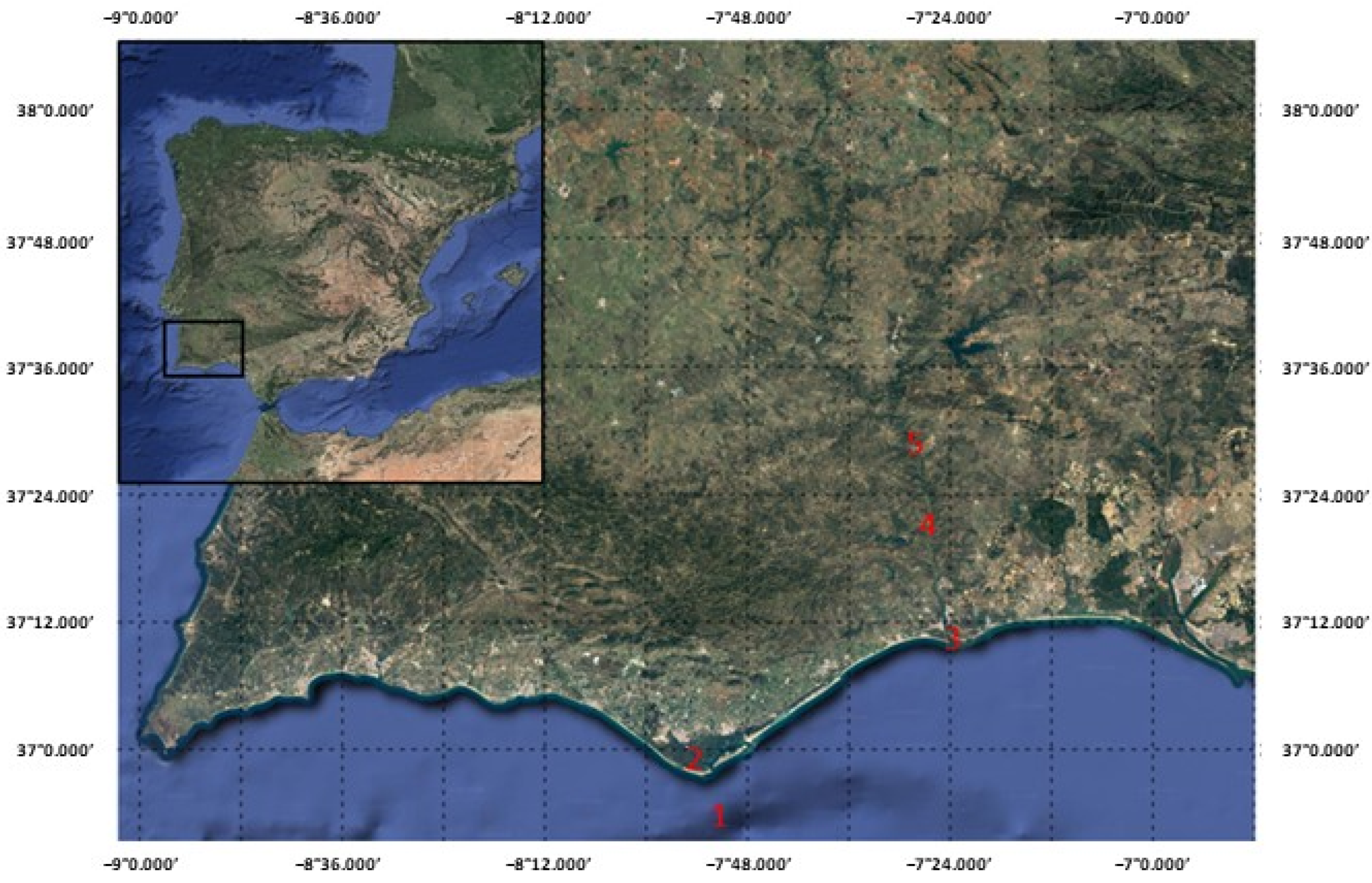
Several light variables were measured in three distinct ecosystems in southern Portugal (SW Iberia): the Guadiana estuary (divided into freshwater, brackish, and marine zones), the Ria Formosa coastal lagoon, and the coastal zone adjacent to the Ria Formosa coastal lagoon (Figure 1). Measurements were integrated in different research projects aimed at phytoplankton dynamics and results were published elsewhere [5,24,25]. Data presented here were collected from 2001 to 2009 in the Guadiana estuary, and between 2012 and 2014 in the Ria Formosa coastal lagoon and adjacent coastal zone.

Light penetration in the water column was determined using two methods: (a) calculation of K_d based on the disappearance of the Secchi disc and (b) calculation of I_m based on vertical profiles of PAR intensity. Using the disappearance of the Secchi disc, i.e., the Secchi depth (SD), the diffuse attenuation coefficient (k_d, m⁻¹) was calculated as 1.4/SD for highly turbid ecosystems [14], namely the Guadiana estuary, or as 1.7/SD for non-turbid ecosystems [13], namely the Ria Formosa coastal lagoon and the adjacent coastal zone; the use of these constants was based on the calculation of the euphotic depth, as 2.8 SD, which corresponds to the depth where light is 1% of incident light at the surface.

For the vertical profiles of PAR intensity in the mixed layer (I_m, µmol photons m⁻² s⁻¹), light intensity was measured every meter using a LI-COR 4π quantum sensor and K_d was calculated according to Equation (1) (see Section 1). The mean light intensity in the mixed layer (I_m, µmol photons m⁻² s⁻¹) was calculated according to Equation (3) [26]. The depth of the mixed layer, necessary for I_m calculation, was based on vertical profiles of temperature and salinity for the Ria Formosa and the Guadiana estuary (see Section 3); for the adjacent coastal zone, Z_m values were taken from [25]. Z_m values used for each station were 2 m for the Ria Formosa coastal lagoon; between 5.9 m and 9.9 m for the Guadiana estuary, depending on the location; and between 19.2 and 60.7 for the adjacent coastal zone, depending on the season.

Data analysis was carried out by means of descriptive statistics; Pearson’s correlation was conducted to assess the relationships between the mean light intensity in the mixed layer and the light attenuation coefficient. All data analyses were performed using IBM SPSS Statistics 28.

3. Results and Discussion

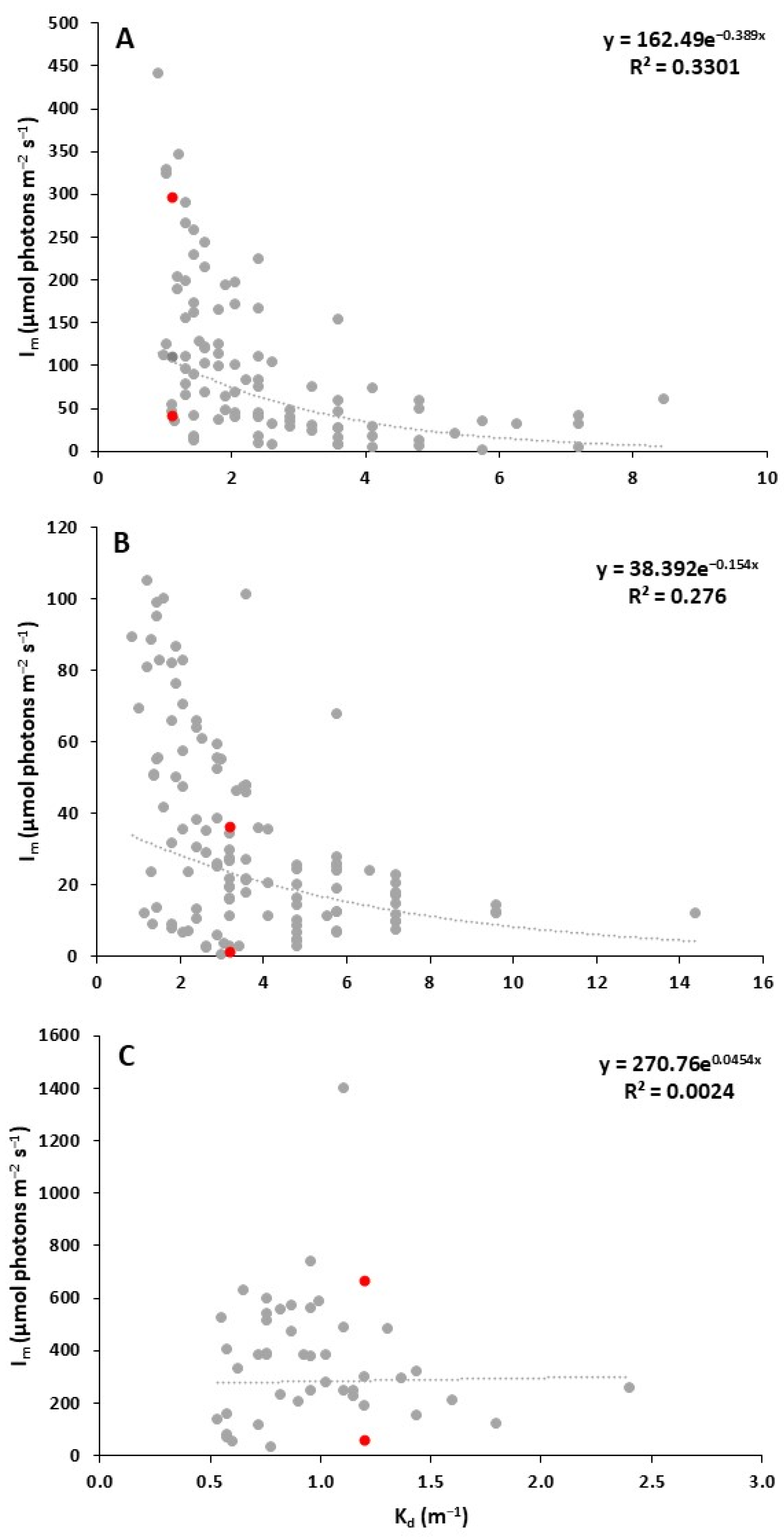
The relationship between the diffuse attenuation coefficient and the amount of light available for photosynthesis, expressed as the mean light intensity in the mixed layer, is typically inversely proportional, but not always significant. 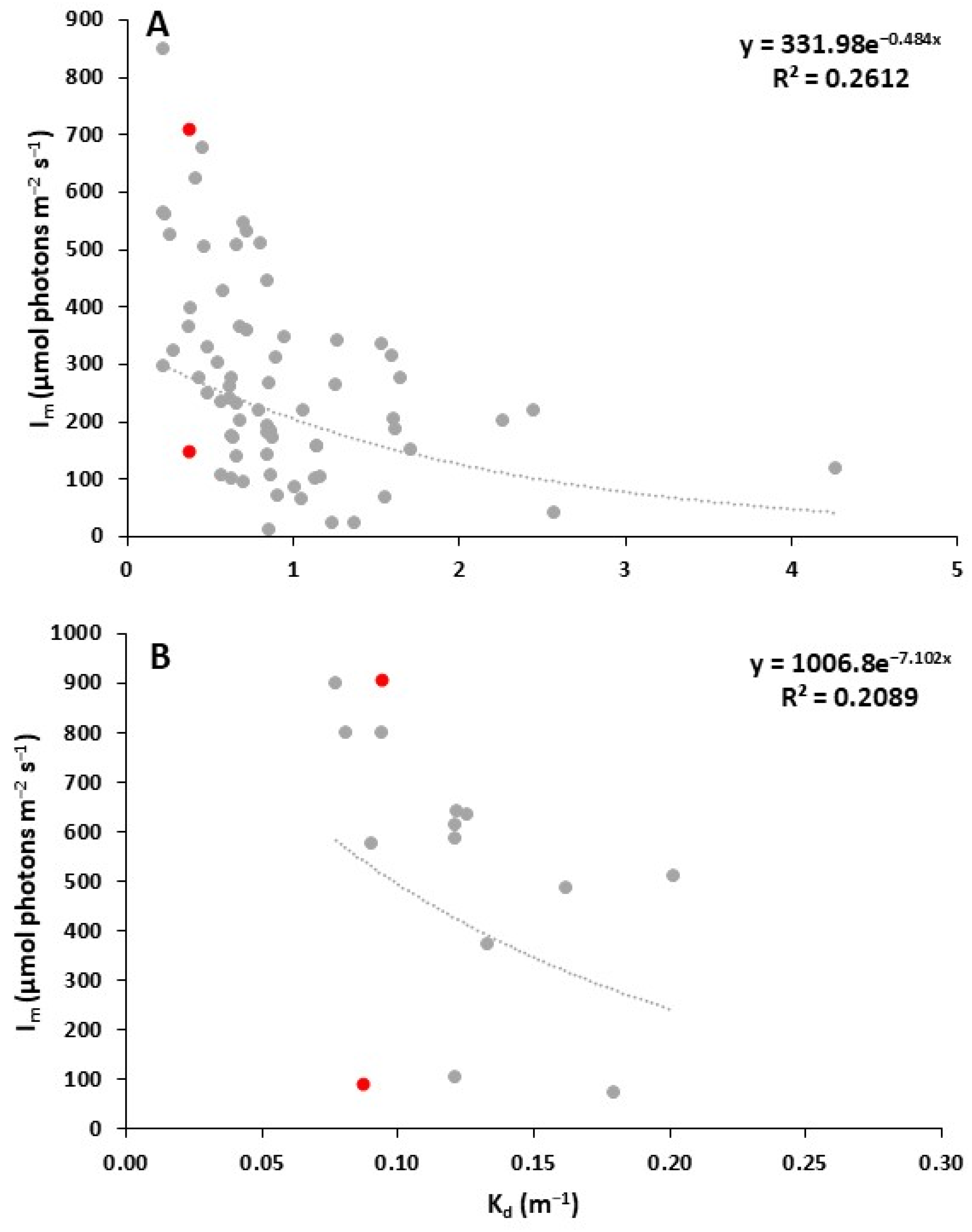The highest K_d and lower I_m values were found in the freshwater (K_d = 0.90–8.47 m⁻¹, I_m = 0.99–440.86 µmol photons m⁻² s⁻¹) and brackish (K_d = 0.85–14.40 m⁻¹; I_m = 0.42–104.97 µmol photons m⁻² s⁻¹) estuarine zones of the Guadiana estuary (Figure 2), whereas for coastal locations, K_d values were lower and I_m was higher (K_d = 0.08–4.26 m⁻¹, I_m = 12.82–1397.64 µmol photons m⁻² s⁻¹) (Figure 3). The strength of the relationship between the two variables in the different coastal ecosystems was always weak, with correlation coefficients ranging between 0.00 and 0.33.

It was also clear that similar light attenuation coefficients were associated with different mean light intensities (

Table 1. Examples of K_d (m⁻¹, obtained using Secchi disc depth) and corresponding I_m values (µmol photons m⁻² s⁻¹) for different types of ecosystems. The ten K_d × I_m values are represented as red dots in Figure 2 and Figure 3.

Ecosystem	Kd	Associated Im Values
Estuary–freshwater	1.1	42, 30
Estuary–brackish	3.2	1, 36
Estuary–marine	1.2	56, 67
Coastal lagoon	0.4	146, 71
Adjacent coastal waters	0.1	89, 91

), reflecting the importance of considering the depth of the mixed layer to properly evaluate PAR availability for photosynthesis and growth. For instance, a K_d of 0.6 m⁻¹ corresponds to I_m values ranging between 100 and 427 µmol photons m⁻² s⁻¹ in the Ria Formosa coastal lagoon, and between 50 and 332 µmol photons m⁻² s⁻¹ in the Guadiana estuary (see Figure 2 and Figure 3). For each type of ecosystem, the same K_d value was associated with a wide range of corresponding I_m values; for instance, in the coastal zone, a K_d of 0.09 m⁻¹ was associated with I_m values of 89 and 907 µmol photons m⁻² s⁻¹ (Table 1). These distinct I_m values may have different physiological effects on phytoplankton dynamics. For instance, light enrichment experiments conducted in the Guadiana estuary demonstrated that exposure of natural phytoplankton communities to I_m values of 50, 70, 120, and 225 µmol photons m⁻² s⁻¹ had significantly different effects, from an enhancement of phytoplankton growth to a decline in phytoplankton growth, consequently leading to changes in phytoplankton biomass and community structure [4]. Therefore, a K_d value of 0.6 m⁻¹ may correspond not only to different mean light intensities in the mixed layer, but also to different degrees of light limitation, light-limited growth, and photoinhibition of phytoplankton photosynthesis. To avoid erroneous conclusions about the availability of underwater light for phytoplankton based solely on light attenuation coefficients, we urge phytoplankton researchers to include estimates of both K_d and I_m in phytoplankton studies and monitoring programs. But how can the mean light intensity in the mixed layer be estimated in a timely and inexpensive manner?

First, the depth of the mixed layer (Z_m) should be established. The mixed layer is the top, unstratified layer in the water column where no significant density gradients are found, and phytoplankton is thus continuously mixed. Empirically, the mixed layer is usually an isothermal layer, where there is little variation in temperature with depth [27]; different thresholds to define Z_m have been used (e.g., [28]), but <0.5 °C is the most common in ocean and coastal waters [29]. In shallow, well-mixed ecosystems, Z_m usually corresponds to the whole water column depth [30]. In an estuarine ecosystem, for instance, Z_m will vary along the channel’s cross-section and with tidal phase. A mean mixing depth should therefore be established for coastal, shallow waters, taking into consideration bathymetry and tidal amplitude, which affect the depth of the water column. For deeper waters, the mixing depth should be determined in each sampling campaign, using vertical profiles of temperature and salinity.

A common lapse in phytoplankton studies is the characterization of light availability for phytoplankton using, besides the light attenuation coefficient, the compensation depth that corresponds to the bottom of the euphotic zone and is defined as the depth where the intensity of photosynthetically active radiation is 1% of incident PAR. Given that this amount of PAR is sufficient to sustain photosynthesis, the compensation depth is another metric widely used in phytoplankton research (e.g., [31]). However, the euphotic layer and the mixed layer are usually neither coincident nor proportional, and whilst the euphotic depth depends on inherent optical properties of the water, the mixing depth is mainly affected by physical-meteorological forcing, bathymetry, and even tides. For phytoplankton, it really does not matter how deep the euphotic zone is; what matters is the mean light intensity to which cells are exposed while being continuously mixed in the mixed layer. A useful approach, given by [32], combines both the euphotic depth and the mixing depth to characterize light availability for phytoplankton growth in the form of a mixing depth to euphotic depth ratio (Z_m:Z_eu). It is usually considered that when the mixing depth is more than five times the euphotic depth (Z_m:Z_eu > 5), net phytoplankton growth will not be possible.

Second, the light attenuation coefficient must be determined to calculate I_m. Two methods can be used, as referred above: vertical profiles of PAR in the water column or a function that relates light attenuation with Secchi depth. PAR measurements with a spherical quantum sensor are more reliable than the Secchi disk, which depends on the sensitivity of the human eye. But even vertical profiles of PAR are not exempt from problems. Several measurements of PAR intensity should be taken in the water column at specified depths (usually every meter), to adjust the exponential function based on the Beer–Lambert law. All measurements must be made in the same conditions, considering intermittent cloud cover and making sure that the cable supporting the light sensor is always vertical. Light attenuation is usually considered constant with depth, so only a few data points are necessary for an accurate estimate of K_d, especially in turbid systems, where light attenuation closely follows an exponential function and thus can be characterized by a single K_d [11]. In clear waters, the light attenuation with depth may present a biphasic behavior, characterized by two K_d values [11]. Another, more reliable method of obtaining vertical profiles of PAR intensity can be used. Instead of using just one light sensor, the two-bulb sensor method can be used. This method is based on light measurements by two light sensors mounted at a fixed vertical distance, allowing for simultaneous measurements of PAR intensity at two different depths [33]. The two-sensor method represents an improvement relative to the single sensor, as it provides profiles and instant PAR measurements at two depths, rather than isolated and non-concomitant PAR measurements [33].

It should be noted, however, that light attenuation in the water column may show significant daily variability. In shallow turbid ecosystems, significant and positive correlations between suspended particulate matter (SPM) and light attenuation are common, indicating that the attenuation of light is mainly controlled by suspended sediments [34,35], which in turn may show significant short-term variability associated with tidal cycles and river flow [2]. For instance, SPM in the Guadiana estuary is usually higher during spring tides, due to stronger tidal currents and higher resuspension of bottom sediments [35], and during flood, due to the resuspension of sediments deposited during the preceding long low-tide slack [36]. However, light attenuation coefficients are typically considered constant throughout the day, which may lead to erroneous estimates of the mean light intensity in the mixed layer. In the Guadiana estuary, K_d varies along the semidiurnal cycle, with higher values during ebb and flood and lower at slack water. During an autumn 2008 spring tide, K_d ranged between 7.3 m⁻¹ during flood and 3.9 m⁻¹ three hours later at high tide [35]. Considering Z_m = 9.4 m and I₀ = 1000 µmol photons m⁻² s⁻¹, I_m calculation based on K_d = 3.9 m⁻¹ would be 27 µmol photons m⁻² s⁻¹, whilst using k_d = 7.3 m⁻¹, I_m is 15 µmol photons m⁻² s⁻¹, roughly half of the first value, and with potentially different physiological effects on phytoplankton.

Third, the incident light at the water surface (I₀) shows a significant daily variability. If sampling is conducted in the early morning when incident solar radiation is lower, I_m will be lower than if measurements were taken in the afternoon; likewise, sampling around noon will result in higher I_m values. When these isolated estimates are taken as a proxy for the whole day, the mean light availability in the mixed layer over the light period may be severely under- or overestimated. Therefore, light measurements should consider the significant daily variability of solar radiation, to avoid inaccurate assessments of light limitation of phytoplankton growth. Ideally, I_m estimates should use the mean radiation for the whole light period. Data on total daily solar radiation (usually given in W m⁻²) should thus be obtained, either from a public database or by making continuous measurements of PAR intensity at the water surface throughout the light period. To estimate I_0, it should be considered that the photosynthetically active radiation at the surface constitutes only 45% of the total radiation reaching the water surface, plus a 6.6% reflection at the surface. I₀ values can then be divided by the length of the light period and subsequently converted to µmol photons m⁻² s⁻¹ by multiplying by 4.587 µmol photons s⁻¹ W⁻¹ [37].The mean light intensity in the mixed layer is the variable of interest to evaluate the underwater light environment for phytoplankton. However, to assess the occurrence of light limitation of phytoplankton growth using I_m, previous knowledge on how a phytoplankton community responds to light is necessary. The effects of light on phytoplankton growth and community structure can be determined using bioassays where micro- or mesocosms of natural phytoplankton assemblages are exposed to different light intensities. The outcomes of these experiments can be extrapolated to the field and used to assess the occurrence of light limitation of phytoplankton growth. Light addition experiments also provide threshold I_m values that can be used to evaluate the occurrence of light limitation in natural phytoplankton communities (e.g., [4,8]). In addition, the measurement of carbon incorporation by phytoplankton (e.g., using the ¹⁴C method: [38]) under different light intensities allows the determination of a light-response curve of photosynthesis, known as a photosynthesis–irradiance (P–E) curve, which describes the variability of photosynthetic characteristics of phytoplankton over a wide range of light conditions. Again, experimental PAR values can be compared to I_m values in the field, providing an array of information concerning the effects of light on phytoplankton, such as the saturating irradiance, photosynthetic efficiency, and the occurrence of photoinhibition.

It should be noted, however, that the mean light intensity in the mixed layer is not the only light-related determinant of phytoplankton dynamics. Phytoplankton growth depends not only on I_m, but also on the light fluctuations in the water column, as phytoplankton can be rapidly displaced between strong light and almost darkness in surface mixed layers [39]. In addition, phytoplankton production is highly variable depending on the light intensity; for instance, more oxygen is produced at higher light intensities (below photoinhibitory levels) and lower production occurs at decreasing light intensities [40].

4. Conclusions

The diffuse attenuation coefficient (K_d) is the most common indicator of light availability, used not only in phytoplankton research, but also in water quality studies. We argued that K_d is not the most appropriate metric to evaluate the underwater light environment, given that the amount of light to which phytoplankton is exposed to in the water column depends not only on the rate of attenuation, but also on the depth of the mixing layer. Therefore, we propose the measurement and estimation of the mean light intensity in the mixed layer (I_m) instead of just K_d. We showed, using data collected in different coastal ecosystems in southern Portugal, that the same K_d value was associated with hugely different values of I_m, and different I_m values have distinct physiological consequences, namely in terms of light availability for planktonic photosynthesis and growth. For instance, for the same incident light (I₀) and K_d, I_m will be higher for a shallower mixing depth, and lower for a deeper mixing depth. Therefore, the attenuation coefficient cannot properly characterize the underwater light environment for phototrophs. We urge phytoplankton and water quality researchers to consider instead the measurement of the mean light intensity in the mixed layer, and ideally the integration of I_m over the light period, as this indicator is more relevant from an ecophysiological standpoint.