Article

Hydrogeophysical Investigation in Parts of the Eastern Dahomey Basin, Southwestern Nigeria: Implications for Sustainable Groundwater Resources Development and Management

by
Kehinde D. Oyeyemi
1,
Ahzegbobor P. Aizebeokhai
1,
Abayomi A. Olaojo
2,
Emmanuel E. Okon
3,
Divine V. Kalu
4 and
Mohamed Metwaly
5,*
1
Applied Geophysics Program, Department of Physics, Covenant University, Ota 112233, Nigeria
2
Department of Earth Sciences, Ajayi Crowther University, Oyo 200284, Nigeria
3
Department of Geology, University of Calabar, Calabar 540004, Nigeria
4
Department of Earth and Atmospheric Sciences, University of Houston, Houston, TX 77204-4020, USA
5
Department of Archeology, College of Tourism and Archeology, King Saud University, Riyadh 11421, Saudi Arabia
*
Author to whom correspondence should be addressed.
Water 2023, 15(16), 2862; https://doi.org/10.3390/w15162862
Submission received: 19 June 2023 / Revised: 28 July 2023 / Accepted: 30 July 2023 / Published: 8 August 2023
(This article belongs to the Special Issue Application of Geophysical Methods for Hydrogeology)

Abstract

:
Geoelectrical resistivity measurements were conducted in five locations within the eastern portion of the Dahomey basin for the purpose of subsurface evaluation and detecting saturated zones. The locations are Covenant University (L1), Bells University (L2), Oju-Ore-Ilogbo Road (L3), Obasanjo-Ijagba Road (L4), and Iyana Iyesi (L5). The study was carried out to avert the common challenges of drilling low-yield groundwater boreholes in the area. A total of 30 Vertical Electrical Soundings (VES) and five two-dimensional Electrical Resistivity Tomography (ERT) data sets have been acquired along the study areas. The geoelectrical resistivity results were integrated with the borehole logs to generate the spatial distribution of the subsurface lithologies in the area. The delineated subsurface lithologies include the topsoil (lateritic clay), clayey sand, sandy clay, fine silty sand, coarse sand, and shale/clay units. The fine silty sand and coarse sand units were identified as the two main aquifer units within the area. The depths to the upper aquifer unit in the area include 31.7–96.7 m, 38.5–94.0 m, 30.7–57.5 m, 39.1–63.4 m, and 46.9–57.5 m for locations L1, L2, L3, L4, and L5, respectively. At the same time, the depths to the lower aquifer unit in the area include 43.4–112.7 m, 52.2–108.0 m, 44.2–72.5 m, 53.7–78.5 m, and 63.5–72.9 m for locations L1, L2, L3, L4, and L5, respectively. The estimated hydraulic parameters for both aquifers show they are highly productive with mean porosity, mean hydraulic conductivity, and mean transmissivity of 20–22%, 12.4–17.0 × 10⁻² m/s, 1.56–2.18 m2/s for the upper aquifer, and 48–50%, 371–478 × 10−2 m/s, 50.00–62.14 m2/s for the lower aquifer. By focusing on these aquifer systems during exploration, sustainable groundwater resources can be secured, providing relief to homeowners within the study area who might otherwise face the frustration of drilling unproductive and low-yield boreholes. However, it is crucial to consider the presence of sub-vertical faults in the study area, as these faults can significantly impact groundwater development and management. These sub-vertical structural faults may lead to changes in the permeability, hydraulic conductivity, and transmissivity of the delineated aquifers, affecting their productivity across the divide and ultimately influencing the overall water availability in the area. Careful consideration of these geological factors is essential for effective aquifer management and sustainable groundwater utilisation.

1. Introduction

Groundwater exploration and management are becoming essential research topics in arid and semi-arid regions due to the difficulty in gaining access to groundwater and the ongoing depletion of the water table. Areas with complex geology often bring about specific problems in the endeavour to correctly access groundwater resources, including the rampant drilling of dry boreholes and drilling into temporary productive aquifers. Thus, with a thorough understanding of subsurface geological properties, it is more effective to locate aquifers, regulate groundwater supplies, and develop for our collective gains. Although the earth’s surface is about 71% covered in water, the ocean (saline water) holds approximately 96.5% of all earth’s water, leaving aside 3.5% for water noticed in the air as water vapour, lakes, and streams, in the ice caps or glaciers, in the ground as soil moisture, and in aquifer beds [1,2,3]. Groundwater accounts for nearly 30.1% of all freshwater on and above the earth’s surface, making it a critical source of freshwater for human life. Based on the vital role of groundwater in nature, the quantitative and qualitative characterisation of aquifers has turned out to be essential, intending to address a few hydrogeological parameters, for example, porosity, permeability, storativity, and hydraulic conductivity [4]. The most important parameter is the efficient permeability that allows a rock formation to store, transmit, and yield groundwater in reasonable quantities from the surface through its pore spaces, either by natural pressure as in a confined aquifer or through artificial pumping pressure like in an unconfined aquifer.
The rapid development and advancements in hydrogeophysical methods have made it a standout discipline within near-surface geophysics, offering innovative and sophisticated techniques for investigating subsurface hydrological processes. Hydrogeophysics can be depicted as the application of geophysical techniques for mapping subsurface structures and hydraulic parameters essential for groundwater evaluation and exploration [4]. It also connotes the assessment of subsurface hydrogeological properties and monitoring procedures vital for studying groundwater hydrology, either from ground surface measurements or throughout the well logs. These processes are linked with water resources, seepages along the vadose zone (the unsaturated portion of the near-surface), contaminant transport, and ecological and climate investigations of groundwater systems [4]. Several recent research studies have used geophysical methods to develop the field of hydrogeophysics and provide quantitative estimates of subsurface characteristics [5]. Generally, the productivity of subsurface aquifers, to a large extent, depends on their depth, thickness, rock physics parameters (such as permeability, porosity, mineral composition, and degree of water saturation), and hydraulic parameters [6,7,8,9,10]. Hydraulic parameters, such as porosity, hydraulic conductivity, transmissivity, specific yield, and storage coefficients, provide valuable insights into the behaviour and characteristics of aquifers [11,12,13,14,15,16,17,18,19,20]. They determine the flow patterns, storage capacity, and transport properties of groundwater within the subsurface [14,15,16,17]. Estimating these parameters enables hydrogeologists and water resource researchers to better comprehend the dynamics of aquifers, evaluate their potential, and make informed decisions regarding water supply, management, and protection [11,13,19,20]. Furthermore, hydraulic parameters play a vital role in aquifer characterization. They provide critical information about the physical properties of aquifers, such as porosity and permeability. Porosity describes the amount of void space available for water storage, while permeability relates to the ease with which water can flow through the aquifer. Accurate estimation of these parameters aids in delineating aquifer boundaries, identifying water-bearing zones, and evaluating the overall quality and suitability of the aquifer for various water supply purposes. Traditionally, these parameters were estimated through direct measurement techniques, such as pump tests and borehole logging, which can be time-consuming, costly, and limited in spatial coverage. Hydrogeophysical investigations offer an alternative approach, allowing for non-invasive and spatially extensive characterization of aquifer properties. The failure of most water boreholes and their subsequent abandonment during groundwater development are often due to an insufficient understanding of the complexity of the subsurface geology situation and hydraulic properties. Thus, the prime essence of conducting geophysical investigations for hydrogeophysical purposes is to provide detailed information on the subsurface geology that essentially helps in recommending suitable locations for productive wells. Hydrogeophysical investigations are valuable tools for estimating the hydraulic parameters of subsurface aquifers. Geophysical studies play a critical role in water management, providing valuable information for understanding subsurface conditions, groundwater resources, and hydrogeological processes [21]. In modern water management, geophysical evaluation strategies have become essential due to their non-invasive nature, cost-effectiveness, and ability to provide high-resolution data about the subsurface properties. In modern water management, geophysical studies are essential tools for acquiring comprehensive and reliable data on subsurface conditions and groundwater resources. They facilitate informed decision-making, efficient water allocation, and sustainable water management practices. The integration of geophysical data with other hydrological and geological information strengthens water resource planning and helps ensure the availability of clean and accessible water for current and future development [21]. Therefore, the current research focuses on the use of surface electrical resistivity measurements to identify and characterise the subsurface aquifers in some communities within the eastern part of the Dahomey Basin, southwestern Nigeria. This task was achieved through a detailed evaluation of the subsurface stratigraphic and structural features that control the area’s hydrogeological setting. The geoelectrical resistivity measurements were used to evaluate the dynamic hydraulic parameters of the delineated aquifer systems to understand their heterogeneity and variability. Such applications can guide aquifer developments in arid and semiarid areas all over the world and introduce fast and reliable subsurface evaluation for groundwater research.

2. Geological Setting and Site Description

The study area is located in the Dahomey basin (or Benin), roughly between latitudes 6°37′ N–6°44′ N and longitudes 3°9′ E–3°15′ E, close to the mainland Gulf of Guinea margin (Figure 1). Generally, the area has predominant dry and wet climatic seasons, and the terrain has a mild slope. The dry season runs from November to March, and the rainy season runs from April to October [22]. However, because of its proximity to the Atlantic Ocean, this region frequently sees sporadic rainfall throughout the dry season. The primary source of groundwater recharge comes from the average annual rainfall, which is roughly 2000 mm [23]. Moreover, the two significant rivers (Atura and Yewa) drain the study area (Figure 1b) and recharge groundwater resources within the eastern part of the Dahomey basin [24,25,26].
Geologically, the Abeokuta Group, which is separated into the Ise, Afowo, and Araromi Formations, makes up the Cretaceous stratigraphy gathered from outcrops and drilling records [27]. The basement complex is unconformably covered by the Abeokuta Group, which is then followed in that order by the Ewekoro, Akinbo, Oshosun, Ilaro, and Benin Formations. These lithostratigraphic units have been discussed by a number of authors [28,29,30,31]. It is known that the Abeokuta Group is primarily composed of shale-clay layers and poorly sorted ferrous grit, siltstone, and mudstone. The Abeokuta Group is underlain by the Ewekoro Formation, a primarily Paleocene shallow marine limestone [32]. A predominantly shale unit of the Late Paleocene to Early Eocene Akinbo Formation lies on top of the Ewekoro Formation. Pure white, coarse sand and a trace of clay make up the Akinbo formation’s upper layer. The Oshosun Formation, which is normally marine and is Eocene in age, is deposited on top of the Akinbo Formation, and it laterally extends into thick mud. According to descriptions, Oshosun is made up of heavily laminated, glauconitic, and phosphate-containing Eocene shale. The Ilaro Formation primarily consists of a sequence of coarse, sandy estuary, deltaic, and continental layers with dramatic lateral facies alterations. The Benin Formation, which mostly consists of Tertiary alluvial deposits and coastal plain sands, lies beneath the Ilaro Formation. Most of the area is covered with coastal plains and recent deposits, which are mainly poorly graded sand and clayey deposits.
Figure 2 presents the subsurface lithologic units identified from the drilled boreholes in the area. The dominant lithology consists of sandy materials of different sizes. The uppermost layer is composed of a lateritic unit, which acts as an impermeable layer. Below this unit, several sandy horizons allow for the transmission of groundwater. These clay units and sandy clay horizons restrict further infiltration of groundwater from likely contaminants at the surface. These impermeable units, namely lateritic clayey sand, and compacted sandy clay, confine the aquifers within the study area. The findings from the geoelectric sequence align with the deductions made from the borehole lithostratigraphic units, confirming that the aquifer systems in the area are confined.
Figure 1. (a) Geological map of the Dahomey basin (modified after [33]) (b) A local geology map for the study area showing the locations of measured VES stations and 2D ERI profiles.
Water 15 02862 g001

3. Materials and Methods

3.1. Data Acquisition Procedure

To study the subsurface geological setting and characterise the more promising groundwater-saturated layers, Vertical Electrical Soundings (VES) and two-dimensional Electrical Resistivity Tomography (ERT) data sets have been acquired along the study area (Figure 1b). A total of thirty (30) VESs were conducted across the study area, with seven (7) VES in location L1 (Covenant University), five VES in location L2 (Bells University), six VES in location L3 (Oju-Ore-Ilogbo road), seven VES in location L4 (Obasanjo-Ijagba road), and five VES in location L5 (Iyana-Iyesi). The Schlumberger array was utilised for the survey with a maximum half-current electrode spacing (AB/2) of 240 m, utilising the ABEM Terrameter (SAS 4000). The geoelectrical resistivity soundings were conducted to determine the vertical distributions of the aquifer units and the subsurface lithologic stratigraphy along the study area. Five 2D ERT traverse profiles were also conducted along the five investigated locations. The survey was taken manually along the five traverses of a 500 m long roll-along technique with 51 electrode positions for each traverse line. Wenner electrode configuration has been applied with electrode offsets of 10 m to trace the lateral resistivity distribution along the measured profiles and then interpret the results in the expected subsurface geological settings. The directions of the traverses T1, T2, T3, T4, and T5 are west-east, northeast-southwest, northwest-southeast, and northeast-southwest (Figure 1b). The Terrameter system displayed the acquired resistivity values three times before showing the fourth value, which is an average of the previous values. To ensure acquiring good data sets, the electrode coupling with the ground was crosschecked, and in cases where the ground was dry, electrode contact was improved by watering the ground.

3.2. Data Processing and Inversion

On a log-log graph sheet, the measured apparent resistivity values were plotted against the half current spacing (AB/2) to analyse the field datasets for each 1-D VES. The results were used to create field curves that were matched with theoretical master curves for the Schlumberger array in order to calculate the thickness and resistivity of the geoelectric layers. To generate geoelectric model parameters for the demarcated strata, WINRESIST software version (1.0) was using the estimated geoelectric parameters as initial models. The 2D ERT data sets were inverted using the RES2DINV inversion code based on the principle of inversion, which aims to estimate the subsurface resistivity distribution from the measured apparent resistivity data. Inversion is a mathematical process that involves solving an inverse problem where the unknown resistivity distribution is inferred from the observed data. Using the finite difference or finite element method, the software calculates the expected apparent resistivity values for a given subsurface resistivity model [34]. The forward modelling process involves solving the governing partial differential equations that describe the flow of electrical current through the subsurface. By comparing the calculated apparent resistivity values with the observed data, the algorithm seeks to minimise the difference, or misfit, between them. In the inversion process, RES2DINV aims to find the resistivity model that best explains the observed apparent resistivity data. It starts with an initial resistivity model, which can be based on prior geological information or assumed resistivity values. The inversion algorithm iteratively adjusts the resistivity values within the model grid to minimise the misfit between the observed and calculated apparent resistivity values.

3.3. Hydraulic Parameter Estimation

The estimation of hydraulic parameters holds significant importance in aquifer studies. These parameters provide essential information for understanding groundwater flow, aquifer characteristics, groundwater modelling, water resource planning, and groundwater remediation. Accurate estimation of these parameters enhances our ability to effectively manage and protect this vital natural resource, ensuring its sustainable use for present and future generations. The fundamental equations for geoelectrical exploration assume a porous medium with an insulating matrix where electrical currents pass through the water present within the pore spaces. The electrical resistivity of an aquifer is primarily influenced by the porosity and fluid resistivity within the pores. The geoelectrical data collected at the surface holds valuable information about the aquifer, which can be interpreted by experienced geophysicists for hydrogeological investigations [35,36]. In an ideal scenario, the physical factors governing electric current flow, such as tortuosity and porosity, also control water flow within a porous medium. Building on this analogy, numerous empirical equations have been reported in the literature, establishing correlations between electrical resistivity and hydraulic conductivity [37,38]. These equations offer valuable insights into the hydraulic properties of aquifers based on geoelectrical data, further enhancing our understanding of groundwater systems. Equation (1) is the relation used to compute porosity and hydraulic conductivity from the geoelectrical measurements [39,40].
ρ = a ρ w ϕ m
where a and m represent the electrical tortuosity parameter [41] and cementation factor, while ρ w and ϕ represent the resistivity of groundwater and aquifer porosity. For a clean, unconsolidated sandy aquifer with no interbedding clays, a and m are assumed to be 1.0 and 1.3, respectively. The hydraulic conductivity was estimated using the Kozeny-Carman method [42,43] presented in Equation (2). The Kozeny-Carman method is widely accepted as one of the primary formulas for calculating hydraulic conductivity. The Kozeny-Carman equation offers a convenient and widely used approach to estimating hydraulic conductivity by considering porosity and grain size diameter. This equation incorporates important parameters, such as water density ( ρ w ) in grammes per cubic centimetre (g/cm3), porosity ( ϕ ), viscosity ( η ), acceleration due to gravity ( g ) in centimetres per second squared (cm/s2), and the dominant grain size ( d ) in centimeters (cm). Referred to as the Kozeny-Carman method, it conceptualises a rock with primary porosity as a network of capillaries, satisfying the Navier-Stokes equation. The resulting hydraulic conductivity ( K ) can be expressed in different units, such as centimetres per second (cm/s), metres per second (m/s), or meters per day (m/day), depending on the chosen unit system. This versatility allows the method to suit various applications and scenarios. The Kozeny-Carman method relies on rock sampling and analysis, enabling the determination of the dominant grain size ( d ) from the grain size distribution curve using Equation (2). In this context, d 10 and d 60 denote the grain diameter at 10% and 60% cumulative frequency, respectively, obtained through sieve analysis. The method’s ability to estimate hydraulic conductivity based on readily available data makes it a valuable tool in hydrogeological investigations and groundwater studies.
K = ρ w g μ d 2 180 ϕ 3 ( 1 ϕ ) 2
d = d 10 + d 60 2 d 10 d 60
Equation (2) is simplified to give Equation (4). The constant “ C ” in the simplified Kozeny-Carman Equation (4) incorporates factors such as the shape and arrangement of sediment particles as well as the tortuosity of flow paths within the porous medium. The value of “ C ” can vary depending on the specific characteristics of the sediment or soil being analysed [44]. The following approximate values are adopted for the following sedimentary grain attributes: well-sorted, rounded sands: C ≈ 5–15, moderately sorted sands: C ≈ 10–30, poorly sorted sands and silts: C ≈ 20–50, and clayey sediments: C ≈ 50–100 or higher.
K = C ϕ 3 ( 1 ϕ ) 2
Hydraulic conductivity (K) and transmissivity (T) are related through Equation (5):
T = K × b
where T is the transmissivity of the aquifer, K is the hydraulic conductivity of the aquifer, and b is the thickness of the aquifer perpendicular to the direction of flow. Transmissivity represents the ability of an aquifer to transmit water under a hydraulic gradient. It is calculated by multiplying the hydraulic conductivity (K) by the thickness of the aquifer (b) in the direction perpendicular to the flow. The relationship between hydraulic conductivity and transmissivity is valuable in groundwater studies and resource evaluations, as transmissivity indicates the potential for water movement within an aquifer under a given hydraulic gradient.

4. Results

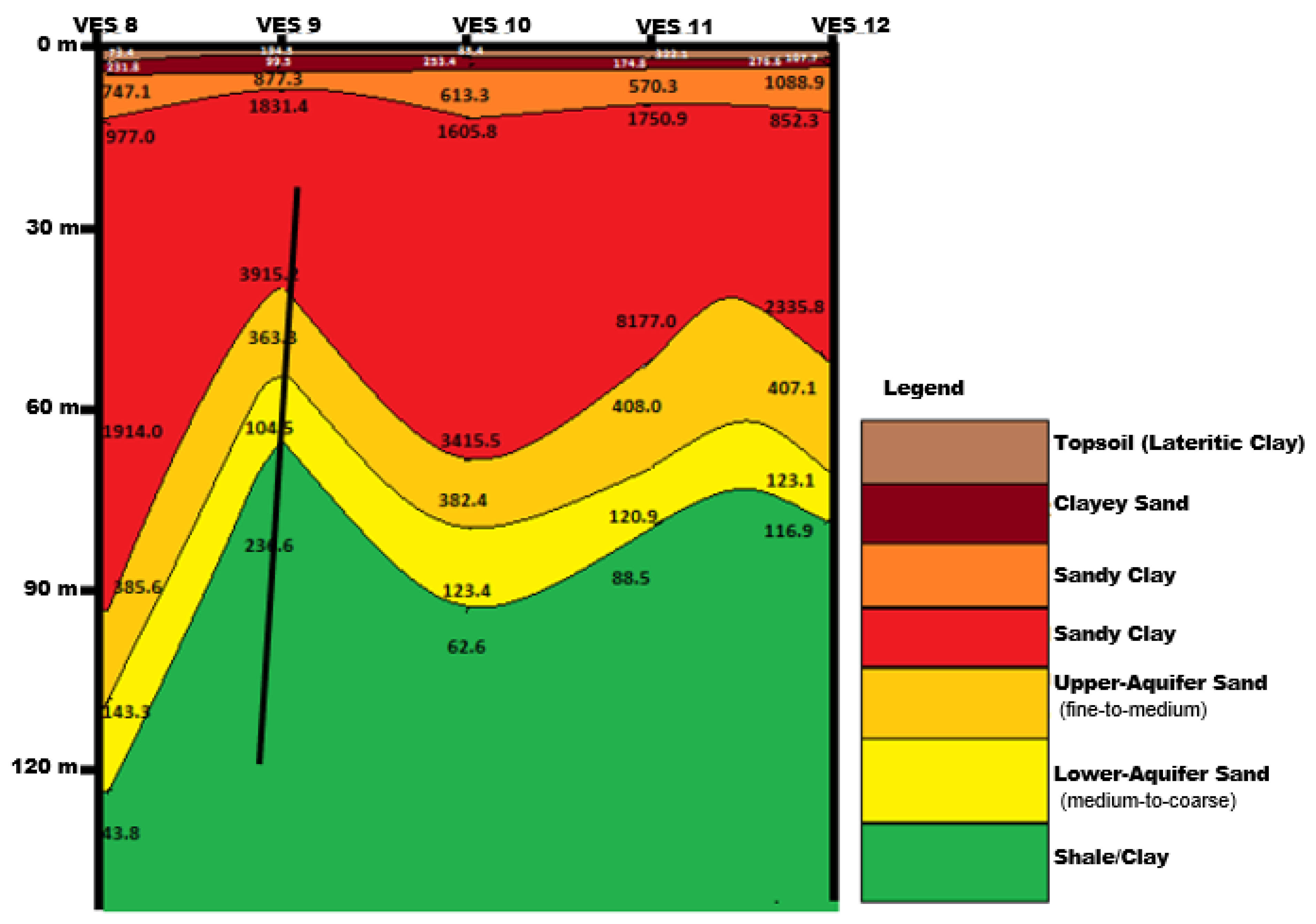
4.1. Vertical Electrical Sounding

The interpretation of the VES data and the geoelectric sections in all the study locations (L1–L5) revealed around eight geoelectrical layers. The estimated geoelectric parameters for the identified geoelectric layers are uniform among all the VES curves, and an example is shown in Table 1. The interpretation of the subsurface lithology from the geoelectric layers at the five locations was established based on the inhomogeneity of electrical resistivity properties and the information from the drilled boreholes and wells integrated with the known local geological setting.
Figure 3 reveals the representative of the inverted VES numbers (1–7) conducted within Covenant University (Location L1). The first geoelectric layer is topsoil, adjudged to be a lateritic clay soil with a resistivity range of 24.5–132.8 Ω m , and a thickness range of 0.9–1.3 m. The topsoil resistivity values are low because it is evident that the layer contains some lateritic clay. The second geoelectric layer shows resistivity values ranging from 119.4–376.7 Ω m , and a thickness range of 1.6–6.5 m that can be interpreted as clayey sand deposits. The third delineated layer with inverse model resistivity values of 399.5–1109.2 Ω m is interpreted as a sandy clay unit with a thickness range of 2.9–19.9 m. The fourth and fifth delineated layers had resistivity ranges of 971.8–2804.8 Ω m and 3102.0–10,341.5 Ω m , and layer thickness ranges of 3.9–8.4 m and 16.0–65.5 m, respectively. This zone is interpreted as a sandy clay layer, which seems to be the confinement of the underlying saturated units. The sixth geoelectric layer has a resistivity range of 347.4–390.1 Ω m , and a layer thickness range of 12.0–15.9 m, and is interpreted as the upper saturated silty sand layer. The seventh delineated layer shows a resistivity range of 119.6–132.0 Ω m , and a thickness range of 11.9–14.2 m and is represented as a lower saturated layer of coarse sand. The last delineated resistivity layer has a resistivity range of 45.7–86.6 Ω m and is interpreted as a shale or clay unit. The summary of the estimated geoelectric parameters from the interpreted VESs is presented in Table 1, and the corresponding geoelectric sections constructed are presented in Figure 4. Two anticipated sub-vertical faults were mapped in the area, as displayed in the geoelectric section.
A total of five VESs were conducted within the Bells University (Location L2) campus, and the interpretation of the VES data equally revealed eight geoelectric strata within the subsurface. The representative inverted VES curves and the resulting model parameters are presented in Figure 5. The first unit of the inverse model shows variable resistivity values in the range 73.4–322.1 Ω m , which is represented by the topsoil of lateritic clay with a thickness range of 0.9–1.9 m. The high resistivity characteristics of the topsoil at some VES points may be attributed to the compaction due to surface activities. The second layer has a resistivity range of 99.5–276.6 Ω m , and a thickness range of 4.4–8.0 m, which can be interpreted as a clayey sand unit. The third layer shows resistivity values of 570.3–1088.9 Ω m and a thickness range of 4.4–8.0 m. This layer is considered a sandy clay unit. The fourth and fifth mapped layers have resistivity ranges of 852.3–1831.4 Ω m and 1914.0–8177.0 Ω m respectively, and the thickness range is 31–83.3 m. This layer can be interpreted as sandy clay and represents the confining bed for the underlying saturated units. The delineated sixth layer has a resistivity range of 363.3–408.0 Ω m and a thickness of 13.1–14.3 m, which can be interpreted as sandy clay. The seventh layer shows a resistivity range of 120.9–143.3 Ω m and a thickness range of 13.0–14.0 m and is interpreted as a medium-to-coarse sand unit. These two zones are expected to be saturated based on the inverted resistivity ranges and the previous geological and hydrological information. This layer overlies a basal shale unit with a resistivity range of 43.8–236.6 Ω m . The constructed geoelectric sections (Figure 6) show a sub-vertical fault based on the sharp changes in the layers’ thicknesses and resistivities.
The representatives of inverted sounding curves for the six VESs conducted along the Oju-Ore-Ilogbo road (location L3) are presented in Figure 7. Like the other locations, eight geoelectric layers were attained for each VES station. The first geoelectric layer is the topsoil, which has a resistivity range of 50.0–138.0 Ω m , and a thickness range of 0.7–1.5 m. The topsoil zone is composed of lateritic clay. The undelayed second layer has a resistivity value range of 39.2–209.1 Ω m and a thickness range of 1.0–2.5 m, which can be interpreted as a clayey sand layer. The third delineated layer is characterised by resistivity values of 187.4–711.6 Ω m and is revealed to be a sandy clay unit with a thickness range of 1.8–3.5 m. The fourth and fifth layers show resistivity ranges of 841.5–3064.5 Ω m and 1119.7–3727.45 Ω m and thickness ranges of 8.4–26.2 m and 17.6–31.7 m, respectively. This zone is interpreted as sandy clay confining the undelayed saturated units. The sixth geoelectric layer is the upper saturated zone in the area, which has a resistivity range of 359.5–404.8 Ω m , and a thickness of 13.6–16.3 m and can be interpreted as a sand saturated layer. The seventh delineated layer is the lower saturated zone, with a resistivity range of 116.3–126.7 Ω m and a thickness of 14.0 m, and represents a saturated sand unit. The mapped basal layer has a resistivity range of 27.7–236.0 Ω m and can be interpreted as the shale layer (Figure 8).
Figure 9 shows the representative of the inverted VES numbers 19–25 conducted along the Obasanjo-Ijagba road (Location L4). Eight subsurface geoelectric layers were interpreted from the sounding data in the area and used to construct the subsurface geoelectric resistivity section (Figure 9). The first layer is the topsoil, which has a resistivity range of 22.5–223.6 Ω m , a thickness range of 0.6–1.7 m, and is interpreted as lateritic clay. The delineated second layer shows resistivity values ranging from 103.7–335.5 Ω m and a thickness of 1.6–3.8 m. It is interpreted as a clayey sand unit. The third delineated layer has a high resistivity value of 414.8–1375.5 Ω m with a thickness range of 4.4–9.8 m, which represents a sandy clay unit. The fourth and fifth delineated layers have high resistivity values of 1187.3–1842.6 Ω m and 2162.5–4064.5 Ω m , and a thickness of 8.5–23.6 m and 15.4–30.4 m, respectively. This unit is represented as highly compacted sandy clay, which is confining the underlying saturated units. The sixth layer shows a resistivity range of 364.5–411.4 Ω m and a thickness range of 13.8–16.1 m, which can be interpreted as the upper saturated silty sand unit. The seventh delineated layer has a resistivity range of 117.5–122.1 Ω m and a thickness ranging from 13.7–14.1 m and represents a lower saturated sand unit. The delineated basal layer shows a resistivity range of 36.0–81.8 Ω m , which can be interpreted as the shale unit (Figure 10).
Five VESs were conducted at Iyana-Iyesi (Location L5), and the interpretation of these soundings data equally revealed eight subsurface geoelectric layers that can be discussed as follows: The representative inverted VES numbers 26–30 curves for the area are presented in Figure 11. Similarly, eight geoelectric layers were delineated, starting with the topsoil, which has variable resistivity values of 53.5–185.4 Ω m with a thickness range of 1.0–1.4 m, representing the lateritic clay layer. The second layer shows resistivity values of 150.8–720.7 Ω m and a thickness of 2.5–3.4 m; this layer represents a clayey sand unit. The third layer has high resistivity values of 796.6–1289.8 Ω m and a thickness range of 5.4–7.4 m, it is interpreted as a sandy clay unit. The fourth and fifth delineated layers have higher resistivity, ranging from 1365.9 to 2179.0 Ω m and 2713.7 to 3885.2 Ω m , and the thickness ranges are 13.5–16.7 m and 21.3–30.8 m, respectively. These layers represent sandy clay units, which are considered the confining beds for the underlying saturated units. The delineated sixth layer has a resistivity range of 368.9–372.6 Ω m and a thickness range of 15.1–15.4 m which represents the silty sand unit, which is considered the upper saturated zone. The seventh layer shows a resistivity range of 120.2–121.3 Ω m and a thickness range of 14.0–14.1 m and is interpreted as a saturated sand unit. This layer overlies a basal shale unit with a resistivity range of 50.1–63.3 Ω m (Figure 12).

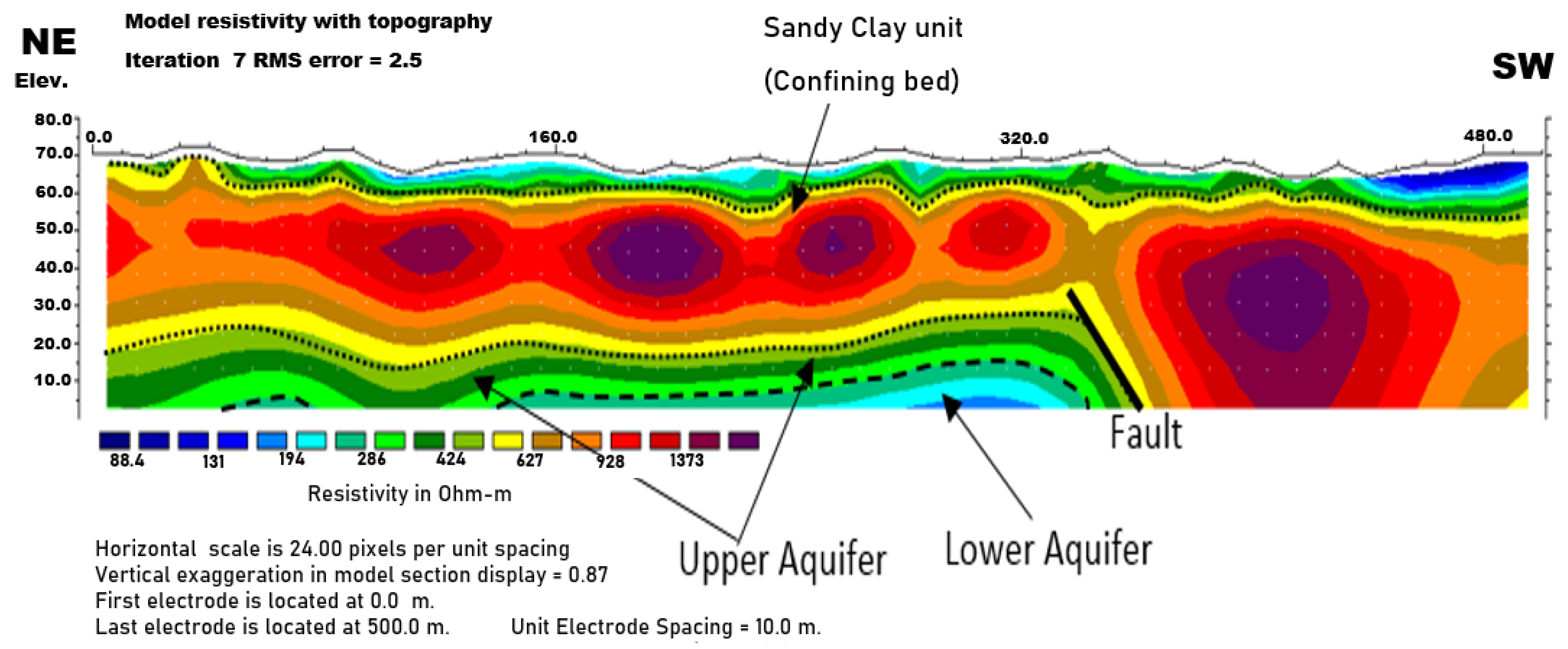
4.2. 2D Electrical Resistivity Imaging

Though both L1-norm and L2-norm inversion techniques were tested for the acquired 2D ERT datasets, only the inverse models using the L2-norm are presented because they better represent the subsurface. The 2D ERT inversion generally reveals the geoelectric layers in more detail and is equivalent to the estimated results using the VESs techniques (Figure 13, Figure 14, Figure 15, Figure 16 and Figure 17). A few iterations were adequate to achieve a good match between the measured and modelled resistivity, and the resulting 2D resistivity section revealed the subsurface layer distribution in relation to the previous geological and VES results. The colour code represents the 2D resistivity distributions, with emphasis on the dry and saturated zones. The inversion of the ERT traverse for location L1 is presented in Figure 13, which reveals the lateral resistivity distribution up to 70 m depth. The 2D ERT profile for traverse T1 shows the presence of the shallow low resistivity layer with resistivities <250 Ω m which represents the clayey topsoil with variable resistivity values according to the surface activities and whose thickness is a maximum of 20 m. This layer is followed by a layer of high resistivity values >800 Ω m with a thickness of 70 m or more. This layer represents the dry sandy clay cap unit, and it is extended along the measured section. The most important unit that appears at elevation 30 m has a low resistivity character, which represents the saturated sandy clay layer. It appears at distinctive locations: at the beginning of the measured profile at 320 m. The sub-vertical sharp resistivity boundaries between the low and high values appear at the beginning and at 330 m horizontal distance, which may be attributed to the presence of a fault (Figure 13).
Similarly, the 2D ERT profile for traverse T2 within Bells University is presented in Figure 14 with the same resistivity value distributions as in T1. The shallow low resistivity layer with resistivities <250 Ω m represents the clayey topsoil with variable resistivity values according to the surface activities, and its thickness is a maximum of 10 m. This layer is followed by a layer of high resistivity values >700 Ω m with a thickness of 60 m and more along the SW direction. This layer represents the dry sandy clay cap unit, and it is extended along the measured section. The most important units that appear at elevation 20 m have a low resistivity character, which represents the saturated sandy clay layer. It appears horizontally along the measured profile and laterally in contact with the high resistivity layer at a horizontal distance of 340 m. This probably reflects the presence of a subvertical fault (Figure 14).
The 2D ERT profile for traverse T3 is presented in Figure 15 and shows similar subsurface resistivity distributions to the previous profiles. Inspecting the inverted resistivity profiles reveals similar subsurface lithological successions in the other two locations. The shallow and thin low resistivity layer with resistivities <250 Ω m represents the clayey topsoil with variable resistivity values. This layer is followed by a layer of high resistivity values >600 Ω m with a thickness of 60 m, thinning in the SE direction. This layer represents the dry sandy clay cap unit, and it is extended along the measured section. The most important units that appear at elevation 0 m have low resistivity, which represents the saturated sandy clay layer. It appears horizontally and smoothly along the measured profile. At the end of the profile, the low resistivity zone (<100 Ω m ) appears underneath the saturated zone. This zone represents the unit bounding the upper saturated layers. (Figure 15). The inverse model of the 2D ERT profile T4 conducted along the Oju-ore-Ilogbo road (location L4) is displayed in Figure 16. Inspecting the inverted resistivity profiles reveals similar subsurface lithological successions to the other 2D profiles. The shallow and thin low resistivity layer with resistivities <220 Ω m represents the clayey topsoil. The second layer has a relatively high resistivity value of >600 Ω m along most of the measured profile with a thickness of about 60–70 m, reflecting the old topography of the underlain sand clay layer. This layer represents the dray sandy clay cap unit, and it is extended along the measured profile. The most important units that appear at elevation 30 m with low resistivity characters represent the saturated sandy clay layer with an irregular bottom topographic surface. At the bottom of the saturated layer, a low resistivity zone (<100 Ω m ) appears, which is interpreted as a shale unit, bounding the upper saturated layers (Figure 16).
The fifth 2D ERT profile is presented in Figure 17, which shows the main subsurface resistivity layer. The shallow and thin low resistivity layer with resistivities <210 Ω m represents the clayey topsoil. This is followed by a high resistivity value > 950 Ω m along most of the measured profile, with a thickness of about 70–80 m along most of the profile. This layer represents the dray sandy clay cap unit, and it is extended along the measured profile except at distances of 230–260 m, where the layer is dissected. The low resistivity character layer appears at elevations of 70 m and 30 m, which represents the saturated sandy clay layer with an irregular topographic surface. At the bottom of the saturated layer, a low resistivity zone (<100 Ω m ) appears, which is interpreted as a shale unit bounding the upper saturated layers (Figure 17).

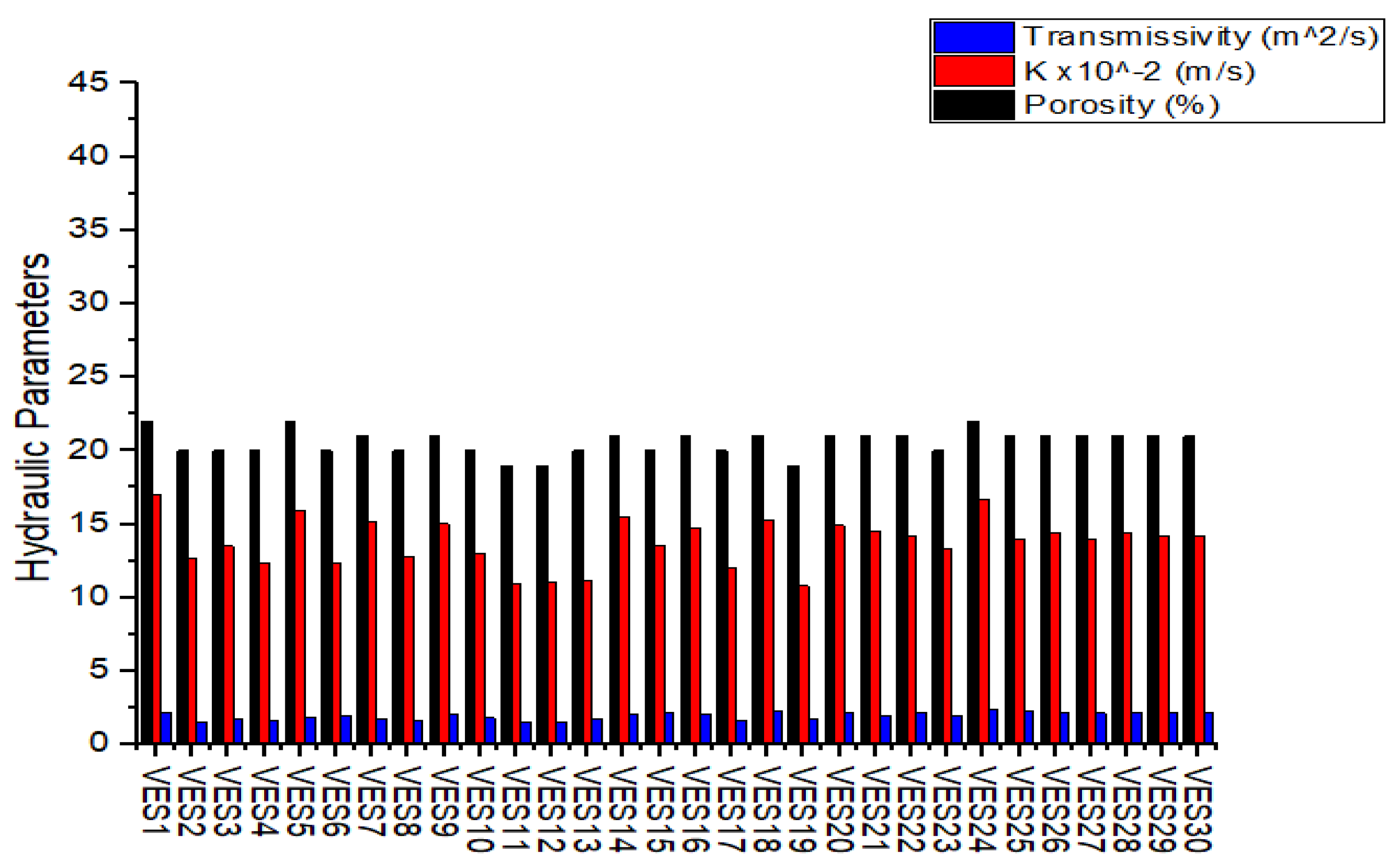
4.3. Aquifers Hydraulic Parameters

Hydraulic parameters play a crucial role in understanding and managing aquifers, which are vital sources of groundwater. To effectively utilise and sustainably manage these invaluable resources, it is essential to accurately estimate hydraulic parameters. Based on the Archie law (Equation (1)), the upper and lower aquifer porosities can be calculated from the interpreted resistivity values deduced from the measured VES stations. Then the Dar Zarrouk parameters (example: Table 1) have been used to calculate the two aquifers’ hydraulic conductivity (Equations (2) and (4)). Using the aquifer thickness, the transmissivity values can be estimated. Table 2 shows the calculated hydraulic parameters for the two aquifers along the five investigated sites. The calculated hydraulic values for the two aquifers at each VES station are presented in Figure 18 and Figure 19. The prediction models for the estimated hydraulic parameters of both upper and lower aquifers are presented in Figure 20 and Figure 21. Equations (6)–(8) are the linear prediction models relating the estimated transmissivity, hydraulic conductivity, and porosity with the mean true resistivity of the upper aquifer. The lower aquifer hydraulic estimated parameters versus mean resistivity values can be expressed in Equations (9)–(11).
M e a n   T r a n s m i s s i v i t y = 6.1993 ( 0.012 ) M e a n   R f
M e a n   K ( 10 2 ) = 54.46 ( 0.011 ) M e a n   R f
M e a n   P o r o s i t y = 0.37 ( 4.37 × 10 4 ) M e a n   R f
The prediction models for hydraulic conductivity and porosity are linear, while the mean transmissivity model is non-linear (3rd-order polynomial). This confirms that the estimated hydraulic values are acceptable for both aquifers.
M e a n     T r a n s m i s s i v i t y = ( 35473.28 ) + 901.36   ( M e a n   R f ) 7.59   ( M e a n   R f ) 2 + 0.021   ( M e a n   R f ) 3
M e a n   K ( 10 2 ) = 1994.623 ( 12.70 ) M e a n   R f
M e a n   P o r o s i t y = 0.85 ( 0.003 ) M e a n   R f

5. Discussion

5.1. Subsurface Characterisation and Aquifer Delineation

The VESs and the 2D electrical resistivity images were integrated for subsurface evaluation up to depths ranging from 90–120 m and delineated the dry and saturated subsurface zones. The geological and borehole information has been considered in the inversion of the VES data sets. Then the borehole and VES models were considered in the inversion and interpretation of the 2D ERT profiles, which show more details about the lateral extension of subsurface layer successions. The delineated geoelectric layers started with the topsoil (mostly lateritic clay), clayey sand, sandy clay, sand, and shale. Most of the interpreted layers are laterally extended along the investigated areas in the same order. On the inverted-sounding data and the 2D ERT sets, the topsoil unit is thin and dominant along most of the surveyed areas. The second dominant layer is the sandy clay unit, which has relatively high resistivity characters across both data sets, with more details about the thickness and continuation appearing in the 2D ERT inverted profiles. The high resistivity character of the sandy clay unit is referred to as the compaction and the clay content, which have been described as being rich in kaolin and intercalated with phosphates. The intercalated phosphates are thought to be part of the reported thin bands of phosphate belonging to the Ilaro Formation [29,32,45]. Despite the resistivity data indicating that this layer is dry, many homeowners tried to hand-dig wells to extract water from this layer with very limited success. Underlain by the high-resistivity clayey sand layer, the low-resistivity characters appear with more details about the layer’s thickness and depth, which are considered saturated with groundwater. This is the sandy clay layer, and based on the geological and borehole information, this unit can be classified into two saturated zones with different grain sizes.
The high resistive unit is confining the unconsolidated sand unit, which forms the upper saturated zone along the study area. It is composed mainly of silty sand deposits. This upper saturated layer is thought to be part of the tertiary alluvium deposits of the Benin Formation [29,32,45]. The lower saturated zone is a coarse-grained sand formation that is perhaps more porous and permeable compared to the upper aquifer system, which is the reason for its lower resistivity characteristics. The lower aquifer is interpreted to be part of the coastal plain sands of the Benin Formation as well. Moreover, many faults were identified by the vertical and sub-vertical sharp contact between the low and high resistivity units. These expected faults penetrate both upper and lower saturated zones at different depths and could scientifically affect sustainable groundwater exploration, development, and management within the two aquifer systems [9,23,46,47].

5.2. Implications for Groundwater Resource Development and Management

The spatial distributions of the true stratigraphic thickness of both the lower and upper saturated zones are presented in Figure 22 and Figure 23. The thickness of an aquifer plays a significant role in groundwater development and management. It determines the storage capacity, sustainability of extraction, water quality, well yield, recharge potential, hydrological dynamics, and adaptability to changing conditions. The thicknesses of both lower and upper saturated zones increase south-westward up to the Iyana-Iyesi area and decrease north-westward down to the Canaan land area (Figure 22 and Figure 23). It denotes the vertical extent of the saturated zone within the aquifer, indicating the depth from which water can be extracted [48]. Aquifer thickness influences its water storage capacity, as a thicker aquifer can store more water, ensuring a larger volume of groundwater available for various uses. The thickness of the aquifer directly influences its sustainable yield, providing a reliable and steady supply of water over an extended period. The estimated hydraulic parameters reveal the productive capacity of the delineated aquifers. Porosity measurements are fundamental to characterising aquifers and understanding their hydrogeological properties. Accurate porosity data are used in groundwater models and simulations to predict aquifer behaviour under different scenarios. It plays a vital role in determining the volume of water that an aquifer can store and transmit. The estimated porosity values range between 20 and 22% within the upper aquifer, while the values range from 48 to 50% for the lower aquifer. The estimated porosity values for both aquifers show their high capacity to store water.
The estimated hydraulic conductivity values of both delineated upper and lower aquifers are high, with values ranging from 12.4–17.0 × 10⁻² m/s for the upper aquifer unit and 371–478 × 10−2 m/s for the lower aquifer unit. Aquifers with high hydraulic conductivity can transmit water more easily, resulting in higher groundwater flow rates. The estimated hydraulic conductivity values of both delineated upper and lower aquifers are high, with values ranging from 1.56–2.18 m2/s for the upper aquifer unit and 50.00–62.14 m2/s for the lower aquifer unit. Understanding the hydraulic conductivity and transmissivity of the subsurface aquifer units is essential for effective groundwater management, water resource planning, and environmental protection. The estimated porosity, hydraulic conductivity, and transmissivity have high values for both delineated major aquifers in the study area.
Moreover, the structural faults within some parts of the study area cut across the delineated aquifers and can have significant impacts on groundwater resource development and management. The faults can serve as conduits for water to enter the aquifer, resulting in increased recharge rates. Groundwater wells may need to be carefully sited to avoid faults, and additional measures may be required to prevent contamination through faults. Thus, it is important to carefully consider the presence of faults when planning groundwater projects and to take steps to mitigate any negative impacts that may result.

6. Conclusions

Groundwater resources have many advantages over surface water, first in terms of comprehensive applications and usability in agriculture, domestic, and manufacturing industries. Thus, there is a need for these natural resources to be appropriately managed and protected to ensure their sustainability. Hydrogeophysical investigations have been employed within the eastern Dahomey basin to provide subsurface information and characterise the multi-layer aquifers within the subsurface. The subsurface lithologic units include the topsoil (Lateritic clay), clayey sand, sandy clay (confining bed), fine-to-medium sand (upper aquifer system), medium-to-coarse sand (lower aquifer system), and shale or clay belonging to the Akinbo Formation, which was delineated in all the locations (L1–L5). The shallower clayey sand and sandy clay formations serve as potential low-yield aquifers that are useful only for hand-dug wells in the study area. Two major aquifers were delineated within the area. The upper aquifer is a fine-silty sand unit with a mean thickness range and mean resistivity range of 13.0–15.3 m and 347.4–389.7 Ω m in the entire area. The estimated hydraulic parameters for the upper aquifer reveal that it is highly productive. The mean porosity range is 20–22%, the mean hydraulic conductivity range is 12.4 × 10⁻² m/s–17.0 × 10−2 m/s, and the mean transmissivity range is 1.56–2.18 m2/s. The delineated lower aquifer is coarse sand, with mean resistivity ranges of 119.6–128.0 Ω m and a mean thickness range of 13.0–14.1 m. The estimated hydraulic parameters for the lower coarse sand aquifer unit have a mean porosity range of 48–50%, a hydraulic conductivity range of 371–478 × 10−2 m/s, and a mean transmissivity range of 50.0–62.14 m2/s. Targeting these aquifers for sustainable groundwater resources during exploration will save the homeowners within the study area from the pain of drilling unproductive and low-yield boreholes. Also, some sub-vertical faults within the study area will affect groundwater resource development and management in the area since the occurrence of these sub-vertical structural faults within the subsurface will result in changes in the permeability of the delineated aquifers across the divide, thereby affecting the productivity of the aquifer units in the area. There is a need to establish an hydrogeophysics observatory in the study area to obtain time-lapse hydrogeological data such as groundwater level data, pumping test data, groundwater recharge rate, and groundwater quality data. Integrating these data with the findings of this research would enable the building of effective groundwater models of the delineated, multi-layered aquifers in the area. With robust groundwater models of the aquifers, managed aquifer recharge (MAR) projects will be effective in the area to sustain groundwater supply. Moreover, there is a need to understand groundwater flow and transport processes within the delineated aquifer systems in the area to predict the movement and fate of contaminants in the aquifer. This is crucial for managing and mitigating the impacts of groundwater pollution, protecting water quality, and safeguarding public health in the area.

Author Contributions

Conceptualization, K.D.O., A.P.A. and M.M.; methodology, K.D.O., A.P.A., A.A.O. and D.V.K.; software, E.E.O., D.V.K. and M.M.; validation, A.P.A., K.D.O., A.A.O. and M.M.; formal analysis, K.D.O., A.A.O. and A.P.A.; field investigation, K.D.O., E.E.O., A.A.O. and A.P.A.; resources, D.V.K. and M.M.; data curation, K.D.O. and A.P.A.; writing—original draft preparation, K.D.O., A.A.O. and E.E.O.; writing—review and editing, K.D.O. and M.M.; supervision, A.P.A. and M.M.; project administration, A.P.A. and K.D.O.; funding acquisition, M.M. All authors have read and agreed to the published version of the manuscript.

Funding

This work was funded by the Deputyship for Research and Innovation, “Ministry of Education” in Saudi Arabia (IFKSUOR3-093-1).

Data Availability Statement

Not applicable.

Acknowledgments

The authors wish to express their appreciation to the Deputyship for Research and Innovation, “Ministry of Education” in Saudi Arabia for funding this research (IFKSUOR3-093-1). Also, the authors appreciate the Covenant University Center for Research, Innovation, and Development (CUCRID) for the research support. The first author is thankful to both UNESCO-TWAS and CSIR, India, for the CSIR-TWAS Postdoctoral Fellowship at the National Geophysical Research Institute, India.

Conflicts of Interest

The authors declare no conflict of interest.

References

  1. Barlow, J.R.B.; Clark, B.R. Simulation of Water-Use Conservation Scenarios for the Mississippi Delta Using an Existing Regional Groundwater Flow Model: U.S. Geological Survey Scientific Investigations Report 2011–2019; U.S. Geological Survey: Reston, VA, USA, 2011; 14p. [Google Scholar]
  2. UNESCO. Water a Shared Responsibility. The United Nations World Water Development Report 2; UNESCO: New York, NY, USA, 2006; p. 601. [Google Scholar]
  3. WHO/UNICEF. Water for Life. Making it Happen. A Decade for Action 2005–2015; WHO: Geneva, Switzerland, 2005; p. 44. [Google Scholar]
  4. Rubin, Y.; Hubbard, S.S. Hydrogeophysics, Water Science and Technology Library; Springer: New York, NY, USA, 2005. [Google Scholar]
  5. Nwankwoala, H.O.; Udom, G.J. Influence of land reclamation on the status of groundwater in Borokiri area of Port Harcourt, Niger Delta, Nigeria. Int. J. Nat. Appl. Sci. 2008, 4, 431–434. [Google Scholar] [CrossRef]
  6. Kaya, M.A.; Ozürlan, G.S.; Engül, E. Delineation of soil and groundwater contamination using geophysical methods at a waste disposal site in çanakkale, Turkey. Environ. Monit. Assess. 2007, 135, 441–446. [Google Scholar] [CrossRef] [PubMed]
  7. Balkaya, Ç.; Kaya, M.A.; Goktürkler, G. Delineation of shallow resistivity structure in the city of Burdur, SW Turkey by vertical electrical sounding measurements. Environ. Geol. 2009, 57, 571–581. [Google Scholar] [CrossRef]
  8. Olaojo, A.A.; Oladunjoye, M.A.; Sanuade, O.A. Geoelectrical assessment of polluted zone by sewage efflent in University of Ibadan campus southwestern Nigeria. Environ. Monit. Assess. 2018, 190, 24. [Google Scholar] [CrossRef] [PubMed]
  9. Oyeyemi, K.D.; Aizebeokhai, A.P.; Ndambuki, J.M.; Sanuade, O.A.; Olofinade, O.M.; Adagunodo, T.A.; Olaojo, A.A.; Adeyemi, G.A. Estimation of aquifer parameters from surficial geophysical methods: A case study of Ota, Southwestern Nigeria. IOP Conf. Ser. Earth Environ. Sci. 2018, 173, 012028. [Google Scholar] [CrossRef]
  10. Oyeyemi, K.D.; Abuka-Joshua, J.; Rotimi, O.J.; Dieppos, B.; Gomo, M.; Olaojo, A.A.; Falae, P.O.; Metwaly, M. Geoelectrical Characterization of Coastal Aquifers in Agbado Ijaye, Lagos, Southwestern Nigeria; Implications for groundwater resources. Sustainability 2023, 15, 3538. [Google Scholar] [CrossRef]
  11. Sendrós, A.; Himi, M.; Lovera, R.; Rivero, L.; Garcia-Artigas, R.; Urruela, A.; Casas, A. Geophysical Characterization of Hydraulic Properties around a Managed Aquifer Recharge System over the Llobregat River Alluvial Aquifer (Barcelona Metropolitan Area). Water 2020, 12, 3455. [Google Scholar] [CrossRef]
  12. Mohammed, M.A.A.; Abdelrahman, M.M.G.; Szabó, N.P.; Szűcs, P. 2023. Innovative hydrogeophysical approach for detecting the spatial distribution of hydraulic conductivity in Bahri city, Sudan: A comparative study of Csókás and Heigold methods. Sustain. Water Resour. Manag. 2023, 9, 107. [Google Scholar] [CrossRef]
  13. Mohammed, M.A.A.; Szabó, N.P.; Szűcs, P. Characterization of groundwater aquifers using hydrogeophysical and hydrogeochemical methods in the eastern Nile River area, Khartoum State, Sudan. Environ. Earth Sci. 2023, 82, 219. [Google Scholar] [CrossRef]
  14. Szabó, N.P.; Kormos, K.; Dobróka, M. Evaluation of hydraulic conductivity in shallow groundwater formations: A comparative study of the Csókás’ and Kozeny–Carman model. Acta Geod. Geophys. 2015, 50, 461–477. [Google Scholar] [CrossRef] [Green Version]
  15. Hasan, M.; Shang, Y.; Jin, W.; Akhter, G. Estimation of hydraulic parameters in a hard rock aquifer using integrated surface geoelectrical method and pumping test data in southeast Guangdong, China. Geosci. J. 2021, 25, 223–242. [Google Scholar] [CrossRef]
  16. El Osta, M.; Masoud, M.; Badran, O. Aquifer hydraulic parameters estimation based on hydrogeophysical methods in West Nile Delta, Egypt. Environ. Earth Sci. 2021, 80. [Google Scholar] [CrossRef]
  17. Benabdelouahab, S.; Salhi, A.; Himi, M.; Stitou El Messari, J.E.; Ponsati, A.C. Geoelectrical investigations for aquifer characterization and geoenvironmental assessment in northern Morocco. Environ. Earth Sci. 2019, 78, 209. [Google Scholar] [CrossRef]
  18. Nemer, Z.; Khaldaoui, F.; Benaissa, Z.; Belaroui, A.; Tebbouche, M.Y.; Ydri, A. Hydrogeophysical investigation of aquifer parameters and seawater intrusion: A case study from Eastern Mitidja plain, Algeria. Geomech. Geophys. Geo-Energy Geo-Resour. 2023, 9, 60. [Google Scholar] [CrossRef]
  19. Singh, S.; Tripura, J. Combined ERT survey and pumping test for correlation analysis of geoelectrical and aquifer parameters in hilly terrain. J. Earth Syst. Sci. 2023, 132, 43. [Google Scholar] [CrossRef]
  20. Ha, D.; Zheng, G.; Zhou, H.; Zeng, C.; Zhang, H. Estimation of hydraulic parameters from pumping tests in a multiaquifer system. Undergr. Space 2020, 5, 210–222. [Google Scholar] [CrossRef]
  21. Fleming, S.W.; Vesselinov, V.V.; Goodboy, A.G. Augmenting geophysical interpretation of data-driven operational water supply forecast modelling for a western US river using a hybrid machine learning approach. J. Hydrol. 2021, 597, 126327. [Google Scholar] [CrossRef]
  22. Aizebeokhai, A.P.; Oyebanjo, O.A. Applications of vertical electrical soundings to characterize aquifer potential in Ota, Southwestern Nigeria. Int. J. Phys. Sci. 2013, 8, 2077–2085. [Google Scholar]
  23. Aizebeokhai, A.P.; Oyeyemi, K.D.; Joel, E.S. Groundwater potential assessment in a sedimentary terrain, southwestern Nigeria. Arab. J. Geosci. 2016, 9, 496. [Google Scholar] [CrossRef]
  24. Adewumi, I.K.; Ogbiye, A.S.; Longe, E.O.; Omole, D.O. Effects of industrial effluents on water quality of River Atuwara in Ota, Nigeria. In Urban Agriculture, Cities, and Climate Change; Adeyemi, R., Ed.; Cuvallier: Gottinger, Germany, 2011; ISBN 978-3-86955-813-4. [Google Scholar]
  25. Omole, D.O. Reaeration Coefficient modelling: Case study of River Atuwara, Ota, Nigeria. Res. J. Appl. Sci. Eng. Technol. 2012, 4, 1237–1243. [Google Scholar]
  26. Adewuyi, G.B.; Badejo, O.T.; Idowu, F.F.; Ogunjobi, G.A.; Gbopa, A.O. Analysis of Physico-chemical parameters: An emperical study of Yewa River, Ogun state and part of Badagry creek, Lagos, Southwestern Nigeria. Int. J. Hydrol. 2017, 2, 36–46. [Google Scholar]
  27. Omatsola, M.E.; Adegoke, S.O. Tectonic Evaluation and Cretaceous Stratigraphy of the Dahomey Basin. Niger. J. Min. Geol. 1981, 18, 130–137. [Google Scholar]
  28. Jones, H.A.; Hockey, R.D. The geology of part of south western Nigeria. Geol. Surv. Niger. Bull. 1964, 31, 1–101. [Google Scholar]
  29. Ako, B.D.; Adegoke, O.S.; Petters, S.W. Stratigraphy of Oshoshun Formation in southwestern Nigeria. Nig. J. Min. Geol. 1980, 17, 99–106. [Google Scholar]
  30. Okosun, E.A. A review of the cretaceous stratigraphy of the Dahomey embayment, west Africa. Cretac. Res. 1990, 11, 17–27. [Google Scholar] [CrossRef]
  31. Elueze, A.A.; Nton, M.E. Organic geochemical appraisal of limestones and shales in part of eastern Dahomey basin, southwestern Nigeria. J. Min. Geol. 2004, 40, 29–40. [Google Scholar] [CrossRef]
  32. Adegoke, S.O.; Dessauvagie, T.F.J.; Whitman, A.J. Macrofauna of Ewekoro Formation (Paleocene) of Southwest Nigeria; African Geology; University of Ibadan: Ibadan, Nigeria, 1970; pp. 269–276. [Google Scholar]
  33. Gebhardt, H.; Adekeye, O.A.; Akande, S.O. Late Paleocene to initial Eocene thermal maximum foraminifera biostratigraphy and paleoecology of the Dahomey basin, southwestern Nigeria. Gjahrbuch Der Geologischem. Bundesantalt 2010, 150, 407–419. [Google Scholar]
  34. Griffiths, D.H.; Barker, R.D. Two-dimensional resistivity imaging and modelling in area of complex geology. J. Appl. Geophys. 1993, 29, 211–226. [Google Scholar] [CrossRef]
  35. Smith, D.L.; Ritter, D.F. Groundwater Geophysics: A tool for hydrogeology. Geophys. Explor. Eng. Environ. Investig. 2003, 18, 15–42. [Google Scholar]
  36. Dabas, M.; Taritis, P.; Hallouin, T. Interpretation of Geophysical Data. In Treatise of Geophysics, 2nd ed.; Archie, G.E., Logan, J.D., Richardson, M.H., Eds.; Elsevier: Amsterdam, The Netherlands, 2011; Volume 2, pp. 523–553. [Google Scholar]
  37. Minsley, B.J.; Sweeney, R.E.; Slater, L.D. Estimating Hydraulic conductivity with geophysicsical data: What’s Feasibl? Vadose Zone J. 2007, 6, 167–179. [Google Scholar]
  38. Auken, E.; Christiansen, A.V. Layered and Laterally constrained 2D inversion of resistivity data. Geophysics 2005, 70, G49–G59. [Google Scholar] [CrossRef]
  39. Archie, G. The electrical resistivity log as an aid in determining some reservoir characteristics. Pet. Trans. Am. Inst. Mineral. Metall. Eng. 1942, 146, 54–62. [Google Scholar] [CrossRef]
  40. Archie, G. Introduction to petrophysics of reservoir rocks. AAPG Bull. 1950, 34, 943–961. [Google Scholar]
  41. Lynch, E.J. Formation Evaluation; Harper and Row Publishers Inc.: New York, NY, USA, 1964. [Google Scholar]
  42. Kozeny, J. Hydraulics; Springer: Vienna, Austria, 1953. [Google Scholar]
  43. Carman, P.C. Fluid Flow through granular beds. Trans. Inst. Chem. Eng. 1937, 15, 150–166. [Google Scholar] [CrossRef]
  44. Fogg, G.E.; Noyes, C.D.; Carle, S.F. Geologically based model of heterogeneous hydraulic conductivity in an alluvial setting. Hydrogeol. J. 1998, 6, 131–143. [Google Scholar] [CrossRef]
  45. Olabode, S.O. Silclastics slope deposits from the Cretacious Abeokuta group, Dahome (Benin) basin, southwestern Nigeria. J. Afr. Earth Sci. 2006, 46, 187–200. [Google Scholar] [CrossRef]
  46. Aizebeokhai, A.P.; Oyeyemi, K.D. The use of the multiple gradient array for geoelectric resistivity and induced polarization imaging. J. Appl. Geophys. 2014, 111, 364–376. [Google Scholar] [CrossRef]
  47. Aizebeokhai, A.P.; Oyeyemi, K.D. Application of geoelectrical resistivity imaging and VLF-EM for subsurface characterization in a sedimentary terrain, southwestern Nigeria. Arab. J. Geosci. 2015, 8, 4083–4099. [Google Scholar] [CrossRef]
  48. Kumar, T.J.R.; Balasubramanian, A.; Kumar, R.S.; Dushiyanthan, C.; Thirumeelakandan, B.; Suresh, R.; Karthikeyan, K.; Davidraju, D. Assessment of groundwater potential based on aquifer properties of hard rock terrain in the Chittar-Uppodai watershed, Tamil Nadu, India. Appl. Water Sci. 2016, 6, 179–186. [Google Scholar] [CrossRef] [Green Version]
Figure 2. The dominant lithological succession along the study area deduced from the borehole log data for the location refers to Figure 1.
Water 15 02862 g002
Figure 3. Representative of the inverted VES curves within Covenant University (L1) and the resulting digital subsurface models.
Water 15 02862 g003aWater 15 02862 g003b
Figure 4. Geoelectric subsurface section from sounding results carried out along the Covenant University, showing the inferred faults.
Water 15 02862 g004
Figure 5. Representative of the inverted VES curves within Bells University (L2) and the resulting digital subsurface models.
Water 15 02862 g005aWater 15 02862 g005b
Figure 6. Geoelectric subsurface section from sounding results carried out along the Bells University, showing the inferred faults.
Water 15 02862 g006
Figure 7. Representative of the inverted VES curves within Oju-Ore-Ilogbo Road (L3) and the resulting digital subsurface models.
Water 15 02862 g007
Figure 8. Geoelectric subsurface section from sounding results carried out along Oju-Ore-Ilogbo Road.
Water 15 02862 g008
Figure 9. Representative of the inverted VES curves within Obasanjo-Ijagba Road (L4) and the resulting digital subsurface models.
Water 15 02862 g009aWater 15 02862 g009b
Figure 10. Geoelectric subsurface section from sounding results carried out along Obasanjo-Ijagba road.
Water 15 02862 g010
Figure 11. Representative of the inverted VES curves within Iyana-Iyesi (L5) and the resulting digital subsurface models.
Water 15 02862 g011
Figure 12. Geoelectric subsurface section from sounding results carried out along the Obasanjo-Ijagba road.
Water 15 02862 g012
Figure 13. 2D subsurface geoelectrical resistivity image for traversing T1 Covenant University; dashed lines delineate the boundaries between the different layers. The solid lines are the fault locations.
Water 15 02862 g013
Figure 14. 2D subsurface geoelectrical resistivity image for traverse T2 at Bells University.
Water 15 02862 g014
Figure 15. Two–dimensional geoelectrical resistivity image for traverse T3 along the Oju-Ore-Ilogbo road (L3).
Water 15 02862 g015
Figure 16. Two-dimensional geoelectrical resistivity image for traverse T4 along the Obasanjo-IJagba road (L4).
Water 15 02862 g016
Figure 17. Two-dimensional geoelectrical resistivity image for traverse T5 at Iyana-Iyesi (L5).
Water 15 02862 g017
Figure 18. Estimated porosity, hydraulic conductivity, and transmissivity for the upper aquifer were deduced from the measured- VES stations.
Water 15 02862 g018
Figure 19. Estimated porosity, hydraulic conductivity, and transmissivity for lower aquifer were deduced from the measured- VES stations.
Water 15 02862 g019
Figure 20. Predicted model for mean transmissivity of upper aquifer from the true mean resistivity.
Water 15 02862 g020
Figure 21. Predicted model for mean transmissivity of the lower aquifer from the true mean resistivity.
Water 15 02862 g021
Figure 22. Spatial distribution of the Upper aquifer thickness in meters.
Water 15 02862 g022
Figure 23. Spatial distribution of the Lower aquifer thickness in metres.
Water 15 02862 g023
Table 1. Example of the estimated parameters for VES data sets along the Covenant University (L1) that were utlised to construct the Geoelectric resistivity sections.
VES Layer 1Layer 2Layer 3Layer 4Layer 5Layer 6Layer 7Layer 8
LithologyLateritic ClayClayey SandSandy ClaySandy ClayFine Silty-Sand
(Upper aquifer)
Coarse Sand (Lower aquifer)Shale/Clay
1Resistivity89142.81039.31543.93107.6347.4125.486.6
Thickness1.32.44.68.41612.812.5
Depth1.33.88.316.832.745.558
2Resistivity83.5241.2782.71034.53209.5386.712148.5
Thickness1.1246.741.212.312.1
Depth1.13.17.113.85567.379.3
3Resistivity108.9214.2915.22628.810,341.50378.5119.645.7
Thickness12.13.43.92313.113
Depth13.16.510.433.446.559.5
4Resistivity51.7222.7874.1980.25994.2389.7120.847.4
Thickness0.91.65.68.34513.513.5
Depth0.92.68.216.561.57588.1
5Resistivity24.5376.7399.5971.83102356.212834.1
Thickness0.96.519.98221213.9
Depth0.97.427.235.357.369.283.2
6Resistivity59.3287.21109.21355.69784.1390.113283.6
Thickness12.87.320.165.515.914.2
Depth13.811.131.296.7112.7126.9
7Resistivity132.8119.4508.52804.85817.9361.6119.936.7
Thickness13.92.95.618.311.811.9
Depth14.97.813.431.743.455.3
Table 2. Estimated hydraulic parameters for upper and lower aquifers in the study area.
Upper AquiferLower Aquifer
LocationMean RF
Ω-m
Mean
Porosity
Mean K
(m/s)10−2
Mean T
(m2/s)
Mean RF
Ω-m
Mean
Porosity
Mean K
(m/s)10−2
Mean T
(m2/s)
L1(V1–V7)347.40.218217.02.18125.40.477740050.00
L2(V8–V12)386.70.200912.71.56121.00.491045755.30
L3(V13–V18)378.50.204213.51.76119.60.495547862.14
L4(V19–V25)389.70.199712.41.68120.80.491746062.10
L5(V26–V30)356.20.214015.91.90128.00.470337151.57
Disclaimer/Publisher’s Note: The statements, opinions and data contained in all publications are solely those of the individual author(s) and contributor(s) and not of MDPI and/or the editor(s). MDPI and/or the editor(s) disclaim responsibility for any injury to people or property resulting from any ideas, methods, instructions or products referred to in the content.

