Runoff Simulation and Climate Change Analysis in Hulan River Basin Based on SWAT Model

Abstract

The shortage of water resources is a long-standing constraint on the development of the Chinese economy and society. In this paper, the climate change occurring in Hulan River Basin is analyzed using the data collected at Wangkui Meteorological Station from 1960 to 2020. The overall temperature in the basin shows an upward trend, with a cumulative increase of 1.6 °C, as does the precipitation, which reaches 566.2 mm. In contrast, there is a downward trend shown by wind speed, with a cumulative decrease of 1.313 m/s. GIS remote sensing technology is applied to build a SWAT distributed hydrological model for the purpose of conducting runoff simulation in Hulan River Basin, and SWAT-CUP software is used to correct and analyze the simulation results. The parameters of snow melt are set to improve the accuracy of the model. The runoff data collected from Lanxi Hydrological Station from 2008 to 2020 are used to verify the model. The results show that the efficiency coefficient (NES) and correlation coefficient (R²) are 0.75 and 0.84, respectively, in the validation period from 2010 to 2013, while they are 0.77 and 0.93, respectively, in the correction period from 2014 to 2016, meeting the criteria of model evaluation. It can be seen from results noted above that SWAT is applicable in Hulan River Basin, providing a certain reference for the management of hydrological and water resources available in this region and for the construction of a distributed hydrological model of rivers in those high-latitude cold regions.

1. Introduction

A distributed hydrological model plays an important role in the study of hydrological, ecological, environmental and other issues in a given basin [1]. For this reason, such models have been widely used to quantitatively assess the impact of climate change on water resources [2]. In addition, hydrological models lay a foundation for the exploration of the relationship between soil and hydrology [3]. With the development of social economy, the approaches to spatial data acquisition have been constantly improved, such as geographic information systems, remote sensing imaging and radar. A variety of distributed hydrological models, including SWAT, IHDM, TOPMODEL, etc., have also been widely applied. [4]. Independently developed by the United States Department of Agriculture based on ArcGIS software [5], the SWAT model (Soil and Water Assessment Tool) [6] is the most widely used watershed-scale model worldwide [7,8,9,10] and is capable of producing satisfactory simulation results [11,12]. With different data as the input, the SWAT model is applicable to areas lacking in data and can be used to analyze the hydrological characteristics, soil change characteristics and transfer of chemical pollutants and sediment in a basin through simulation and to reflect the response of human activities and climate change to the runoff characteristics of the basin [13,14,15]. As a development tool based on soil, meteorology, vegetation, hydrology and other characteristics of North America, the SWAT model can be applied to multiple river basins [16]. Before its application, a complete spatial database [17,18] must be established according to the exact conditions in the study area for improved analysis and prediction of future changes, including digital elevation maps, land use maps, topographic maps, feature information, geological structure maps, etc.

Although this model was developed in the United States, many experts and scholars in China have adopted SWAT to analyze different river basins across the country. Nina Omani [19] improved the snow parameter algorithm of the SWAT model and evaluated and improved the previous effect, demonstrating the improved performance in snowmelt runoff simulation in winter. Majed Abu-Zreig [20] used the SWAT model to simulate the Yarmuk River Basin (Jordan) to evaluate the applicability of SWAT to an arid river basin. Ultimately, R² = 0.95 and NES = 0.96 were determined, indicating the excellent performance of the SWAT model in simulating the Jordan dry land basin. Ajay Ratna Bajracharya [21] used not only the SWAT model to simulate the hydrological environment of the Kali Kandaki Basin in Nepal but also the general circulation model of Wing Loong (CMIP4) to simulate future climate change in this basin. According to the results, the critical influencing factors for water balance in the upper Kali Kandaki Basin and the high-altitude areas of the Neutron Basin, such as snowmelt, evapotranspiration and water production, were most affected by the rise in moderate atmospheric precipitation. Githui et al. [22] assessed the impact of climate change on simulated runoff using the SWAT model in western Kenya, with the results showing that an increase in average annual rainfall from 2.4% to 23.2% led to a sharp rise in runoff from about 6% to 115%. In addition, Lucas applied the SWAT model to analyze the effects of different types of land use and climate on the surface runoff in tropical forest basins in Brazil [23].

For the rivers in high-latitude cold regions across China, the study areas for runoff simulation based on the SWAT model concentrate in the middle and upper reaches of the Yellow River Basin [24,25,26]. Due to the scarcity of meteorological stations, however, few studies have been conducted on the rivers in northeast China. In this study, the climate change occurring in Hulan River Basin from 1960 to 2020 is analyzed through the linear analysis and anomaly method, the SWAT model is used to simulate runoff and the SWAT-CUP model is used to assess the simulation results for the improved longitude of the model.

2. Study Area and Data Sources

2.1. Study Area Overview and Data Acquisition

2.1.1. Study Area Profile

The Hulan River, located in the center of Heilongjiang Province, China, is one of the widest tributaries of Heilongjiang River and a major tributary on the right bank of the Songhua River. The basin is about 7240 km long from north to south, 210 km wide from east to west and 520 km long from the main stream, covering an area of 35,683 km² [27]. Geographically, it is located between 125°55′~128°43′ east longitude and 45°52′~48°03′ north latitude in Figure 1. Originating from Lublow Mountain, Hulan River is located at the southwestern foot of the Lesser Khingan Mountains, upstream and 3 km to the west of Taoshan. The river flows through the Hulan District of Harbin City. The overall terrain is high in the northeast but low in the southwest. Mountains and hills account for 59% of the total area, while plains account for 41%. The local climate is characterized by long, dry winters and short, wet summers, which shape a typical river in the high-latitude cold area.

2.1.2. Acquisition of DEM Data in the Watershed

In the SWAT model, DEM data offer crucial support for both the operation of the model and hydrological analysis. Therefore, DEM data are among the first to be downloaded and inputted into the model. In the present study, the ASTRE GDEM 30 M digital elevation model is used to provide DEM information, which is collected from the geospatial databases in http and (gscloud.cn). The meteorological data collected at Wangkui Meteorological Station from 1960 to 2020 are accessed through the China Meteorological Data Network (cma.cn). The elevation of the research area ranges between 7 and 827 m, as shown in Figure 2.

2.1.3. Access to Watershed Land Use Data

The land use data are sourced from the National Qinghai-Tibet Plateau Science Center (TPDC) with a resolution of 30 M. The land use map is shown in Figure 3. The land type code is consistent with the land data of the SWAT model, whose classification number is shown in

Table 1. Land use data.

Number	Land Type	SWAT Coding	Area (Km²)	Proportion (%)
1	Arable land (general)	AGRL	11,909.5675	72.07
2	Forest land	FRST	1852.4525	11.21
3	Meadow	PAST	277.62	1.68
4	Water	WATER	380.075	2.3
5	Residential area	UBRN	1414.54	8.56
6	Wasteland	SWRN	550.2825	3.33
Total			16,525	100

.

2.1.4. Access to the Data on Watershed Land Use

Soil type data are obtained from Harmonized World Soil Database (HWSD), and soil types are classified according to the FAO-90* classification system. According to the HWSD, the total number of soil types in the study area ranges from 11,112 to 11,929. All soil types are reclassified according to area proportion, with nine different soil types determined. The reclassification results are shown in Figure 4, and the soil types are listed in

Table 2. Soil type classification.

Label	Soil Type (HWSD)	Name	Area (Km²)	Proportion (%)
11,112	PHh	Simple black soil	12,484.6375	75.55
11,141	CHg	Gley chernozem	1736.7775	10.51
11,341	FLc	Calcareous alluvial soil	1.1898	0.0072
11,359	GLk	Calcium gley soil	128.6306	0.7784
11,637	ATc	Anthropogenic soil	378.753	2.292
11,917	LVa	Bleached highly active leucosote	1558.4728	9.431
11,925	UR	Urban industrial and mining areas	123.8714	0.7496
11,928	WR	Water	110.767	0.6703
11,929	DS	Dune shifting sand	0.5949	0.0036
Total			16,525	100

.

After processing of all the data and databases, the SWAT model simulation is carried out to create hru, rch and sub3 data tables. The Watershed Delineator in the model is inputted into DEM data for the construction of the river network. Then, the watershed outlet is delineated to reach the conclusion that the watershed consists of 29 sub-basins. SWAT-CUP was developed in 1994 by Dr. Jeff Arnold of the Agricultural Research Center of the United States Department of Agriculture (USDA). It is used to analyze the data runoff simulation. Lansi Hydrographic Station is located at sub9 of the subbasin.

3. Methodology

3.1. Time Series Analysis

The precipitation and temperature meteorological factors are transformed into time series, and the trend of changes in each factor over time is analyzed by means of linear fitting. Thus, a unitary linear regression equation is established as follows:

$$x_i=a{t}_i+b$$

(1)

where a represents the linear regression coefficient, of which a positive or negative value indicates an increasing or decreasing trend of its influence factor, respectively; b denotes the regression constant; a and b refer to the fitting parameters of the least squares method, whose calculation formula is expressed as follows:

$$a=\frac{n\sum x_i{y}_i-\sum x_i{y}_i}{n\sum x^2-\left({\sum x}_i\right)²}$$

$$b=\frac{\sum y_i}{n}-a\frac{\sum x_i}{n}$$

(2)

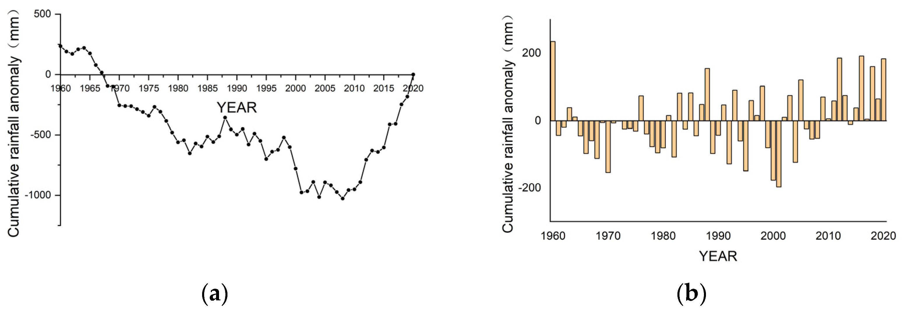
3.2. Anomaly Method and Cumulative Anomaly Method

For long series of meteorological data, the anomaly method is commonly used to determine the data for a certain period or time relative to a long-term average of the data (such as the 30-year average), i.e., relatively high or low, and the original value is generally used to reflect the actual level of a specific period. Cumulative anomalies are also known as the accumulation of anomalies. The main step is to define a set of variables $(x_1,x_2\dots \dots x_n)$, find the mean ($\overline{x}$), then subtract each x from the mean, which is $x_i-\overline{x}$. The corresponding time of the variable is denoted as$t_i$. The sum of all anomalies should be obtained before $t_i$, and ${\sum }_{i=1}^t(x_i-\overline{x})$ is the cumulative anomaly. After the curve of cumulative anomaly over time is drawn, the upward or downward trend of long-term evolution is judged through the fluctuation of the curve change.

3.3. The Soil and Water Assessment Tool (SWAT) Model

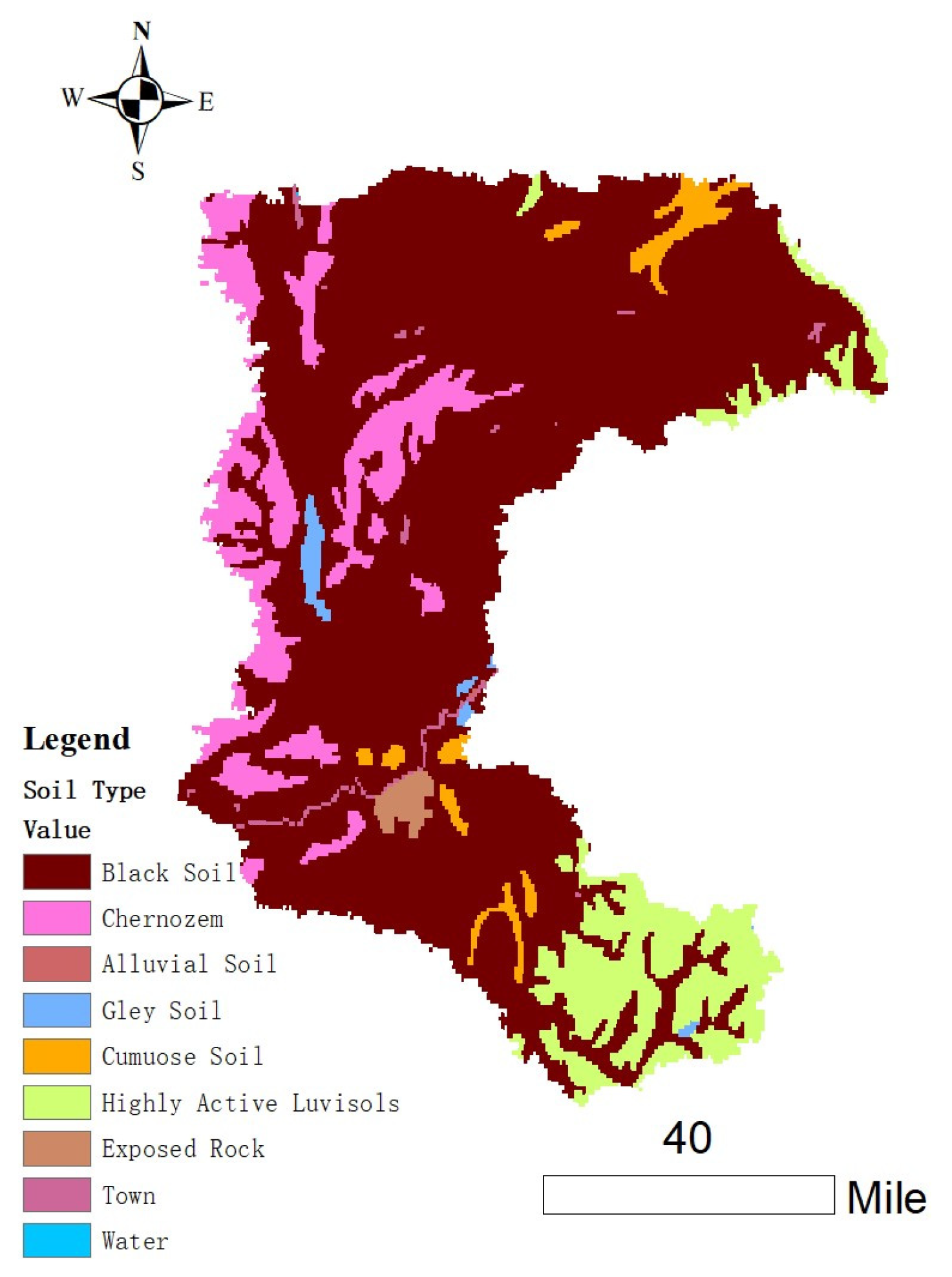
3.3.1. Construction of Soil Database

There are more than 10 types of soil data needing to be inputted into the SWAT model, including hydrological unit group parameters, soil stratification number, soil wet density, water capacity, soil erosivity factor, etc.

Hydrological and soil composition represents one of the most important parameters for the SWAT model when the SCS runoff curve number model is used to simulate water flow. According to the Environmental Protection Agency, soil with a similar capacity of water flow is classified into four categories: A, B, C and D. All four types of soil are similar in precipitation and surface characteristics. Among them, A, B, C and D correspond to four types of soil with permeability ranked from high to low, respectively [28]. The specific rules of soil hydrology group are divided according to the calculated SOL_K (saturated water conductivity) value, as shown in

Table 3. Definition of SWAT model soil hydrological classification (HYDGRP).

Type	Minimum Infiltration Rate (mm/h)	Permeability	Soil Texture
A	>7.26	Higher	Sandy soil and coarse, sandy loam
B	3.81–7.26	Medium	Loam and silty loam
C	1.27–3.81	Lower	Sandy clay loam
D	<1.27	Low	Clay and saline soil

.

A range of parameters can be found in the corresponding soil numbers in the HWSD data table, such as maximum root depth, gravel, clay content, layer thickness and electrical conductivity. Other important parameters of soil can be calculated using SPAW (Soil Plant Atmosphere Water) software (veision6.02.75) which is developed by Agricultural Research Service, United States Department of Agriculture.(hydrolab.arsusda.qov).Developed for Washington State University [29], SPAW is a soil database management software that can be applied to determine the physical properties, texture content and other parameters of soil, such as maximum root depth, gravel, clay content, layering thickness, electrical conductivity, etc. Moreover, SPAW can provide more accurate soil information for Sub-I. Notably, it needs to collect a variety of different parameters, including soil texture, organic matter, salinity, gravel, etc., all of which can be obtained from the HWSD database to estimate soil characteristics and properties more accurately.

The soil erosivity factor (K) indicates the capability of soil to resist water erosion, and smaller K values indicate greater susceptibility of soil to erosion by water [30]. Generally speaking, the academic community adopts the techniques developed by Williams and other scholars on the basis of the EPIC model to evaluate soil erosion performance.

$$K_{USLE}=f_{csand}\ast f_{cl-si}\ast f_{orgc}\ast f_{hisand}$$

(3)

where:

$f_{csand}$ represents the soil erosion factor of coarse, sandy soil texture;

$f_{cl-si}$refers to the soil erosion factor of clay loam;

$f_{orgc}$ indicates the soil organic matter factor; and

$f_{hisand}$ denotes the soil erosion factor of high sandy soil.

$$f_{csand}=0.2+0.3\ast e^{[-0.256\ast S_d\ast \left(1-\frac{si}{100}\right)]}$$

(4)

$$f_{cl-si}={\left(\frac{si}{si+cl}\right)}^3$$

(5)

$$f_{orgc}=1-\frac{0.25\ast c}{c+e^{(3.72-2.95c)}}$$

(6)

$$f_{hisand}=1-\frac{0.7\ast (1-\frac{S_d}{100})}{\left(1-\frac{S_d}{100}\right)+e^{(-5.51+22.9\ast (1-\frac{S_d}{100}\left)\right)}}$$

(7)

where:

Sd represents the percentage of gravel content;

si indicates the percentage of powder content;

cl denotes the percentage of clay content; and

c refers to the percentage of organic carbon content.

By analyzing soil albedo, surface reflectance (SOL_ALB) and organic carbon content (SOL_CBN), an effective regression equation is constructed as follows:

$$SOL\_ALB=0.227\ast exp(-1.8672\ast SOL\_CBN)$$

(8)

3.3.2. The Construction of the Meteorological Database

The output of the SWAT model is affected by a number of factors, of which temperature, humidity, sunlight, wind and precipitation are the most common. However, in some exceptional geographical environments, the accuracy of such reference information is affected by the lack of meteorological stations, which destabilizes the model [31]. With the constant development of technology, more and more researchers have tried to improve hydrological models through the use of new technologies, such as some specific meteorological datasets and relevant analytical tools [32,33]. However, it is vitally important to use a reasonable meteorological dataset correctly due to the limitations in terms of accuracy and credibility of the abovementioned technologies. A large amount of climate data is used in this paper. These data are sourced from the SWAT model of the Qinghai–Tibet Plateau Scientific Data Center (TPDC). Constructed by using the atmospheric assimilation technique of the Chinese Academy of Atmospheric Sciences, this dataset contains rich sources and features of different time scales and resolutions [34,35]. The point dataset includes the meteorological data required by the model from 2006 to 2018, with the data sources ranging from 0 to 60°N and 60 to 160°E. When the data site is loaded into ArcGIS software, the research area is loaded. With all the site names in the coincidence part selected, data extraction is performed, and all the data index tables required by the model are created according to the txt text format. Finally, SWAT is used to read the above FORK file for the completion of data loading. The format of the file is .dbf.

3.3.3. Snowmelt Processes in the SWAT Model

The SWAT model involves several sensitive snow-related parameters [36], including minimum snow melt coefficient (SMFMN), maximum snow melt coefficient (SMFMX), snow melt fundamental temperature (SMTMP), snow cap temperature influence coefficient (TIMP) and snow temperature (SFTMP), all of which are taken into account for runoff simulation.

The minimum snowmelt coefficient (SMFMN) recorded on December 21 represents the snowmelt factor on the day of winter solstice, the unit of which is mm/Celsius day. It represents the increment of snowmelt for every 1 degree Celsius change in temperature on the day of the winter solstice. The maximum snowmelt factor (SMFMX) recorded on June 21 represents the snowmelt factor on the day of the summer solstice. According to SMFMN and SMFMX, the snowmelt factor of any day in a year can be calculated as follows:

$$b_{mlt}=\frac{{(b}_{mlt·max}+b_{mlt·min})}{2}\frac{(b_{mlt·max}-b_{mlt·min})}{2}·\mathit{sin}(\frac{2\pi }{365}·\left(d_n-81\right))$$

(9)

where $b_{mlt}$ represents the rate of snow melting on a certain day in mm/(d°C).

The basic temperature of snowmelt (SMTMP) indicates the initial temperature of snowmelt. When the temperature exceeds this level, snow begins to melt. The snow cover temperature influence coefficient (TIMP) is often used to calculate the snow cover temperature and can be expressed as follows:

$$T_{sno·dn}=T_{sno·\left(d_{n-1}\right)·}\left(1-{\lambda }_{sno}\right)+{\overline{T}}_{av}{\lambda }_{sno}$$

(10)

where:

$T_{sno·dn}$ represents the temperature of snow cover on a certain day;

$T_{sno·\left(d_{n-1}\right)}$ indicates the temperature of snow cover on the previous day;

${\lambda }_{sno}$ denotes the lag factor of temperature of snow;

${\overline{T}}_{av}$ refers to the average temperature on that day; and

$dn$ represents days for years.

By using the above parameters and formula, the total daily amount of snowmelt (${SNO}_{mlt}$) can be calculated as follows:

$${SNO}_{mlt}=b_{mlt}{sno}_{cov}·\left(\frac{T_{sno},i+T_{max},i}{2}\right)-T_{mlt,i}$$

(11)

where:

$T_{sno},i$ represents the temperature of snow cover on day i in °C;

$T_{max},i$ indicates the highest temperature on day i;

$T_{mlt,i}$ denotes the lowest temperature of snowmelt on day i; and

${sno}_{cov}$ refers to the snow retreat curve, which is used to establish the correlation between snow accumulation and snow coverage in the basin [37].

3.4. SWAT Model Setup

3.4.1. Parameter Sensitivity Analysis and Calibration

With the results of model simulation obtained, parameter sensitivity analysis and calibration are carried out using SWAT-CUP (SWAT-Calibration and Uncertainty Programs) software (version 1.5). Then, these parameters are manually adjusted back to the model interface [38]. In this study, the SUFI2 algorithm [39] is adopted. After 1000 iterations, a total of 7 parameters are determined according to the attributes of the study area and the results of sensitivity analysis of these parameters, as shown in

Table 4. Final result of SWAT model parameter calibration.

Number	Parameter	Meaning	Range	Final Value	Storage Format
1	CN2	Runoff curve	−1~1	0.98	.mgt
2	ALPHA_BF	Base flow regression coefficient	0~1	0.09	.gw
3	GW_DELAY	Groundwater delay days	0~450	364.5	.gw
4	SOL_K	Saturated water conductivity	−0.5~0.5	−0.21	.sol
5	ESCO	Soil evaporation compensation factor	0~1	0.63	.bsn
6	SOL_AWC	Effective soil moisture content (mm H2O/mm soil)	−0.25~0.25	−0.105	.sol
7	CH_K2	Effective hydraulic conductivity of main channel	0~150	88.5	.rte
8	SMFMX	Maximum snowmelt factor	0~20	16.59	.bsn
9	SMFMN	Minimum snowmelt factor	0~20	3.4	.bsn
10	TIMP	Lag factor of snow cover temperature	0.0~0.1	0.21	.bsn
11	SFTMP	Critical snowfall temperature	20~20	−8.26	.bsn
12	SMTMP	Basic temperature threshold of snowmelt	20~20	9.47	.bsn

. Meanwhile, the impact of freezing and thawing of snow and ice on runoff is taken into consideration as well [40].

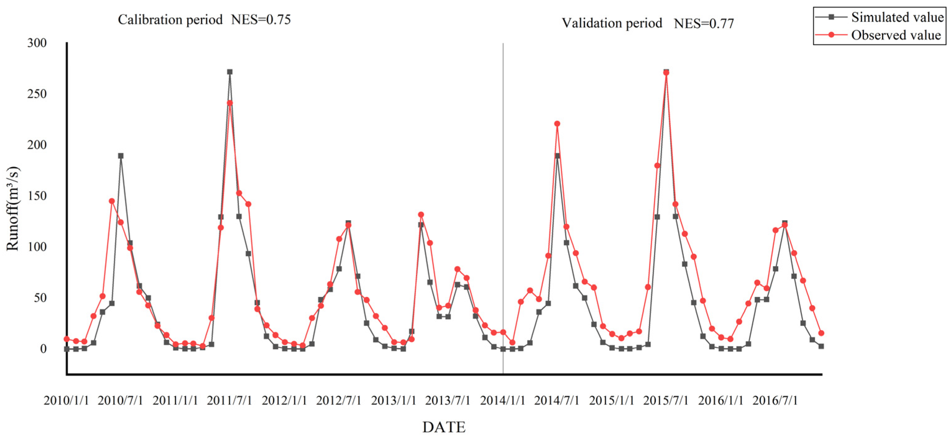
3.4.2. SWAT Model Evaluation

In this study, the determination coefficient (R²) [41] and the efficiency coefficient (NES) [42] are used to evaluate the model for its accuracy and reliability.

The determination coefficient (R²) represents the trend of change in difference between the simulation and measurement results of the model. The calculation formula is expressed as follows:

$${\mathrm{R}}^2=[\frac{\sum (\mathrm{M}-\overline{\mathrm{M}})(\mathrm{S}-\overline{\mathrm{S}})}{\sqrt{\sum (\mathrm{M}-\overline{\mathrm{M}}{)}^2(\mathrm{S}-\overline{\mathrm{S}}{)}^2}}{]}^2$$

(12)

The Nash–Sutcliffe efficiency coefficient (NES) is an important indicator used to assess the overall performance of the model. The higher the NES value [43], the better the model performs in terms of fitting and reliability. The calculation method is expressed as follows:

$$\mathrm{N}\mathrm{E}\mathrm{S}=1-\frac{{\sum }_{\mathrm{i}=1}^{\mathrm{n}}(\mathrm{S}-\mathrm{M}{)}^2}{{\sum }_{\mathrm{i}=1}^{\mathrm{n}}(\mathrm{S}-\overline{\mathrm{M}}{)}^2}$$

(13)

where:

M represents the simulation result;

S represents the measurement result;

$\overline{\mathrm{M}}$ represents the mean of simulation result;

$\overline{\mathrm{S}}$ represents the mean of measurement results; and

n represents the measured number.

4. Results and Discussion

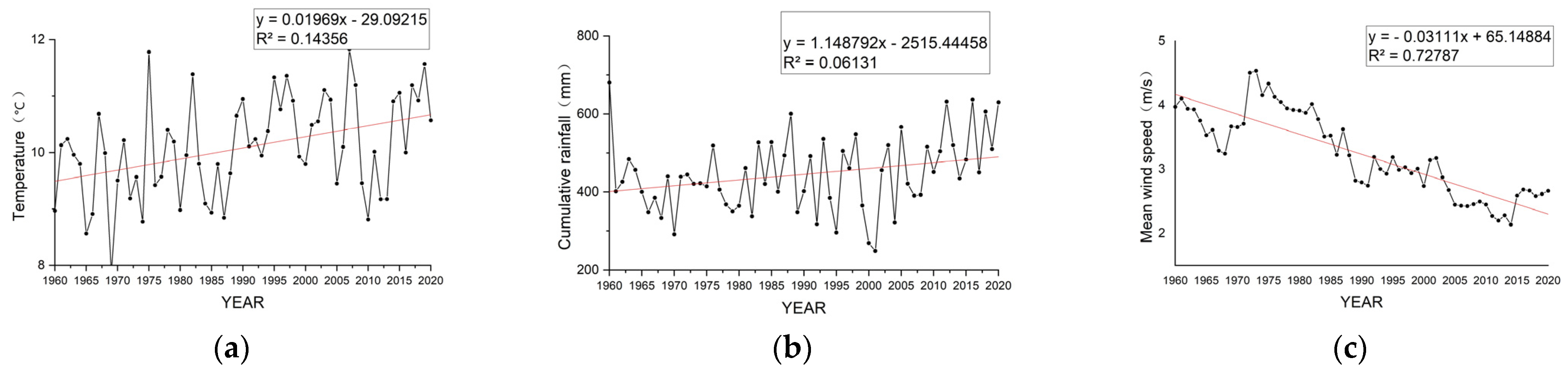
4.1. Characteristics of Climate Change in Hulan River Basin

According to the measurement data obtained from Wangkui Meteorological Station during the period between 1960 and 2020, Origin software(version 9.6.5.169) which was developed by OriginLab(U.S.A) for scientific mapping and data analysis, is used to plot the trend of changes in precipitation, temperature and wind speed, as shown in Figure 5. In addition, the linear regression equation is calculated. In the past 60 years, the precipitation and temperature in the Hulan River Basin showed an increasing trend. To be specific, the accumulative precipitation increased by 228.2 mm, and the fluctuation was most significant between 1995 and 1995, rising from 296.1 mm to 566.2 mm. The temperature rose by 1.6 °C, and the average wind speed dropped by 1.313 m/s. As can be seen from

Table 5. Average temperature, wind speed and precipitation of Wangkui Meteorological Station in each decade.

Year	Mean Temperature (°C)	Mean Precipitation (mm)	Mean Wind Speed (m/s)
1960–1969	9.51	435.49	3.71
1970–1979	9.86	407.48	4.09
1980–1989	9.71	448.13	3.55
1990–1999	10.59	430.70	2.98
2000–2009	10.49	410.07	2.68
2010–2019	10.31	522.83	2.45

, the variation in average temperature over each decade is 0.35 °C, −0.15 °C, 0.88 °C, −0.1 °C and −0.18 °C. Relative to the average value of multiyear periods, the difference of precipitation in the 1970s, 1980s, 1990s, 2000s and 2010s is −2.801, 4.065, −1.743, −2.063 and 10.223, respectively. The variation in wind speed in each decade is 0.38 m/s, −0.54 m/s, −0.67 m/s, −0.0.3 m/s and −0.23 m/s, respectively. Statistically, temperature, precipitation and wind speed have changed significantly over the past 10 years, indicating drastic climate change and the intensification of global warming and humidification.

As shown in Figure 6, the precipitation in the Hulan River Basin shows an alternation between positive and negative, with a continuous negative anomaly observed during the 1965–1975 period, indicating low precipitation in the probable annual period. A continuous positive anomaly occurred during the 2015–2020 period, indicating likely abundant annual precipitation, with the cumulative anomaly shaped like a “W”. During the 1960–1980 and 1987–2001 periods, the annual precipitation showed a decreasing trend. During the 1981–1985 and 2005–2020 periods, the annual precipitation showed an increasing trend.

4.2. Analysis Method and Model Results

The SWAT model is applied to simulate runoff in the watershed for the 2010–2013 period and to verify it for the 2014–2016 period, as shown in Figure 7. Compared with the measured runoff data in the simulation year, the correlation coefficient of the model is R² = 0.8439, and the coefficient of efficiency determination is NES = 0.75, indicating that the model meets the criteria of evaluation. After parameter calibration and sensitivity analysis conducted by SWAT-CUP for the model, R² = 0.9352 and NES = 0.77 for the simulation period, both of which are improved, as shown in Figure 8. On the whole, the simulation result of the model is slightly exceeded by the observational result, despite remaining in the allowable range of errors, indicating that the applicability of the model in this basin meets the standard. It thus provides a practical reference for hydrological simulation analysis of the rivers in Heilongjiang Province and other high-latitude cold areas.

5. Conclusions

In the present study, the data of temperature, precipitation and wind speed collected at the Wangkui Meteorological Station as a long time series are analyzed to determine the overall trend of climate change occurring in the Hulan River Basin. The SWAT model is also applied to simulate runoff in Hulan River Basin. After the introduction of snowmelt parameters and the revision of parameters by SWAT-CUP, the simulation result of runoff is found to be consistent with the measurement result. It is evidenced that SWAT is applicable to the rivers in those high-latitude cold areas.

In addition, given the effect on the scale of runoff on the change of land use [44], temperature [45] and precipitation [46], it is necessary to further study the correlation between these influencing factors.

The focus of our future study is to set the gradient of temperature change using the global warming caused by the reference RCP scenario model (RCP4.5, RCP6.0, RCP8.5), set other factors in the weather generator of the SWAT model to remain unchanged, change the data on precipitation and temperature, set a variety of climate change scenarios and study the impact of climate change on runoff in this basin. A land use transfer matrix will also be constructed using the land use data of different periods, and the impact of different types of land change on runoff will be quantitatively analyzed.

References

1. Jiang, J.C.; Zhu, A.-X.; Qin, C.; Liu, J.; Chen, L.; Wu, H. Review on distributed hydrological modelling software systems. J. Prog. Geogr. 2014, 33, 1090–1100. [Google Scholar]
2. Elhag, M.; Psilovikos, A.; Manakos, I.; Perakis, K. Application of the Sebs Water Balance Model in Estimating Daily Evapotranspiration and Evaporative Fraction from Remote Sensing Data Over the Nile Delta. Water Resour. Manag. 2011, 25, 2731–2742. [Google Scholar] [CrossRef]
3. Charizopoulos, N.; Psilovikos, A. Hydrologic processes simulation using the conceptual model Zygos: The example of Xynias drained Lake catchment (central Greece). Environ. Earth Sci. 2016, 75, 777. [Google Scholar] [CrossRef]
4. Zhang, Y.H. Development of Study on Model-SWAT and Its Application. J. Prog. Geogr. 2005, 24, 123–132. [Google Scholar]
5. Xu, A.T.; Mu, Z.W. Construction of SWAT Model Database in the Upper River Basin. J. Technol. Econ. Chang. 2021, 5, 114–116. [Google Scholar]
6. Neitsch, S.L.; Arnold, J.G.; Kiniry, J.R. Soil and Water Assessment Tool Theoretical Documentation Version 2005; Texas Water Resources Institute: Temple, TX, USA, 2005. [Google Scholar]
7. Grusson, Y.; Sun, X.L.; Gascoin, S.; Sauvage, S.; Raghavan, S.; Anctil, F.; Sachez-Perez, J.M. Assessing the capability of the SWAT model to simulate snow, snow melt and stream flow dynamics over an alpine watershed. J. Hydrol. 2015, 531, 574–588. [Google Scholar] [CrossRef]
8. Yen, H.; Sharifi, A.; Kalin, L.; Mirhosseini, G.; Arnold, J.G. Assessment of model predictions and parameter transferability by alternative land use data on watershed modeling. J. Hydrol. 2015, 527, 458–470. [Google Scholar] [CrossRef]
9. Malago, A.; Efstathiou, D.; Bouraoui, F.; Nikolaidis, N.P.; Franchini, M.; Bidoglio, G.; Kritsotakis, M. Regional scale hydrologic modeling of a karst-dominant geomorphology: The case study of the Island of Crete. J. Hydrol. 2016, 540, 64–81. [Google Scholar] [CrossRef]
10. Zhang, A.J.; Zhang, C.; Fu, G.B.; Wang, B.D.; Bao, Z.X.; Zheng, H.X. Assessments of Impacts of Climate Change and Human Activities on Runoff with SWAT for the Huifa River Basin, Northeast China. J. Water Resour. Manag. 2012, 26, 2199–2217. [Google Scholar] [CrossRef]
11. Conan, C.; de Marsily, G.; Bouraoui, F.; Bidoglio, G. A long-term hydrological modelling of the Upper Guadiana river basin (Spain). J. Phys. Chem. Earth 2003, 28, 193–200. [Google Scholar] [CrossRef]
12. Bosch, D.D.; Arnold, J.G.; Volk, M.; Allen, P.M. Simulation of a Low-Gradient Coastal Plain Watershed Using the SWAT Landscape Model. J. Trans. ASABE 2010, 53, 1445–1456. [Google Scholar] [CrossRef]
13. Sun, R.; Zhang, X.Q. Progress in Application of Watershed Runoff Simulation Based on SWAT. J. Hydrol. 2010, 30, 28–32+47. [Google Scholar]
14. Zhang, R.F.; Wang, J.L.; Li, C.X. Research Progress and Application Prospect of the SWAT Model. J. Sci. Technol. Eng. 2014, 14, 137–142+149. [Google Scholar]
15. Wang, Z.G.; Liu, C.M.; Huang, Y.B. The Theory of SWAT Model and its Application in Heihe Basin. J. Prog. Geogr. 2003, 22, 79–87. [Google Scholar]
16. Wu, J.; Zheng, H.; Xi, Y. SWAT-Based Runoff Simulation and Runoff Responses to Climate Change in the Headwaters of the Yellow River, China. J. Atmos. 2019, 10, 509. [Google Scholar] [CrossRef] [Green Version]
17. Wei, H.B.; Zhang, Z.P.; Yang, J.P. Establishing method for soil database of SWAT model. J. Water Resour. Hydropower Eng. 2007, 38, 15–18. [Google Scholar]
18. Wan, H.; Dong, X.; Peng, T.; Liu, J.; Yu, D.; Bo, H.; Chen, L. Application of the SWAT Model into the Runoff Simulation Based on SUFI-2 Algorithm in the East Branch of Huangbai River Basin. J. China Rural Water Hydropower 2018, 12, 94–100. [Google Scholar]
19. Omani, N.; Srinivasan, R.; Karthikeyan, R.; Smith, P.K. Hydrological Modeling of Highly Glacierized Basins (Andes, Alps, and Central Asia). J. Water 2017, 9, 111. [Google Scholar] [CrossRef] [Green Version]
20. Majed, A.-Z.; Lubna Bani, H. Assessment of the SWAT model in simulating watersheds in arid regions: Case study of the Yarmouk River Basin (Jordan). J. Open Geosci. 2021, 13, 377–389. [Google Scholar] [CrossRef]
21. Bajracharya, A.R.; Bajracharya, S.R.; Shrestha, A.B.; Maharjan, S.B. Climate change impact assessment on the hydrological regime of the Kaligandaki Basin, Nepal. J. Sci. Total Environ. 2018, 625, 837–848. [Google Scholar] [CrossRef]
22. Githui, F.; Gitau, W.; Mutua, F.; Bauwens, W. Climate change impact on SWAT simulated streamflow in western Kenya. Int. J. Climatol. 2009, 29, 1823–1834. [Google Scholar] [CrossRef]
23. Lucas-Borja, M.E.; Carrà, B.G.; Nunes, J.P.; Bernard-Jannin, L.; Zema, D.A.; Zimbone, S.M. Impacts of land-use and climate changes on surface runoff in a tropical forest watershed (Brazil). Hydrol. Sci. J. 2020, 65, 1956–1973. [Google Scholar] [CrossRef]
24. Zhang, Y.; Su, F.; Hao, Z.; Xu, C.; Yu, Z.; Wang, L.; Tong, K. Impact of projected climate change on the hydrology in the headwaters of the Yellow River basin. Hydrol. Process. 2015, 29, 4379–4397. [Google Scholar] [CrossRef]
25. Xuan, W.; Xu, Y.-P.; Fu, Q.; Booij, M.J.; Zhang, X.; Pan, S. Hydrological responses to climate change in Yarlung Zangbo River basin, Southwest China. J. Hydrol. 2021, 597, 125761. [Google Scholar] [CrossRef]
26. Ouyang, W.; Hao, F.; Skidmore, A.K.; Toxopeus, A.G. Soil erosion and sediment yield and their relationships with vegetation cover in upper stream of the Yellow River. Sci. Total Environ. 2010, 409, 396–403. [Google Scholar] [CrossRef]
27. Han, S.; Zhao, Y. Analysis of Variation Trendand Mutation Characteristics of Natural Run off in the Upstream of the Hulanhe River Basin. J. Water Resour. Power 2020, 38, 46–50. [Google Scholar]
28. Hou, W.; Liao, X.Y.; Zhang, Y.; Xue, H.; Xu, L. Construction of Basic Database for SWAT Model of the Typical Small Watershed in Sanxia Reservoir Area. J. Tibet. Univ. 2015, 30, 118–124. [Google Scholar]
29. Douglas-Mankin, K.R.; Srinivasan, R.; Arnold, J.G. Soil and Water Assessment Tool (SWAT) Model: Current Developments And Applications. J. Transation ASABE 2010, 53, 1423–1431. [Google Scholar] [CrossRef]
30. Wang, D.C.; Lu, Y.D. Development of Soil Erosion Models Abroad. J. Sci. Soil Water Conserv. 2004, 35–40. [Google Scholar]
31. Tian, Y.; Xiao, G.R. Runoff Simulation for Aojiang River Basin Using SWAT Model Driven by China Meteorological Assimilation Driving Datasets. J. Chang. River Sci. Res. Inst. 2020, 37, 27–32. [Google Scholar]
32. Fuka, D.R.; MacAllister, C.A.; Degaetano, A.T.; Easton, Z.M. Using the Climate Forecast System Reanalysis Dataset to Improve Weather Input Data for Watershed Models. J. Hydrol. Process. 2015, 28, 5613–5623. [Google Scholar] [CrossRef]
33. Xu, H.; Xu, C.Y.; Chen, S.; Chen, H. Similarity and Difference of Global Reanalysis Datasets (WFD and APH RODITE) in Driving Lumped and Distributed Hydrological Models in a Humid Region of China. J. Hydrol. 2016, 542, 343–356. [Google Scholar] [CrossRef]
34. Meng, X.Y.; Wang, H.; Lei, X.H.; Cai, S. Simulation validation and analysis of the Hydrological components of Jing and Bo River Basin based on the SWAT model driven by CMADS. J. Acta Ecol. Sin. 2017, 37, 7114–7127. [Google Scholar]
35. Zhang, C.H.; Wang, B.L. Evaluation of Runoff Simulation Effects of the SWAT Model Driven by CMADS and Traditional Meteorological Station Data-Taking the Case Study in Kushui River Basin. J. China Rural Water Hydropower 2018, 52–57. [Google Scholar]
36. Basu, A.S.; Gill, L.W.; Pilla, F.; Basu, B. Assessment of Variations in Runoff Due to Landcover Changes Using the SWAT Model in an Urban River in Dublin, Ireland. Sustainability 2022, 14, 534. [Google Scholar] [CrossRef]
37. Wang, L.; Du, H.; Xie, J.Z. SWAT Based Runoff Simulation of Qingshui River Basin in Zhangjiakou City. J. Hydroecol. 2020, 41, 34–40. [Google Scholar]
38. Abbaspour, K.C. SWAT-CUP 2012: SWAT Calibration and Uncertainty Programs–A User Manual; Swiss Federal Institute of Aquatic Science and Technology: Dübendorf, Switzerland, 2014. [Google Scholar]
39. Bai, S.; Wang, L.; Shi, J.; Li, W. Runoff simulation for Kaidu river basin based on SWAT model. J. Arid Land Resour. Environ. 2013, 27, 79–84. [Google Scholar] [CrossRef]
40. Ci, Y.Z.; Li, H.Y.; Li, X.F. Method and Application of SWAT Model Parameter Calibration for Spatial Heterogeneity of Snowmelt Runoff in Cold Regions of Northeast China: A Case Study of Baishan Basin. J. Jilin Univ. (Earth Sci. Ed.) 2023, 53, 230–240. [Google Scholar]
41. Nash, J.E.; Sutcliffe, J.V. River Flow Forecasting through Conceptual Model. Part 1—A Discussion of Principles. J. Hydrol. 1970, 10, 282–290. [Google Scholar] [CrossRef]
42. Legates, D.R.; McCabe, G.J. Evaluating the use of “goodness-of-fit” measures in hydrologic and hydroclimatic model validation. J. Water Resour. Res. 1999, 35, 233–241. [Google Scholar] [CrossRef]
43. Moriasi, D.N.; Arnold, J.G.; Van Liew, M.W.; Bingner, R.L.; Harmel, R.D.; Veith, T.L. Model evaluation guidelines for systematic quantification of accuracy in watershed simulations. J. Trans. ASABE 2007, 50, 885–900. [Google Scholar] [CrossRef]
44. Guzha, A.C.; Rufino, M.C.; Okoth, S.; Jacobs, S.; Nobrega, R.L.B. Impacts of land use and land cover change on surface runoff, discharge and low flows: Evidence from East Africa. J. Hydrol. 2018, 15, 49–67. [Google Scholar] [CrossRef]
45. Gosling, S.N.; Taylor, R.G.; Arnell, N.W.; Todd, M.C. A comparative analysis of projected impacts of climate change on river runoff from global and catchment-scale hydrological models. Hydrol. Earth Syst. Sci. 2011, 15, 279–294. [Google Scholar] [CrossRef] [Green Version]
46. Koukouli, P.G.; Georgiou, P.E.; Karpouzos, D.K. Assessing the Hydrological Effect of Climate Change on Water Balance of a River Basin in Northern Greece. Int. J. Agric. Environ. Inf. Syst. 2018, 9, 14–33. [Google Scholar] [CrossRef]
Figure 1. The basin.
Water 15 02845 g001
Figure 2. Land use map of Hulan River Basin in 2015.
Water 15 02845 g002
Figure 3. Soil types of Hulan River.
Water 15 02845 g003
Figure 4. SPAW operation interface.
Water 15 02845 g004
Figure 5. (a) Time series of mean temperature, (b) cumulative precipitation and (c) average wind speed at Wangkui Meteorological Station.
Water 15 02845 g005
Figure 6. (a) Precipitation anomaly from 1960 to 2020 in Hulan River Basin. (b) Cumulative anomaly from 1960 to 2020 in Hulan River Basin.
Water 15 02845 g006
Figure 7. A comparison between the simulation and measurement results of monthly runoff.
Water 15 02845 g007
Figure 8. A comparison of correlation coefficients between the calibration period (a) and the validation period (b).
Water 15 02845 g008