1. Introduction
Water hammer often occurs in various water pipe systems, including long-distance water transfer projects and hydropower stations. An abnormal pressure surge may lead to a pipe burst, so many water hammer protection measures are introduced to reduce the water hammer intensity. The air cushion surge chamber is a closed chamber that is partially filled with water and compressed air [
1]. As compared to an open-type pressure regulating chamber, it is rarely restricted by geological or topographical features, and offers numerous advantages, such as shorter construction supply, lower excavation volume, cost-effectiveness, and minimal ecological impact [
2]. The air cushion surge chamber is widely used in hydroelectric power plants for water hammer protection, ensuring the safe hydraulic operation of the water pipe system. In order to realize the safe and stable operation of water systems and the realization of intelligent operations, it is extremely important to accurately simulate the transient flow of pipe systems with an air cushion surge chamber.
The Method of Characteristics (MOC) is currently a widely used simulation tool for modeling the hydraulic transition process of hydroelectric power plants. However, there are some complicated situations, such as short pipes, T-junctions, and series pipes, in actual water delivery systems. When using MOC, interpolation or wave speed regulation is required, which reduces computational efficiency and accuracy and introduces computational errors. Moreover, most existing water hammer calculation models only adopt a steady friction model, implying that the friction inside the pipeline remains the same as the steady-state during the transient process. However, in actual transient processes, the friction inside the pipeline is influenced by multiple factors, leading to significantly different calculation results from the actual results. Additionally, they cannot accurately describe the waveform distortion and peak attenuation of pressure waves [
3].
The FVM discretized the calculation area in the pipeline into independent control units, and solved the differential equations in each unit separately. Godunov et al. [
4] proposed a numerical scheme for solving nonlinear Riemannian problems. This scheme is very suitable for approximating smooth solutions and discontinuous solutions. Therefore, in recent years, a large number of researchers have gradually begun to construct the Godunov scheme to solve the hydraulic transient water hammer problem.
Yazdi et al. [
5] pointed out in 2007 that when calculating hydraulic transients, if the Courant number condition is not met, the second-order Godunov scheme is more stable than the MOC method. Bi Sheng et al. [
6] adopted the Godunov scheme to solve the two-dimensional flow-transport equation. This model can simultaneously solve the water flux and transport flux, which is highly efficient for simulating the dynamic characteristics of water flow in complex terrain, and effectively eliminates problems such as excessive numerical damping and unstable oscillation caused by the convection term in numerical calculation. Zheng Jieheng et al. [
7] used the Godunov scheme to study the hydraulic transients in sequential transmission pipelines. Based on the finite volume method, Zhao Yue et al. [
8] proposed a treatment method with double virtual boundary to numerically simulate the phenomenon of water hammer and water column separation in pipelines. Zhou et al. [
9,
10,
11] proposed a method to simulate a liquid column separation-bridging water hammer using a second-order GODUNOV scheme. Hu et al. [
12] proposed the application of a second-order GODUNOV scheme to simulate non-pressurized flow.
Currently, there are two main unsteady friction models extensively utilized. These models are the weighted function model represented by the Zielke [
13] and the empirical correction model represented by the Brunone [
14]. According to the Zielke unsteady friction model, the instantaneous shear stress in the pipe due to transient flow is composed of a constant term and an additional term. The additional term uses the weighted function to account for the impact of historical velocity and acceleration on the current flow state. However, this method has a long calculation time and requires a large storage space. Subsequently, Zielke’s model was simplified by Trikha [
15], Vardy [
16], and other scholars, resulting in a weighted function class unsteady friction model with higher computational efficiency. The Brunone unsteady friction model links unsteady friction with instantaneous local acceleration and convective acceleration and proposes a new dynamic friction model. Vitkovsky [
17] improved the Brunone model by predicting the direction of water flow and wave propagation, as well as the effects of specific acceleration and deceleration stages.
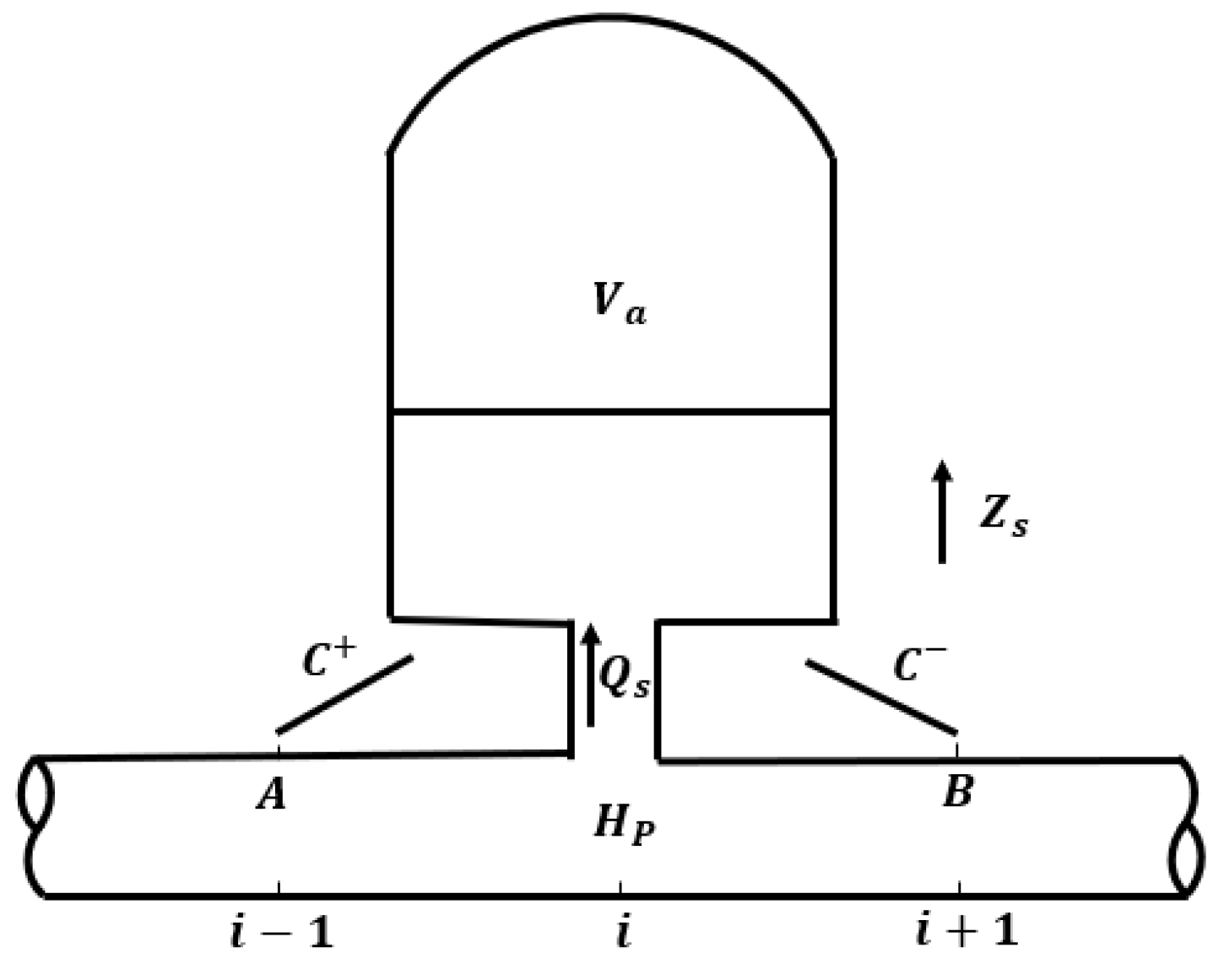
To simulate more accurately the hydraulic transient process of the pressurized delivery pipeline system with an air cushion surge chamber, this paper introduces the second-order Godunov format of FVM during the calculation process, incorporating the Trikha–Vardy–Brunone (TVB) and Brunone unsteady friction models. One virtual boundary method was proposed to realize the FVM simulation of an air cushion surge chamber. An experimental pipe system was designed and conducted to validate the proposed models in simulating the water hammer and dynamic behavior of an air cushion surge chamber.
The novelty of the paper is that a second-order FVM considering the effect of unsteady friction factor is developed to simulate the dynamic behavior of the air cushion surge chamber in a water pipeline system, while an experimental pipe system is conducted to validate the proposed numerical model. Pressure damping and energy dissipation of transient flow in a water pipeline system with air cushion surge chamber are carefully investigated and modeled, which have not been well considered in previous work.
4. Results and Discussion
4.1. Experimental Setup
An experimental pipe system was designed and conducted to validate the proposed models in simulating the water hammer and dynamic behavior of the air cushion surge chamber.
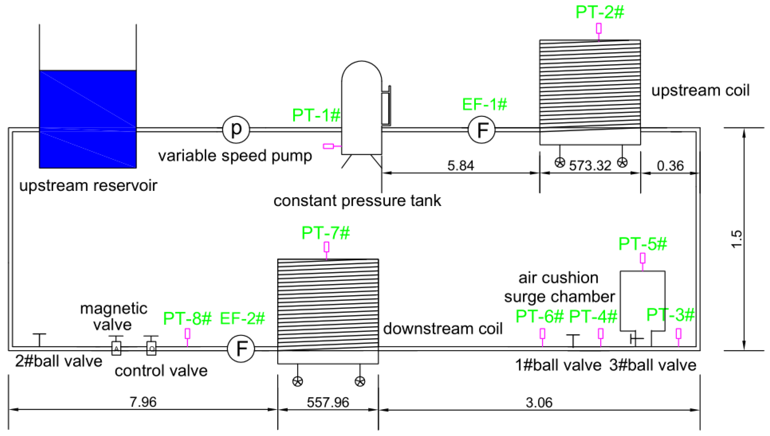
Figure 3 displays the experimental setup. The system consists of an upstream reservoir, variable frequency pump, constant pressure tank, upstream pipe, upstream electromagnetic flowmeter, and 1# ball valve. After the 1# ball valve, the pipeline serves as a return pipe. The water hammer experimental pipeline is 582 m long and is made of copper tubes, which have a wall thickness of 2 mm and an inner diameter of 21 mm. Along the pipeline, one 1/4 ball valve (1# ball valve) is arranged at the end, which is 582 m away from the upstream constant pressure tank. Additionally, five pressure sensors have been installed on the pipeline, with PT-1# measuring the pressure at the bottom of the constant pressure tank, PT-2# measuring 270 m downstream, PT-3# measuring 581.22 m downstream, PT-4# measuring 581.82 m downstream of the constant pressure tank, and PT-5# installed on the top of the air cushion surge chamber and used to measure the pressure of the gas in the gas chamber.
4.2. Water Hammer Problem in a Simple Reservoir–Pipe–Valve System
Four experimental conditions were conducted. The relevant parameters are shown in
Table 1.
H0 is constant pressure head in the upstream pressure tank.
Cases 1 and 2 exhibit laminar flow with Re = 1284, while cases 3 and 4 demonstrate low Reynolds number turbulence with Re = 4334.
The wave velocity of the water hammer in this experiment is calculated according to the experimental data measured by the pressure sensor. According to the pressure experimental data, the time difference between any two adjacent wave peaks is recorded as 2T, and then, according to the pipeline length L, water hammer wave a = 2L/T can be obtained. In addition, many factors can affect the water hammer wave velocity. In order to eliminate the interference, repeated tests were carried out on different experimental conditions and many times. Finally, the average value of multiple tests was taken as the value of the water hammer wave velocity in the subsequent numerical simulation. The wave velocity of the water hammer measured by the experiment is between 1260 m/s and 1360 m/s. In the numerical simulations, the wave speed is a = 1290 m/s and the experimentally observed range of the average resistance coefficient for the pipeline system under stable flow conditions is 0.0312~0.0356. Valve closing times ranged between 0.012 s and 0.026 s. The experimental results show that the valve closing time is much less than half of the pressure fluctuation period. Therefore, it is believed that the valve is closed instantaneously.
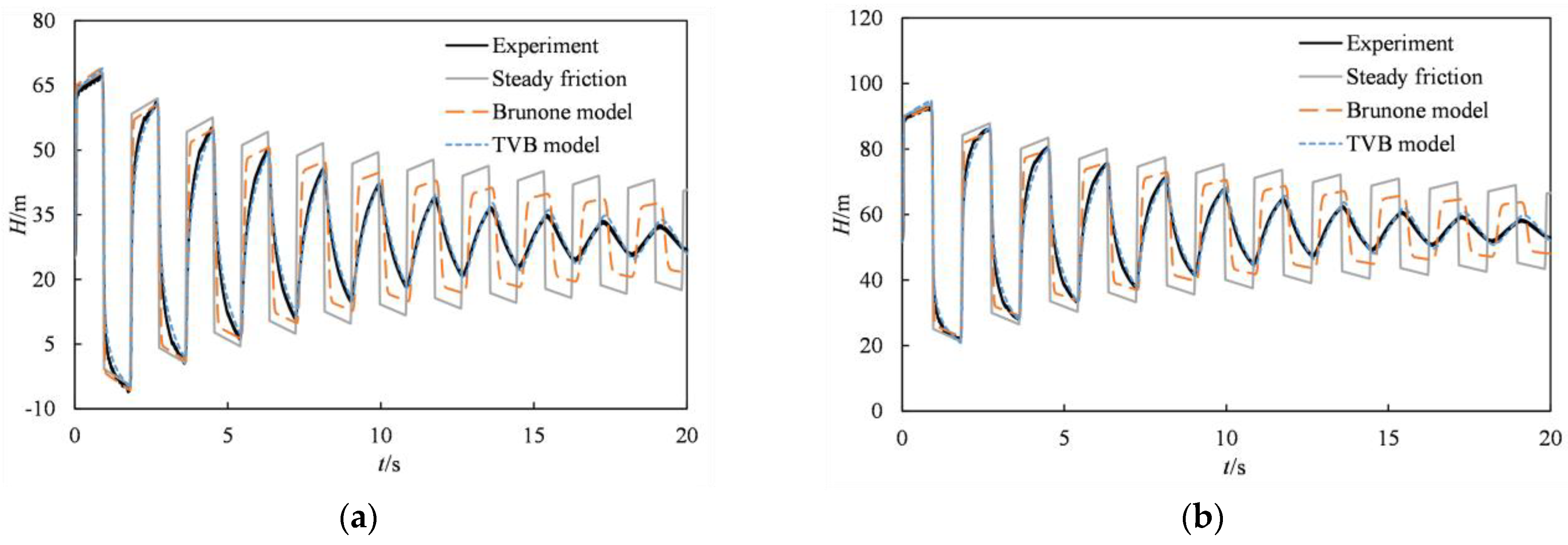
As shown in
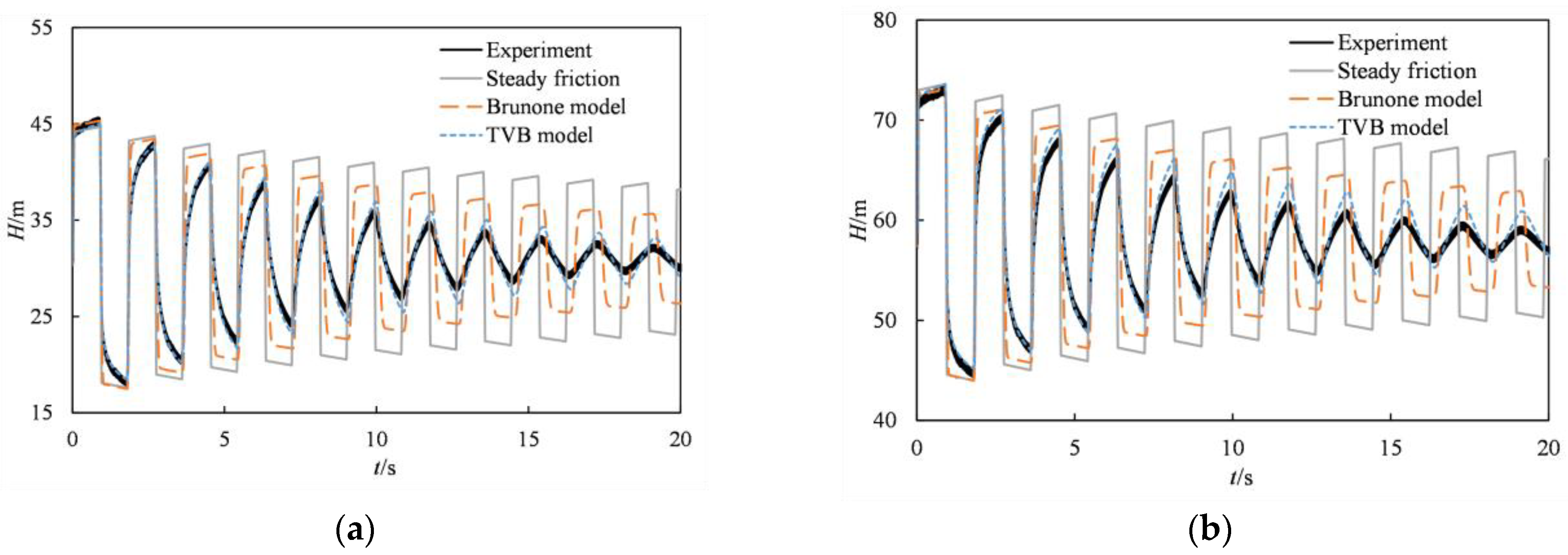
Figure 4, Cases 1 and 2 can produce a similar trend for experimental pressure oscillations, although with different reference values. This is because Cases 1 and 2 have the same Reynolds number Re = 1284, but different driving pressure heads (
H0 = 31 and 57). When the initial steady condition is under laminar flow in Case 1 and Case 2, the steady friction water hammer model can only accurately predict the first pressure peak, but fail to calculate well the subsequent pressure oscillations. The reason should be that, during the fast transient flow event, the pressure damping is mainly caused by the dynamic shear force near the pipe wall. However, the traditional water hammer model assumes that the dynamic shear force coefficient is constant. In order to verify this, the unsteady friction factor is considered in the water hammer events.
Figure 4a,b show that, compared to the steady friction water hammer model, the TVB and Brunone unsteady friction models can provide the much better simulation results. Meanwhile, it can be found that the TVB model shows the highest consistency with experimental results, while the Brunone unsteady friction model still produces the differences in simulating the later pressure peaks and the pressure oscillations. The main reason is that, as described above, the Brunone unsteady friction model is an empirically modified model, and the TVB model is a mechanism model which is derived from the physical equations.
Figure 5 shows the calculated and experimental results under the turbulence flow condition in Case 3 and Case 4. Cases 3 and 4 still produce a similar trend for experimental pressure oscillations, although with reference values. Similar to laminar flow cases, the comparisons still demonstrate that, under turbulence flow condition, the steady friction model can accurately predict only the first pressure peak, and significantly underestimates the pressure damping in the later pressure oscillations. In contrast to the steady friction model, the TVB and Brunone unsteady friction models can accurately predict the entire pressure attenuation process. Among these models, the TVB model can most accurately reproduce the experimental results.
It can also be found from
Figure 4 and
Figure 5 that, as the Reynolds number increases, the steady friction water hammer model can give better simulation results.
Overall, the TVB model can accurately reproduce the experimental results, regardless of the presence of laminar or turbulent flow, and is recommended to simulate the water hammer events.
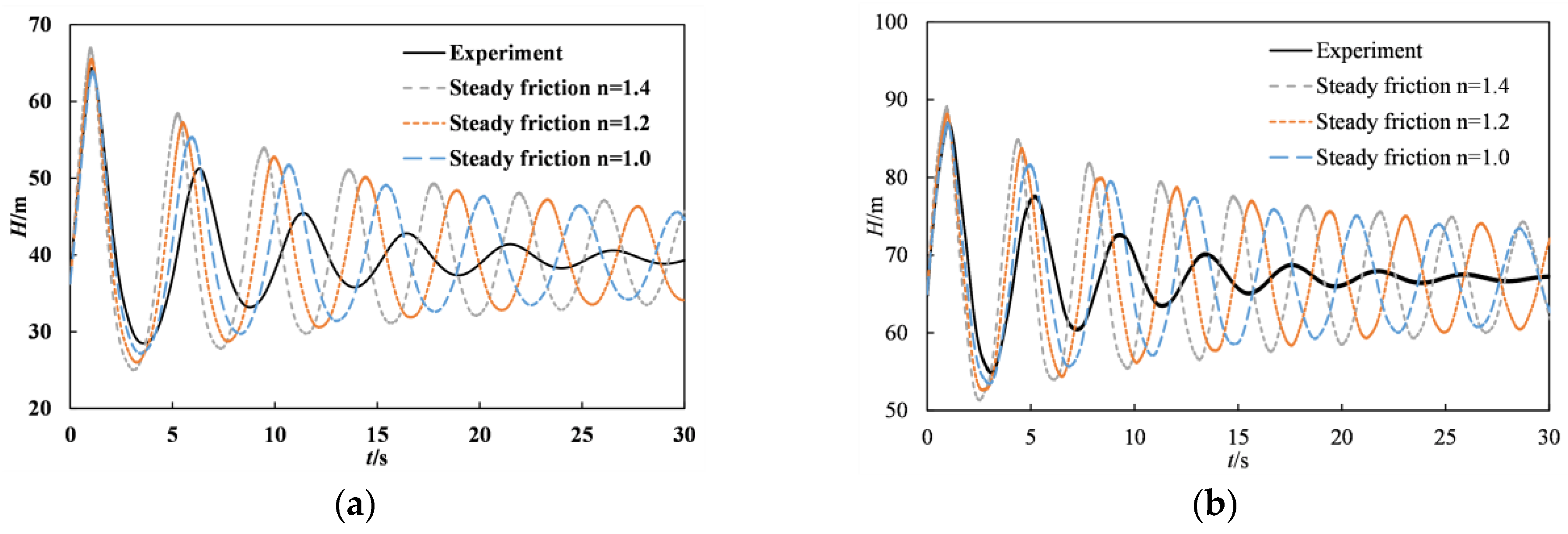
4.3. Water Hammer Problem with Air Cushion Surge Chamber
Figure 1 demonstrates that, by opening ball valve #3 on the connection pipe of the air cushion surge chamber, the experimental device transforms into a pressurized pipeline water supply system equipped with an air cushion surge chamber. Furthermore, a pressure sensor PT-5# is placed on top of the air cushion chamber to monitor the gaseous pressure inside it, and the steady-state gas pressure of the cushion surge chamber is also measured by this pressure sensor. The velocity of pressure wave in the air cushion surge chamber experiment is consistent with that of the above water hammer experiment without air cushion surge chamber, i.e., the wave speed is
a = 1290 m/s.
Table 2 presents the experimental conditions of the air cushion surge chamber.
The gas polytropic index,
n, is varied to 1.0, 1.2 and 1.4, where
n = 1.0 corresponds to an isothermal process,
n = 1.4 corresponds to an adiabatic process, and
n = 1.2 for the two in between, respectively, and the simulation results are depicted in
Figure 6.
Figure 6a,b display the results calculated by steady friction model and experimental results in Case 1 (laminar flow) and Case 3 (turbulent flow). Results show that a value of
n = 1.0 can simulate the pressure transient process of the gas in its first cycle more effectively than
n = 1.2 and
n = 1.4, although it still does not reproduce well the subsequent pressure oscillations.
Compared to
n = 1.2 and
n = 1.4, why is the result of
n = 1.0 closer to the experimental data? The main reasons are: (1) during the transient flow, air in the chamber experiences an expansion and deceleration process, which involves complicated heat transfer and thermodynamics; (2) in the existing numerical models, the air was assumed to follow the reversible polytropic relation [
18]; (3) the gas polytropic index,
n, is varied to 1.0, 1.2 and 1.4, where
n = 1.0 corresponds to an isothermal process,
n = 1.4 corresponds to an adiabatic process, and
n = 1.2 for middle process; (3) in this work, the heat transfer is serious, which makes the thermal process close to the isothermal process (
n = 1.0).
Meanwhile, why, even for
n = 1.0, do the calculated pressure oscillations attenuate lower than the measured ones? The reasons are that: (1) in the transient event in this work, the pressure damping (namely energy dissipation) is attributed to two aspects, in which one is energy loss due to heat transfer during air compression and expansion of air chamber, and another is hydraulic loss caused by the pipe friction; (2) results in
Figure 6 only consider the effect of the steady friction factor, neglecting the effect of unsteady friction.
Therefore, in the following section, the effect of unsteady friction will be included in the numerical simulation to enhance the numerical accuracy, as well as to verify the above explanation.
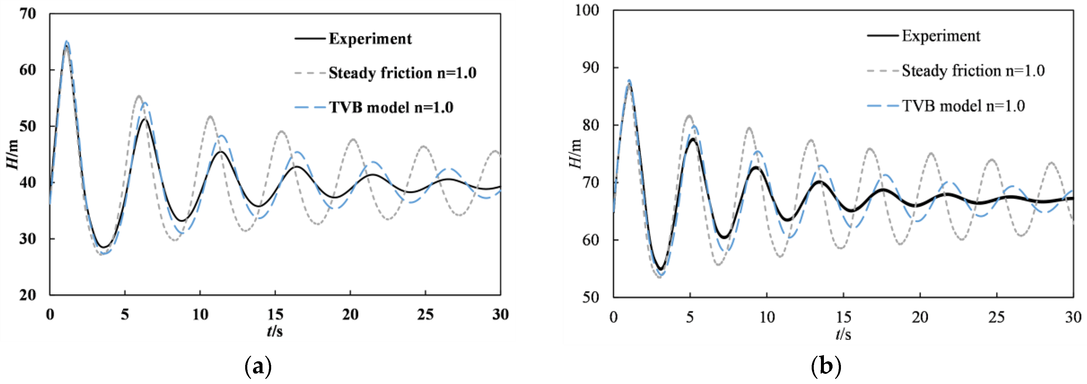
Figure 7 gives the results calculated by numerical models (steady and unsteady friction water hammer model) and experimental results in Case 1 (laminar flow) and Case 3 (turbulent flow). According to
Section 4.2, the TVB unsteady friction model performs better simulations for water hammer pressure of the pipeline in this experimental system. Therefore, the TVB unsteady friction model is adopted for this section. Additionally, examination of the simulation results from steady friction models indicated that
n = 1.0 provides the optimal simulation effect. Consequently, when using unsteady friction simulation,
n is set to 1.0.
As shown in
Figure 7, the results of Case 1 (laminar flow) and Case 3 (turbulent flow) both show that introduction of the unsteady friction model causes the first peak pressure to slightly increase, compared to the steady friction model. This is because air in the chamber experiences an expansion and deceleration process when the valve is quickly closed, and the unsteady friction model suppresses its deceleration, which results in the first pressure peak value increasing. However, in comparison to the steady friction model, the peak and cycle of the first period align more closely with experimental data. The peak value and cycle of the pressure decay process also exhibits better agreement with experimental data, indicating that the use of the unsteady friction model can more accurately simulate the hydraulic transient process of the pressurized pipeline water supply system. The difference between the peak pressure of the numerical simulation and the experimental results becomes larger, which is caused by the absence of wall heat exchange in the mathematical model. In future work, we will also take into account the energy loss caused by the heat exchange of the tube wall.
5. Conclusions
A second-order FVM considering the effect of unsteady friction factor is developed to simulate the water hammer and the dynamic behavior of air cushion surge chamber in a water pipeline system, while an experimental pipe system is conducted to validate the proposed numerical model. Two unsteady friction models, Brunone and TVB models, were incorporated into the water hammer equations, and the virtual boundary method was proposed to realize the FVM simulation of the air cushion surge chamber.
Comparisons with water hammer experimental results show that, while the steady friction model only accurately predicts the first pressure peak, it seriously underestimates pressure attenuation in later stages. Incorporating the unsteady friction factor can better predict the entire pressure attenuation process; in particular, the TVB unsteady friction model more accurately reproduces the pressure peaks and the whole pressure oscillation periods.
For water pipeline systems with an air cushion surge chamber, energy attenuation of the elastic pipe water hammer is primarily due to pipe friction and air cushion. The experimental results for the air cushion surge chamber demonstrate that the proposed FVM model with TVB unsteady friction model and the air chamber polytropic exponent near 1.0 can well reproduce the experimental pressure oscillations.
However, the difference between the peak pressures of the numerical simulation and the experimental results becomes larger, which is caused by the absence of wall heat exchange in the mathematical model. In the future, we will also take into account the energy loss caused by the heat exchange of the tube wall.


