
The Displacement of the Resident Wetting Fluid by the Invading Wetting Fluid in Porous Media Using Direct Numerical Simulation

Abstract
:1. Introduction
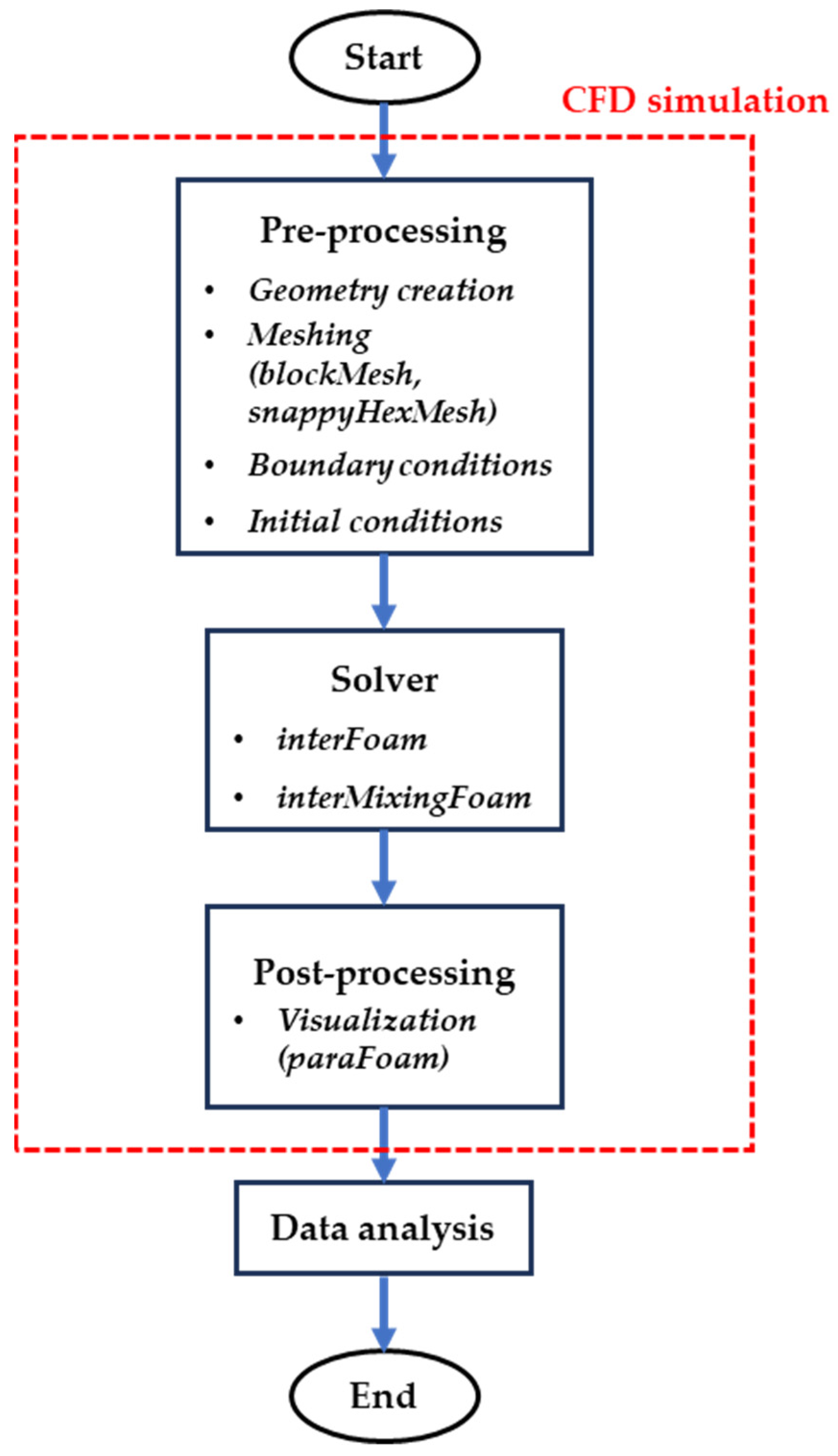
2. Methodology
2.1. Navier-Stokes Equations
2.2. Volume of Fluid (VOF) Method
2.3. Numerical Domain, Boundary, and Initial Conditions
2.4. Quantification of Fluid Saturations
3. Results and Discussions
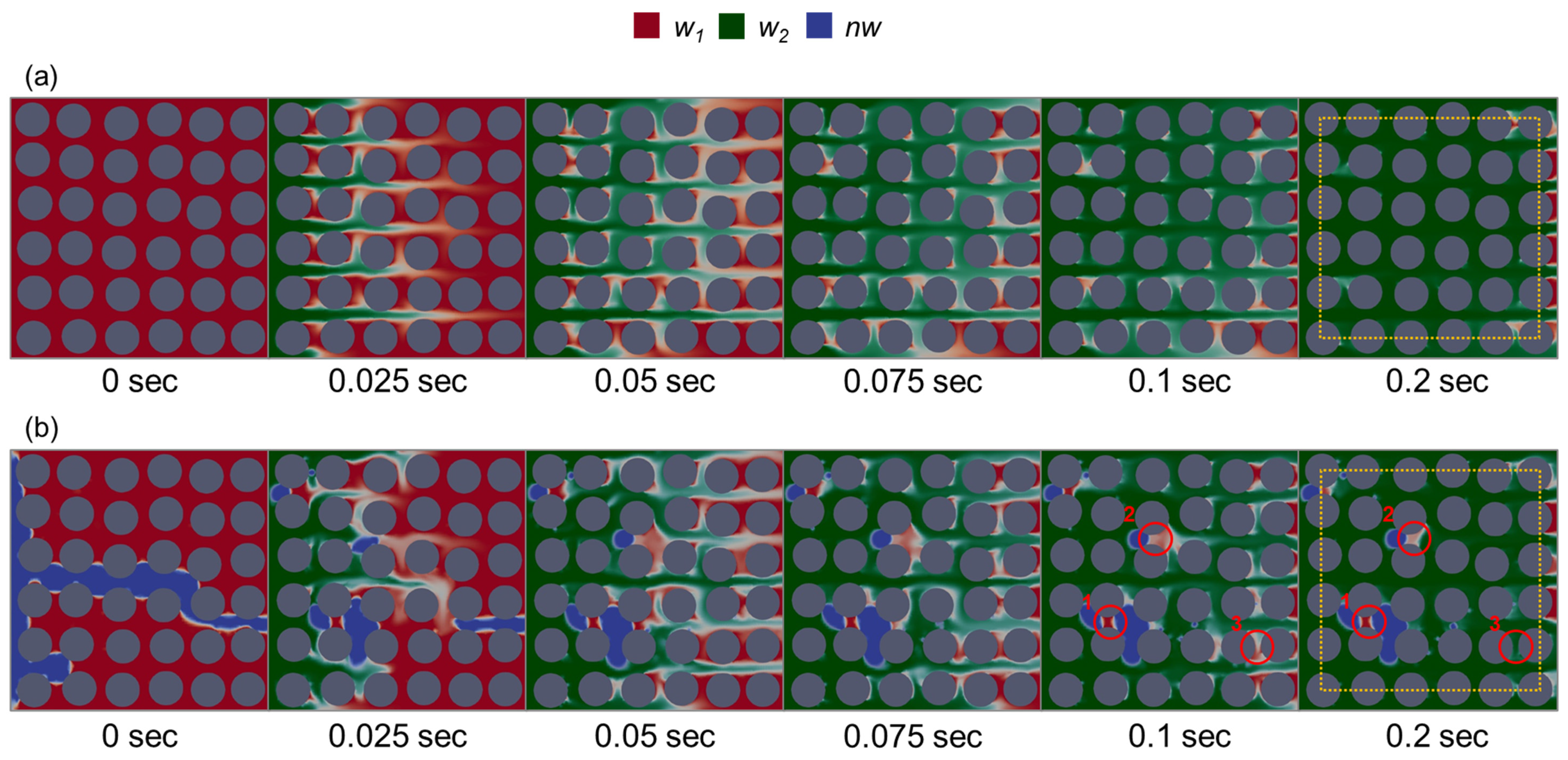
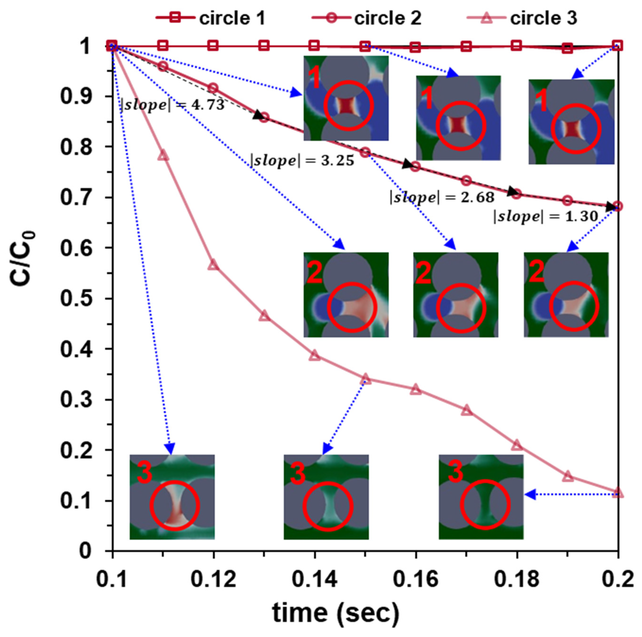
3.1. Effect of the Non-Wetting Phase (nw)
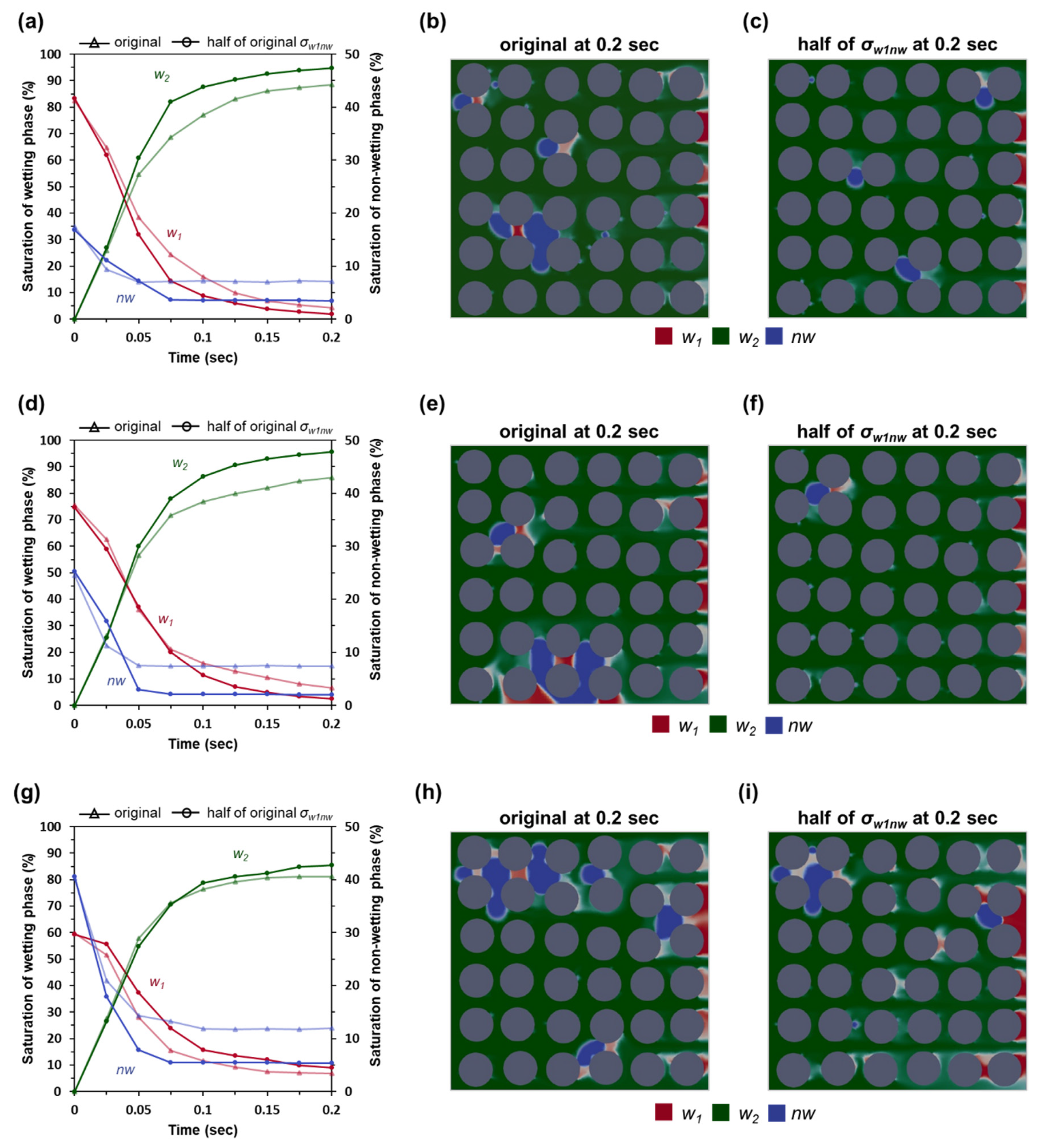
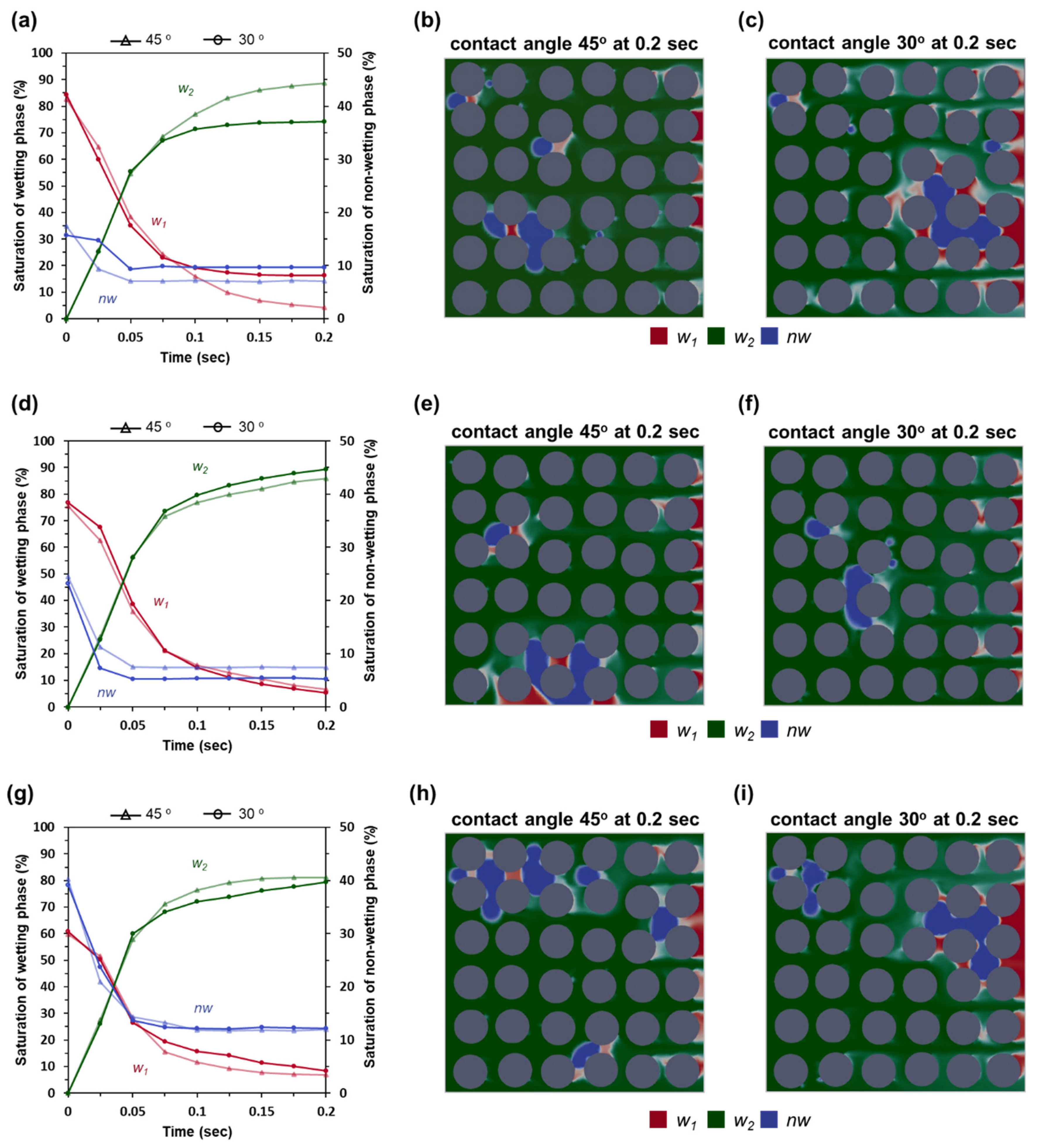
3.2. Effects of Interfacial Tension (σw1nw) and Contact Angle (θ)
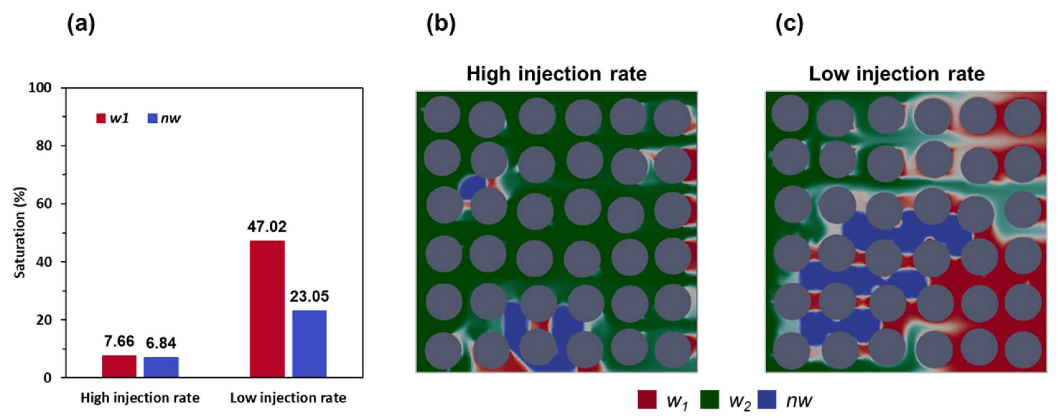
3.3. Effect of Injection Rate
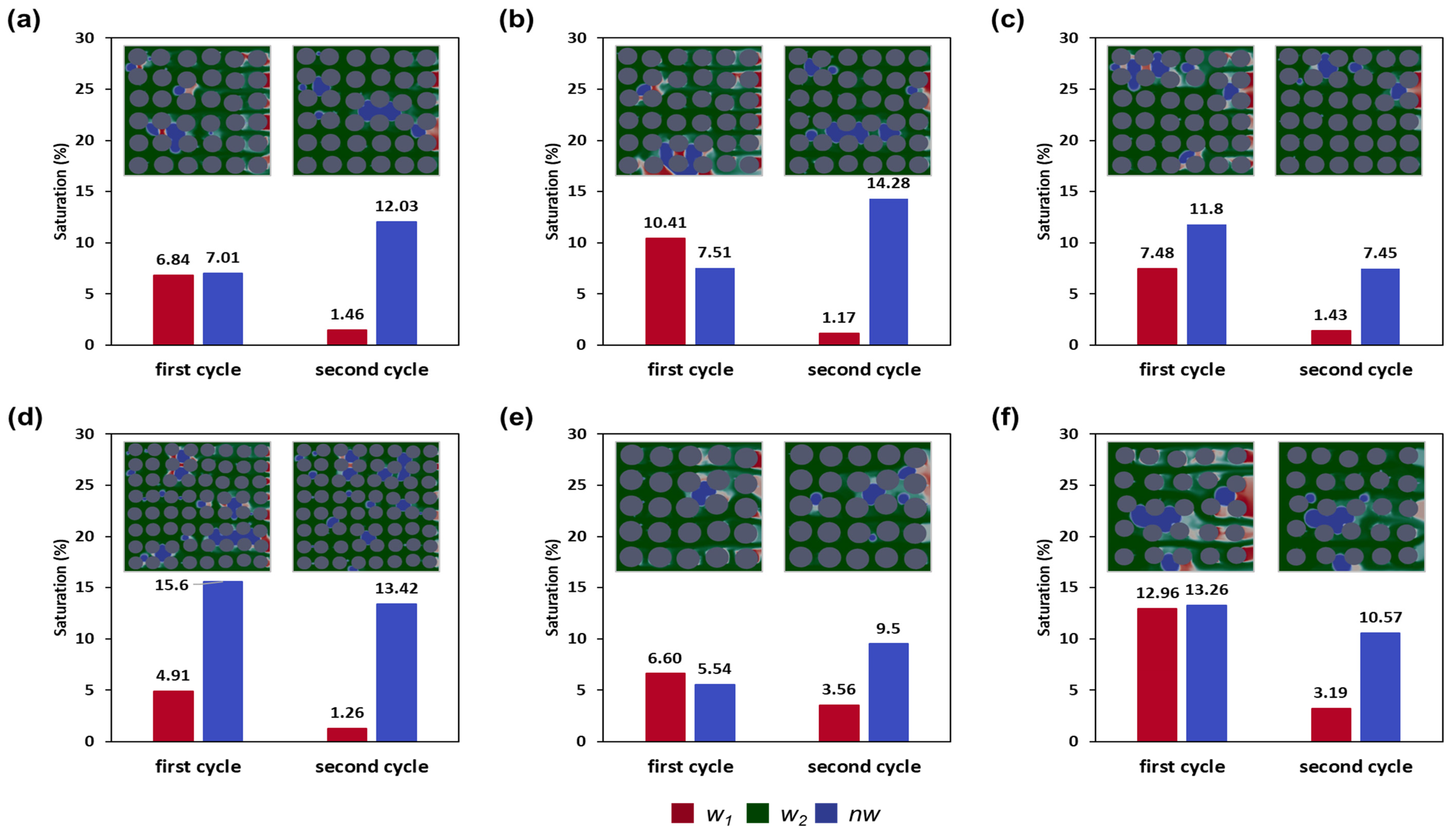
3.4. Effect of Drainage–Imbibition Cycles
3.5. Environmental Significance
4. Conclusions
- (1)
- When nw existed in the porous system, the displacement of w1 by w2 would be impeded. By calculating (C/C0) of w1 in the regions hindered by nw, it could be observed that w1 was displaced very slowly. This result helped explain the “slow-release phenomenon of old water” in previous column experiments.
- (2)
- When σw1nw decreased to half of the original value, the Sw1 would decrease because most of nw was flushed out. A change in contact angle (θ) caused a different distribution of nw in the system, which could result in a different displacement efficiency of w1.
- (3)
- At a very low injection rate = 0.01 m/s, w2 could not effectively displace w1 in porous media because of the remaining nw.
- (4)
- The drainage–imbibition cycles could improve the displacement of w1 in porous media because the constrained regions caused by nw were broken during consecutive drainage–imbibition cycles.
- (5)
- The simulation results have significantly advanced our understanding of future research and applications. In addition, the DNS method authentically described the immiscible fluid–fluid flow in porous media and could be easily applied to study physical mechanisms in other natural or industrial systems.
Author Contributions
Funding
Data Availability Statement
Acknowledgments
Conflicts of Interest
Appendix A


References
- Kim, K.Y.; Oh, J.; Han, W.S.; Park, K.G.; Shinn, Y.J.; Park, E. Two-phase flow visualization under reservoir conditions for highly heterogeneous conglomerate rock: A core-scale study for geologic carbon storage. Sci. Rep. 2018, 8, 4869. [Google Scholar] [CrossRef] [PubMed] [Green Version]
- Seyedpour, S.M.; Thom, A.; Ricken, T. Simulation of Contaminant Transport through the Vadose Zone: A Continuum Mechanical Approach within the Framework of the Extended Theory of Porous Media (eTPM). Water 2023, 15, 343. [Google Scholar] [CrossRef]
- Wang, L.; He, Y.; Wang, Q.; Liu, M.; Jin, X. Multiphase flow characteristics and EOR mechanism of immiscible CO2 water-alternating-gas injection after continuous CO2 injection: A micro-scale visual investigation. Fuel 2020, 282, 118689. [Google Scholar] [CrossRef]
- Wang, Y.; Fernàndez-Garcia, D.; Sole-Mari, G.; Rodríguez-Escales, P. Enhanced NAPL Removal and Mixing with Engineered Injection and Extraction. Water Resour. Res. 2022, 58, e2021WR031114. [Google Scholar] [CrossRef]
- Per- and Polyfluoroalkyl Substances (PFAS). Available online: https://www.epa.gov/pfas (accessed on 1 June 2023).
- Abraham, J.E.F.; Mumford, K.G.; Patch, D.J.; Weber, K.P. Retention of PFOS and PFOA Mixtures by Trapped Gas Bubbles in Porous Media. Environ. Sci. Technol. 2022, 56, 15489–15498. [Google Scholar] [CrossRef]
- Guo, B.; Zeng, J.; Brusseau, M.L. A Mathematical Model for the Release, Transport, and Retention of Per- and Polyfluoroalkyl Substances (PFAS) in the Vadose Zone. Water Resour. Res. 2020, 56, e2019WR026667. [Google Scholar] [CrossRef]
- Ji, Y.; Yan, N.; Brusseau, M.L.; Guo, B.; Zheng, X.; Dai, M.; Liu, H.; Li, X. Impact of a Hydrocarbon Surfactant on the Retention and Transport of Perfluorooctanoic Acid in Saturated and Unsaturated Porous Media. Environ. Sci. Technol. 2021, 55, 10480–10490. [Google Scholar] [CrossRef]
- Wang, Y.; Khan, N.; Huang, D.; Carroll, K.C.; Brusseau, M.L. Transport of PFOS in aquifer sediment: Transport behavior and a distributed-sorption model. Sci. Total Environ. 2021, 779, 146444. [Google Scholar] [CrossRef]
- Wang, Z.; Feyen, J.; van Genuchten, M.T.; Nielsen, D.R. Air entrapment effects on infiltration rate and flow instability. Water Resour. Res. 1998, 34, 213–222. [Google Scholar] [CrossRef]
- Wei, Y.; Chen, K.; Wu, J. Estimation of the Critical Infiltration Rate for Air Compression During Infiltration. Water Resour. Res. 2020, 56, e2019WR026410. [Google Scholar] [CrossRef]
- Gouet-Kaplan, M.; Berkowitz, B. Measurements of Interactions between Resident and Infiltrating Water in a Lattice Micromodel. Vadose Zone J. 2011, 10, 624–633. [Google Scholar] [CrossRef]
- Gouet-Kaplan, M.; Arye, G.; Berkowitz, B. Interplay between resident and infiltrating water: Estimates from transient water flow and solute transport. J. Hydrol. 2012, 458–459, 40–50. [Google Scholar] [CrossRef]
- Si, L.; Xi, Y.; Wei, J.; Wang, H.; Zhang, H.; Xu, G.; Liu, Y. The influence of inorganic salt on coal-water wetting angle and its mechanism on eliminating water blocking effect. J. Nat. Gas. Sci. Eng. 2022, 103, 104618. [Google Scholar] [CrossRef]
- Henry, E.J.; Smith, J.E. The effect of surface-active solutes on water flow and contaminant transport in variably saturated porous media with capillary fringe effects. J. Contam. Hydrol. 2002, 56, 247–270. [Google Scholar] [CrossRef]
- Li, Y.; Flores, G.; Xu, J.; Yue, W.Z.; Wang, Y.X.; Luan, T.G.; Gu, Q.B. Residual air saturation changes during consecutive drainage-imbibition cycles in an air-water fine sandy medium. J. Hydrol. 2013, 503, 77–88. [Google Scholar] [CrossRef]
- Tavangarrad, A.H.; Hassanizadeh, S.M.; Rosati, R.; Digirolamo, L.; van Genuchten, M.T. Capillary pressure–saturation curves of thin hydrophilic fibrous layers: Effects of overburden pressure, number of layers, and multiple imbibition–drainage cycles. Text. Res. J. 2019, 89, 4906–4915. [Google Scholar] [CrossRef] [Green Version]
- Gramling, C.M.; Harvey, C.F.; Meigs, L.C. Reactive Transport in Porous Media: A Comparison of Model Prediction with Laboratory Visualization. Environ. Sci. Technol. 2002, 36, 2508–2514. [Google Scholar] [CrossRef]
- Oates, P.M.; Harvey, C.F. A colorimetric reaction to quantify fluid mixing. Exp. Fluids. 2006, 41, 673–683. [Google Scholar] [CrossRef]
- De Anna, P.; Jimenez-Martinez, J.; Tabuteau, H.; Turuban, R.; Le Borgne, T.; Derrien, M.; Méheust, Y. Mixing and Reaction Kinetics in Porous Media: An Experimental Pore Scale Quantification. Environ. Sci. Technol. 2014, 48, 508–516. [Google Scholar] [CrossRef]
- Gouet-Kaplan, M.; Tartakovsky, A.; Berkowitz, B. Simulation of the interplay between resident and infiltrating water in partially saturated porous media. Water Resour. Res. 2009, 45, W05416. [Google Scholar] [CrossRef] [Green Version]
- Bandara, U.C.; Tartakovsky, A.M.; Palmer, B.J. Pore-scale study of capillary trapping mechanism during CO2 injection in geological formations. Int. J. Greenh. Gas. Control 2011, 5, 1566–1577. [Google Scholar] [CrossRef]
- Bandara, U.C.; Tartakovsky, A.M.; Oostrom, M.; Palmer, B.J.; Grate, J.; Zhang, C. Smoothed particle hydrodynamics pore-scale simulations of unstable immiscible flow in porous media. Adv. Water Resour. 2013, 62, 356–369. [Google Scholar] [CrossRef]
- Baakeem, S.S.; Bawazeer, S.A.; Mohamad, A.A. Comparison and evaluation of Shan–Chen model and most commonly used equations of state in multiphase lattice Boltzmann method. Int. J. Multiph. Flow. 2020, 128, 103290. [Google Scholar] [CrossRef]
- Li, P.; Berkowitz, B. Characterization of mixing and reaction between chemical species during cycles of drainage and imbibition in porous media. Adv. Water Resour. 2019, 130, 113–128. [Google Scholar] [CrossRef]
- Li, P.; Berkowitz, B. Controls on interactions between resident and infiltrating waters in porous media. Adv. Water Resour. 2018, 121, 304–315. [Google Scholar] [CrossRef]
- Ferrari, A.; Lunati, I. Direct numerical simulations of interface dynamics to link capillary pressure and total surface energy. Adv. Water Resour. 2013, 57, 19–31. [Google Scholar] [CrossRef]
- Ferrari, A.; Jimenez-Martinez, J.; Le Borgne, T.; Méheust, Y.; Lunati, I. Challenges in modeling unstable two-phase flow experiments in porous micromodels. Water Resour. Res. 2015, 51, 1381–1400. [Google Scholar] [CrossRef] [Green Version]
- Meakin, P.; Tartakovsky, A.M. Modeling and simulation of pore-scale multiphase fluid flow and reactive transport in fractured and porous media. Rev. Geophys. 2009, 47, RG3002. [Google Scholar] [CrossRef]
- OpenFOAM v9. Available online: https://openfoam.org/version/9/ (accessed on 1 June 2023).
- Hirt, C.W.; Nichols, B.D. Volume of fluid (VOF) method for the dynamics of free boundaries. J. Comput. Phys. 1981, 39, 201–225. [Google Scholar] [CrossRef]
- Ambekar, A.S.; Mattey, P.; Buwa, V.V. Pore-resolved two-phase flow in a pseudo-3D porous medium: Measurements and volume-of-fluid simulations. Chem. Eng. Sci. 2021, 230, 116128. [Google Scholar] [CrossRef]
- Aziz, R.; Joekar-Niasar, V.; Martinez-Ferrer, P. Pore-scale insights into transport and mixing in steady-state two-phase flow in porous media. Int. J. Multiph. Flow. 2018, 109, 51–62. [Google Scholar] [CrossRef] [Green Version]
- Deshpande, S.S.; Anumolu, L.; Trujillo, M.F. Evaluating the performance of the two-phase flow solver interFoam. Comput. Sci. Discov. 2012, 5, 014016. [Google Scholar] [CrossRef]
- Ziegler, A.; Bock, C.; Ketten, D.R.; Mair, R.W.; Mueller, S.; Nagelmann, N.; Pracht, E.D.; Schröder, L. Digital Three-Dimensional Imaging Techniques Provide New Analytical Pathways for Malacological Research. Am. Malacol. Bull. 2018, 36, 248–273. [Google Scholar] [CrossRef] [Green Version]


| Parameter | Value | Unit |
|---|---|---|
| density, ρw1 | 1000 | kg/m3 |
| density, ρw2 | 1000 | kg/m3 |
| density, ρnw | 1 | kg/m3 |
| kinetic viscosity, νw1 | 10−6 | m2/s |
| kinetic viscosity, νw2 | 10−6 | m2/s |
| kinetic viscosity, νnw | 1.48 × 10⁻⁵ | m2/s |
| interfacial tension, σw1nw | 0.0707 | kg/s2 |
| interfacial tension, σw2nw | 0.0707 | kg/s2 |
| Diffusivity, Dw1w2 | 3 × 10⁻⁹ | - |
| contact angle, θ | 45 | ° (degree) |
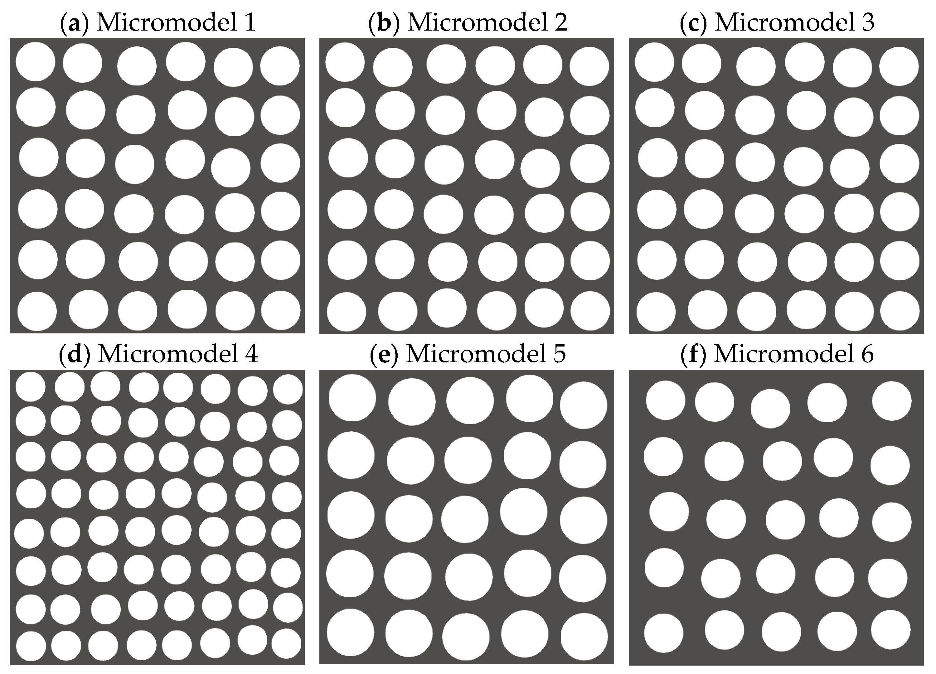
| Micromodel | Porosity (%) | Average Pore Radius (m) | Average Pore Throat (m) | Number of the Remaining nw Pockets | Final Image |
|---|---|---|---|---|---|
| Micromodel 1 | 49.73 | 3.53 × 10⁻⁴ | 2.39 × 10⁻⁴ | 4 |  |
| Micromodel 2 | 49.73 | 3.53 × 10⁻⁴ | 2.36 × 10⁻⁴ | 3 |  |
| Micromodel 3 | 49.73 | 3.53 × 10⁻⁴ | 2.38 × 10⁻⁴ | 6 |  |
| Micromodel 4 | 48.39 | 2.63 × 10⁻⁴ | 1.66 × 10⁻⁴ | 12 |  |
| Micromodel 5 | 49.73 | 4.41 × 10⁻⁴ | 2.73 × 10⁻⁴ | 1 |  |
| Micromodel 6 | 65.09 | 5.24 × 10⁻⁴ | 4.37 × 10⁻⁴ | 3 |  |
Disclaimer/Publisher’s Note: The statements, opinions and data contained in all publications are solely those of the individual author(s) and contributor(s) and not of MDPI and/or the editor(s). MDPI and/or the editor(s) disclaim responsibility for any injury to people or property resulting from any ideas, methods, instructions or products referred to in the content. |
© 2023 by the authors. Licensee MDPI, Basel, Switzerland. This article is an open access article distributed under the terms and conditions of the Creative Commons Attribution (CC BY) license (https://creativecommons.org/licenses/by/4.0/).
Share and Cite
Wang, Y.-L.; Huang, Q.-Z.; Hsu, S.-Y. The Displacement of the Resident Wetting Fluid by the Invading Wetting Fluid in Porous Media Using Direct Numerical Simulation. Water 2023, 15, 2636. https://doi.org/10.3390/w15142636
Wang Y-L, Huang Q-Z, Hsu S-Y. The Displacement of the Resident Wetting Fluid by the Invading Wetting Fluid in Porous Media Using Direct Numerical Simulation. Water. 2023; 15(14):2636. https://doi.org/10.3390/w15142636
Chicago/Turabian StyleWang, Yung-Li, Qun-Zhan Huang, and Shao-Yiu Hsu. 2023. "The Displacement of the Resident Wetting Fluid by the Invading Wetting Fluid in Porous Media Using Direct Numerical Simulation" Water 15, no. 14: 2636. https://doi.org/10.3390/w15142636