Article

Advancing Water Quality Research: K-Nearest Neighbor Coupled with the Improved Grey Wolf Optimizer Algorithm Model Unveils New Possibilities for Dry Residue Prediction

1
Laboratoire de Génie des Procédés Chimiques, Department of Process Engineering, University of Ferhat Abbas, Setif 19000, Algeria
2
Laboratory of Biomaterials and Transport Phenomena (LBMTP), University Yahia Fares, Medea 26000, Algeria
3
Faculty of Sciences, University of Medea, Nouveau Pole Urbain, Medea 26000, Algeria
4
Laboratory for Improvement of Phytosanitary Protection Techniques in Mountain Ecosystems (LATPPÉM), Department of Food Technology, University of Batna, Hadj Lakhdar, Biskra Avenue, Batna 05005, Algeria
5
Chemical Engineering Department, Process Engineering Faculty, University Constantine 3 Salah Boubnider, Constantine 25000, Algeria
6
Research Unit on Analysis and Technological Development in Environment (URADTE-CRAPC), BP 384, Bou-Ismail 42000, Tipaza, Algeria
7
Ecole Nationale Supérieure de Chimie de Rennes, CNRS, ISCR (Institut des Sciences Chimiques de Rennes)–UMR 6226, Univ Rennes, F-35000 Rennes, France
8
School of Engineering, Merz Court, Newcastle University, Newcastle upon Tyne NE1 7RU, UK
9
College of Engineering, Imam Mohammad Ibn Saud Islamic University, IMSIU, Riyadh 11432, Saudi Arabia
10
Laboratory of Management and Valorization of Natural Resources and Quality Assurance, SNVST Faculty, University of Bouira, Bouira 10000, Algeria
*
Author to whom correspondence should be addressed.
Water 2023, 15(14), 2631; https://doi.org/10.3390/w15142631
Submission received: 23 June 2023 / Revised: 14 July 2023 / Accepted: 18 July 2023 / Published: 20 July 2023
(This article belongs to the Special Issue Water Treatment Modeling and Nutrient Recovery Processes)

Abstract

:
Monitoring stations have been established to combat water pollution, improve the ecosystem, promote human health, and facilitate drinking water production. However, continuous and extensive monitoring of water is costly and time-consuming, resulting in limited datasets and hindering water management research. This study focuses on developing an optimized K-nearest neighbor (KNN) model using the improved grey wolf optimization (I-GWO) algorithm to predict dry residue quantities. The model incorporates 20 physical and chemical parameters derived from a dataset of 400 samples. Cross-validation is employed to assess model performance, optimize parameters, and mitigate the risk of overfitting. Four folds are created, and each fold is optimized using 11 distance metrics and their corresponding weighting functions to determine the best model configuration. Among the evaluated models, the Jaccard distance metric with inverse squared weighting function consistently demonstrates the best performance in terms of statistical errors and coefficients for each fold. By averaging predictions from the models in the four folds, an estimation of the overall model performance is obtained. The resulting model exhibits high efficiency, with remarkably low errors reflected in the values of R, R2, R2ADJ, RMSE, and EPM, which are reported as 0.9979, 0.9958, 0.9956, 41.2639, and 3.1061, respectively. This study reveals a compelling non-linear correlation between physico-chemical water attributes and the content of dry tailings, indicating the ability to accurately predict dry tailing quantities. By employing the proposed methodology to enhance water quality models, it becomes possible to overcome limitations in water quality management and significantly improve the precision of predictions regarding critical water parameters.

1. Introduction

Water is a vital resource essential for the survival and well-being of all living things on Earth [1]. It serves various purposes, including consumption, irrigation, power generation, temperature regulation, and industrial production [2]. Additionally, water plays a crucial role in the ecosystem, influencing climate, biodiversity, and biological cycles [3]. However, ensuring access to clean and safe water remains a significant challenge in many parts of the world, emphasizing the need for responsible water resource management [1]. To safeguard water quality, protect public health, and optimize water resource utilization, wastewater treatment plants play a crucial role [4,5]. These plants employ biological and physical processes to remove contaminants and waste from wastewater, including feces, chemicals, heavy metals, and sediment [6,7]. By treating wastewater, these plants contribute to preserving the water quality of rivers, lakes, and oceans, thus reducing the presence of harmful contaminants [5]. Moreover, they protect public health by preventing the contamination of drinking water sources and reducing the risks associated with harmful bacteria and other contaminants [5,7]. Furthermore, wastewater treatment plants safeguard the environment by preventing the pollution of soil and groundwater and the disruption of local flora and fauna [6]. They also enable efficient resource management by facilitating the reuse of treated water for purposes such as irrigation and energy production, alleviating the strain on drinking water supplies [8]. However, water treatment processes are not without drawbacks. They can be associated with high costs, substantial energy consumption, production of residues, limitations in treating certain contaminants, and challenges in their implementation for small communities [9]. Among these concerns, the management of dry residue, which refers to the solid substances remaining after water purification, is particularly important. Improper handling of dry residue, especially if it contains toxic substances like heavy metals or dangerous chemicals, can have adverse effects on human health and the environment. Discharged or stored dry residue has the potential to contaminate soils and groundwater and harm local flora and fauna, thus disrupting ecological balances. Furthermore, incorrect storage practices can pose safety hazards such as fires or leaks. Hence, it is crucial to manage dry residue correctly to preserve both human health and the environment. Nonetheless, continuous monitoring and sampling of large volumes of water over extended periods can be a costly and time-consuming endeavor [8]. Efforts are being made to develop more efficient and cost-effective monitoring techniques, including automated systems and remote sensing, to streamline water quality monitoring processes. To overcome these limitations, several scientific articles on using artificial intelligence (AI) in the field of water treatment have been published in recent years. A paper explores the use of bootstrap aggregate (DT_Bag) and least squares (DT_Lsboost) enhanced decision tree (DT) models to model organic matter in water as a function of physico-chemical parameters [6]. Another article investigated the prediction of sulfate levels in raw water using various machine learning models, including artificial neural networks (ANNs), support vector machines (SVMs), Gaussian process regression (GPR), DTs, and ensemble trees (ETs) [8]. Another article discusses the use of ANNs to predict the rate of soluble bicarbonate in drinking water in the Médéa region of Algeria [10]. Another paper describes a study that uses ANN and multiple linear regression (MLR) models to predict the soluble sulfate content in drinking water [11]. All of these papers have demonstrated that the introduction of AI in the field of water treatment can bring many benefits, such as improved efficiency, real-time monitoring, treatment customization, and prediction of potential problems [12]. The K-nearest neighbor (KNN) method is regarded as a cutting-edge approach for tackling complex modeling problems [13,14,15,16,17,18]. It involves utilizing sets of nearest neighbors for data processing and using pre-processed data to identify the closest neighbor match for the prediction process [18]. In addition, optimization algorithms like the improved grey wolf optimization (I-GWO) algorithm can also effectively evaluate the progression of the prediction process over time [18]. The I-GWO is a bio-inspired algorithm and can be used in conjunction with the KNN algorithm to categorize data [19]. By analyzing the data, the prediction process can be enhanced, enabling the validation of the properties measured during the optimization procedure [19].
This study introduces advancements in predicting dry residue content in water sources, addressing challenges associated with traditional monitoring methods. By establishing monitoring stations and utilizing the KNN model optimized by the improved grey wolf optimization (I-GWO) algorithm, the study significantly improves water quality management practices. The model incorporates 20 physical and chemical parameters as inputs, enabling a comprehensive understanding of factors influencing dry residue content. Rigorous optimization and cross-validation ensure accurate model configuration and performance assessment. The study highlights the non-linear correlation between water attributes and dry residue content, validating the accuracy and practical applicability of the model. This pioneering research enables the development of highly accurate and efficient water quality models, empowering informed decision-making for better water management practices. The novel combination of KNN and I-GWO provides a promising solution for predicting dry residues, opening new perspectives in water quality management. This innovative approach has implications for sustainable water resource management and environmental protection.
The remaining part of this article is organized as follows: The second section discusses the analysis of raw water and treated water from the Médéa region to establish the database, and the modeling of dry residues through the combined KNN and I-GWO (KKN_I-GWO) method. The third section provides an explanation of the developed model. Finally, the last section concludes the paper.

2. Materials and Methods

2.1. Database

The database used in this study consists of 400 samples of both raw and treated water collected from various locations in the Medea region throughout the year 2022. These samples were carefully chosen to cover a wide range of environmental conditions and potential sources of water contamination [20,21]. The samples were collected at regular intervals to capture seasonal variations and any temporal trends in water quality.
To ensure comprehensive analysis, a total of 21 physico-chemical parameters were measured in each water sample. These parameters were selected based on their known influence on water quality and their relevance to the study objectives. They encompassed a wide range of characteristics, including pH, conductivity, total dissolved solids, dissolved oxygen, temperature, and turbidity, as well as the concentrations of various ions, metals, organic compounds, and nutrients.
The analysis of the water samples and measurement of the physico-chemical parameters were performed following established protocols and guidelines. Specifically, the recommendations outlined in the 9th edition of the book Analyse de l’eau by Jean Rodier [22] were followed to ensure standardized and accurate measurements. These guidelines have been widely accepted in the field and provide reliable methods for assessing water quality.
For the database established, the input variables, which include the physico-chemical parameters, and the model output, dry residue, are given in Table 1 along with the statistical analysis (minimum “min”, mean, maximum “max” and standard deviations “STD” data).

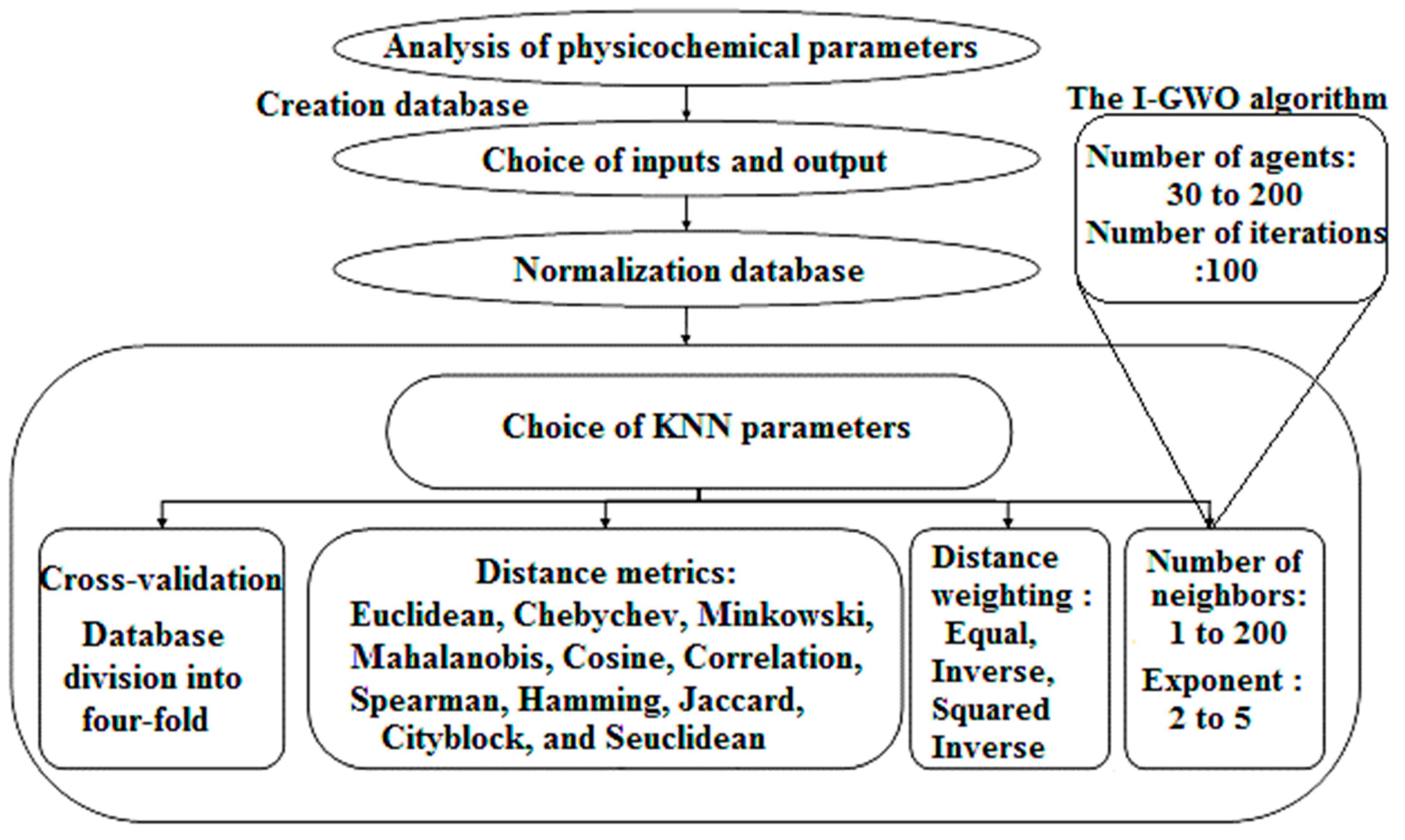
2.2. Modeling Method

The modeling method employed in this study is the KNN algorithm, a well-known and versatile machine learning technique. The KNN algorithm is particularly suitable for this study as it can handle both classification and regression tasks, making it ideal for predicting the dry residue in water based on the physico-chemical parameters [19,23].
In the KNN algorithm, the prediction for a given sample is based on the information from its k nearest neighbors in the feature space. The choice of the appropriate value for k depends on the specific characteristics of the dataset and the desired level of accuracy [19,23]. In this study, various values of k were considered and optimized using the improved grey wolf optimizer (I-GWO) algorithm, a metaheuristic optimization technique.
The I-GWO algorithm, an enhancement of the grey wolf optimizer, introduces several improvements to enhance its optimization capabilities [24,25]. These include a leader selection mechanism based on the standard deviation of wolf positions, an improved method for updating the wolf positions to prevent stagnation and facilitate convergence, as well as adaptive parameter management for improved robustness and stability [24,25].
To ensure reliable model performance and mitigate the risk of overfitting, a four-fold cross-validation approach was employed. The dataset was divided into four subsets, with three subsets used for training the KNN model and the remaining subset used for validation. This process was repeated four times, with each subset serving as the validation set once, resulting in a comprehensive assessment of the model’s generalization capabilities.
Furthermore, to optimize the KNN model’s parameters, an extensive search was conducted over a range of distance metrics, including Euclidean, Chebychev, Minkowski, Mahalanobis, Cosine, Correlation, Spearman, Hamming, Jaccard, Cityblock, and Seuclidean. Each distance metric was accompanied by its corresponding distance weighting functions, such as equal, inverse, and squared inverse. The parameters of each distance metric were fine-tuned using the I-GWO algorithm, optimizing factors such as the number of neighbors and the exponent for the Minkowski distance metric.
During the optimization process, careful consideration was given to the computational requirements and model performance. The number of neighbors ranged from 1 to 200, and the exponent for the Minkowski distance metric was explored within the range of 2 to 5. The I-GWO algorithm was configured with a maximum number of iterations of 100, and the number of agents, a parameter controlling the search space exploration, was optimized between 30 and 200.
By utilizing this comprehensive approach, involving cross-validation, parameter optimization, and the integration of KNN and I-GWO algorithms, we aimed to develop an accurate and reliable prediction model for estimating the dry residue in water based on the measured physico-chemical parameters.
A detailed design of the KNN_I-GWO model development method is presented in Figure 1.
In order to assess the performance of the models and select the optimal one, statistical measures were used. These measures included the correlation coefficient (R), coefficient of determination (R2), adjusted coefficient of determination (R2adj), root mean square error (RMSE), and Error Prediction of Model (EPM). The formulas used to calculate these criteria were as follows [26,27,28,29,30,31,32]:
R = i = 1 N ( y exp y ¯ exp ) ( y pred y ¯ pred ) i = 1 N ( y exp y ¯ exp ) 2 i = 1 N ( y pred y ¯ pred ) 2
R adj 2 = 1 ( 1 R 2 ) ( N 1 ) N K 1
RMSE = ( 1 N ) ( i = 1 N [ ( y exp y pred ) ] 2 )
EPM ( % ) = 100 N i = 1 N | ( y exp y pred ) y exp |
where N is the number of data samples; K is the number of variables (inputs); y exp and y pred are the experimental and the predicted values, respectively; and y ¯ exp and y ¯ pred are the average values of the experimental and the predicted values, respectively [33,34,35].

3. Results and Discussion

3.1. Factors Affecting Water Quality and Dry Residue

Water quality can be significantly influenced by numerous factors throughout the year, including precipitation, temperature, human activities, topography, and water management [20,21]. Intense precipitation events can lead to runoff and flooding, resulting in higher levels of turbidity and increased concentrations of contaminants such as sediments, nutrients, pesticides, and heavy metals. Additionally, warm temperatures create favorable conditions for the growth of algae and bacteria, which deplete dissolved oxygen in the water and harm aquatic organisms. Human activities, such as chemical and wastewater discharge, as well as agricultural, industrial, and residential practices, contribute to water pollution. Moreover, topography plays a crucial role, as steep slopes promote soil erosion and sediment accumulation, while low-lying areas are more prone to flooding and stagnant water. Practices associated with water management, including damming, reservoirs, and wastewater and drinking water treatment, also have a significant impact on water quality.
The dry residue of water refers to the amount of dissolved matter remaining after complete evaporation [36,37,38,39,40]. However, accurately predicting dry residues can be challenging due to various factors, such as the water source, water treatment methods, environmental conditions, and seasonal variations [36,37,38,39,40]. Therefore, considering these factors is essential when attempting to predict dry residues in water. Additionally, regular collection of water quality data is crucial to improve the accuracy of such predictions.
To address these concerns, water samples from different locations in the Medea region were collected throughout 2022. These samples underwent analysis using 21 physico-chemical parameters, following the recommendations outlined in the ninth edition of the book Analyse de l’eau by Jean Rodier [22].
The selection of these 21 physico-chemical parameters was based on several important considerations. Laboratory experience has shown that dry residue can contain a wide range of components, including minerals, salts, metals, non-volatile organic compounds, residues of chemical products, dissolved organic matter, and microorganisms [41,42,43].
The relationships between these physico-chemical parameters and the dry residue are often non-linear, as evidenced by various studies in the literature [6]. For instance, the presence of sulfate ions in water is associated with essential cations such as calcium, magnesium, and sodium [44]. Calcium, being a dominant element in drinking water, is primarily linked to the dissolution of carbonate formations or gypsum [45], while magnesium significantly contributes to water hardness, existing in similar forms to calcium [22]. The hardness of water, determined by the presence of calcium and magnesium salts, is directly influenced by the geological nature of the surrounding land [44]. Furthermore, the sum of cations is equal to the sum of anions due to ion balance considerations [6]. Considering the composition of the dry residue and the aforementioned relationships, it can be inferred that all 21 physico-chemical parameters have a non-linear influence on the dry residue, justifying their inclusion in the analysis. Due to the complex nature of the relationships among these parameters, their non-linear behavior, and their interdependence, conducting sensitivity analysis and significance testing was not necessary.
In the context of data-driven modeling, a larger database increases the likelihood of effectively covering the input and output space, thus representing various classes or categories of data in the training data. This improves the accuracy of predictions by enabling the KNN model to identify the k nearest neighbors that closely match the input datum [13,46,47]. Additionally, a larger database allows for a more accurate estimation of the probability density distribution of the data, facilitating better modeling of the relationships between different characteristics of the data. Furthermore, a larger dataset reduces the risk of overfitting the model to specific data [13,46,47]. However, it is important to strike a balance between the quantity of modeling data and the associated efforts required for data collection. Therefore, in this study, a total of 400 samples of raw and treated water were collected from different locations in the Medea region.

3.2. KNN Model

As previously mentioned, this research utilized the KNN model with cross-validation to assess predictive model performance, optimize model parameters, and reduce the risk of overfitting during model fitting. The dataset was split into four folds, with each fold serving once as the validation set and the other three folds forming the training set. The KNN_I-GWO model was then trained on the training set and evaluated on the validation set, with this process repeated four times. Model performance was assessed using various statistical measures, including R, R2, R2adj, RMSE, and EPM. The eleven distance metrics used in the KNN model (Euclidean, Chebychev, Minkowski, Mahalanobis, Cosine, Correlation, Spearman, Hamming, Jaccard, Cityblock, and Seuclidean) were optimized alongside their corresponding distance weighting functions (such as equal, inverse, and squared inverse) for each fold. The specific parameters of the metric distance checks, particularly the implementation of Minkowski distance metrics and the neighboring noble, were optimized using the I-GWO algorithm. It is important to note that the number of neighbors has been optimized in the range from 1 to 200, and for the Minkowski distance (cubic), the exponent has been optimized in the range from 2 to 5. For the I-GWO algorithm, the number of iterations was set to 100, while the number of agents was optimized in the range of 30 to 200.
Once the four optimal models were formed and tested, the prediction values produced by these four optimal models were aggregated to calculate the average of the predictions and obtain an estimate of the overall performance of the model.
Table 2 shows the performance of the best models obtained from the optimization of the 11 dissemination measures and their weighting functions. Table 2 shows the performance measures, R, R2, R2adj, RMSE, and EPM, for the best models on the training data, the validation data, and all data.
Table 2 presents the results of optimizing a KNN model using the I-GWO algorithm. The model was optimized by using different distances and distance weights, as well as varying the number of neighbors. The values of R, R2, R2adj, RMSE and EPM were calculated for each fold of the cross-validation and for the average of the folds for the training (Train), validation (VAL), and overall (ALL) data.
The best results were achieved through a systematic and rigorous approach that involved using a combination of distance and distance weighting for each ply in the model. This optimal combination was obtained using the Jaccard distance with an inverse squared distance weighting and with the number of iterations and the number of grey wolf agents at 100 and 50, respectively, for each fold. The best models were obtained for the number of neighbors ranging from three to seven (three neighbors for the first fold, five neighbors for the second fold, six neighbors for the third fold, and seven neighbors for the fourth fold). The values of R, R2, and R2adj for the training data are all very high for each fold, which indicates an excellent ability of each optimal model obtained to predict the dry residue values for the training data. The values of RMSE are also low in each fold, indicating that the predictions are on average very close to the true values, and the value of MAE was also low, indicating that the predictions are on average very accurate.
The values of R, R2, and R2adj for the validation data are also high in each fold, suggesting that the model has good predictive ability and explains much of the variance in the validation data. The RMSE and EPM values for the validation are higher than those for the training data, but still relatively low compared to the optimal experimental value of dry residue, 3000 mg/L.
In the first fold, utilizing three neighbors, the model demonstrated exceptional performance. For the training data, the R, R2, and R2adj values were 0.9958, 0.9916, and 0.9910, respectively. These high values indicate that the optimized model can explain a significant portion of the variance in the training data. The model also showed strong performance on the validation data, with R, R2, and R2adj values of 0.9951, 0.9902, and 0.9877, respectively. These results suggest that the model has good predictive ability and can generalize well to unseen data. The RMSE and EPM values for the training data were 56.0826 and 2.7224, indicating that, on average, the predictions were close to the true values with low error. The RMSE and EPM values for the validation data were 70.2751 and 3.2649, showing that the model’s predictions were slightly less accurate for the validation phase but still within an acceptable range. These values are relatively low compared to the optimal experimental value of dry residue, 3000 mg/L, indicating the model’s effectiveness in predicting dry residue values.
In the second fold, employing five neighbors, the model continued to exhibit strong performance. The R, R2, and R2adj values for the training data were 0.9948, 0.9896, and 0.9888, respectively. The values of R, R2, and R2adj showed similar high values on the validation data, with values of 0.9924, 0.9848, and 0.9809, respectively. The RMSE and EPM values for the training data were 65.8544 and 3.2718, and for the validation data, they were 79.3686 and 4.3136. These values indicate that the model’s predictions were slightly less accurate for the validation phase compared to the training phase, but still relatively low compared to the optimal experimental value of dry residue, 3000 mg/L.
In the third fold, utilizing six neighbors, the model once again delivered strong performance. The R, R2, and R2adj values for the training data were 0.9968, 0.9937, and 0.9932, respectively. For the validation data, the corresponding values were 0.9880, 0.9761, and 0.9700, suggesting that the model’s predictions explained a significant portion of the variance in the validation data. The RMSE and EPM values for the training data were 48.5324 and 2.2022, respectively, and for the validation data were 110.9024 and 5.1410, respectively. These values indicate that the model’s predictions were very close to the true values for the training phase, but slightly higher for the validation phase, while still relatively low compared to the optimal experimental value of dry residue, 3000 mg/L.
In the fourth fold, employing seven neighbors, the model continued to demonstrate strong performance. The R, R2, and R2adj values for the training data were 0.9930, 0.9861, and 0.9851, respectively. For the validation data, the corresponding values were 0.9948, 0.9897, and 0.9871, respectively, suggesting that the model’s predictions explained a significant portion of the variance in the validation data. The RMSE and EPM values for the training data were 75.7243 and 3.0832, and for the validation data, they were 63.0681 and 3.8588. These values confirm the model’s ability to provide accurate and consistent predictions, while still being relatively low compared to the optimal experimental value of dry residue, 3000 mg/L.
Considering all the folds, the average of the models yielded outstanding results. The average R, R2, and R2adj values were 0.9979, 0.9958, and 0.9956, respectively. The average RMSE and EPM values were 41.2639 and 3.1061, respectively, further indicating the model’s accuracy in predicting dry residue values with low error. These values are considerably lower than the optimal experimental value of dry residue, 3000 mg/L, emphasizing the model’s effectiveness in predicting dry residue values.
To evaluate the performance of the obtained KNN_I-GWO models, the average predictions of the models for all four folds were calculated in the cross-validation process, which resulted in a highly efficient model. This model showed high statistical coefficients (R = 0.9979, R2 = 0.9958, and R2adj = 0.9956) as well as low statistical errors (RMSE = 41.2639 and EPM = 3.1061), indicating a high level of precision in the prediction of the target variable. The results of the KNN_I-GWO model are very promising. The average values of R, R2, and R2adj indicate a strong correlation between the predicted values and the actual values. Moreover, the values of RMSE and EPM are low, indicating that the KNN_I-GWO model is accurate in predicting the values of dry residue and could be a valuable tool for analyzing similar datasets. The best models obtained in each fold and also the average of the models are graphically illustrated in Figure 2.

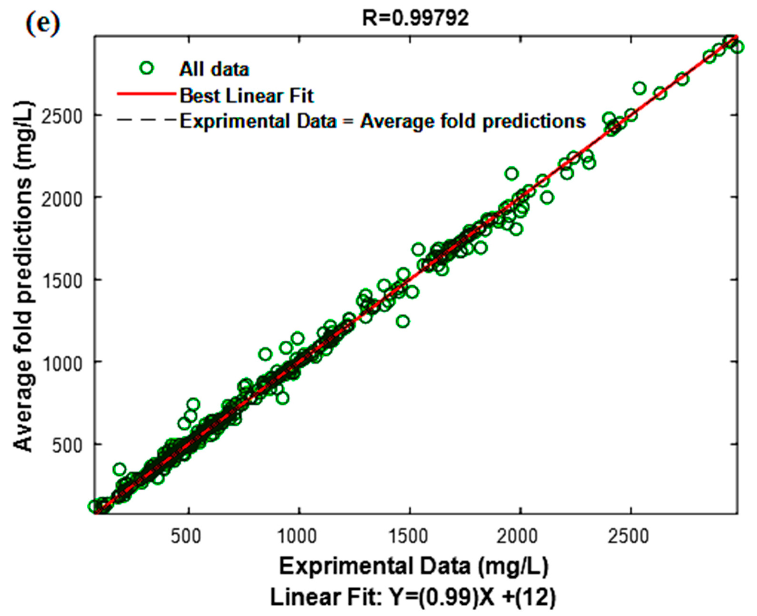
3.3. Model Performance Test

The performance of the model was evaluated by testing it on a pre-existing database of 54 experimental data points that were not used in the model-building process. The pre-existing database was tested on the four best models obtained, and subsequently, the average of the predicted values was calculated. These predicted values were then compared with the corresponding experimental values. The results derived from averaging the outputs of the four models are eloquently displayed in Table 3.
The KNN model consistently demonstrates remarkable performance across all folds, as evidenced by high values of R, R2, and R2adj for each phase. In the training data, the R values range from 0.9930 to 0.9968, indicating strong correlations between the predicted and actual dry residue values. The corresponding R2 values are between 0.9861 and 0.9937, indicating that the model explains a substantial portion of the variance in the training data. Additionally, the R2adj values range from 0.9851 to 0.9932, further confirming the model’s ability to capture the underlying relationships in the data while adjusting for the number of predictors.
For the validation data, the R values range from 0.9948 to 0.9948, indicating consistent predictive ability across the folds. The R2 values range from 0.9848 to 0.9897, suggesting that the model explains a significant proportion of the variance in the validation data. Similarly, the R2adj values range from 0.9809 to 0.9871, indicating a robust performance even after adjusting for the number of predictors.
Furthermore, the values of RMSE and EPM provide insights into the accuracy and precision of the model’s predictions. The RMSE values range from 63.0681 to 110.9024 for the validation data, suggesting that, on average, the predictions deviate from the actual values by a relatively small margin. Similarly, the EPM values range from 3.0832 to 5.1410, indicating the model’s ability to estimate the dry residue values with a high level of accuracy.
It is important to note that the RMSE and EPM values are all relatively low when compared to the optimal experimental value of dry residue, which is 3000 mg/L. This further underscores the effectiveness of the KNN model in accurately predicting the dry residue values. The average results of the outputs from the four models are visually depicted in Figure 3.
Overall, the detailed analysis of the performance metrics for each phase and fold highlights the robustness and accuracy of the KNN model. These results provide strong evidence for the model’s potential to be a valuable tool for analyzing and predicting dry residue values in similar datasets.

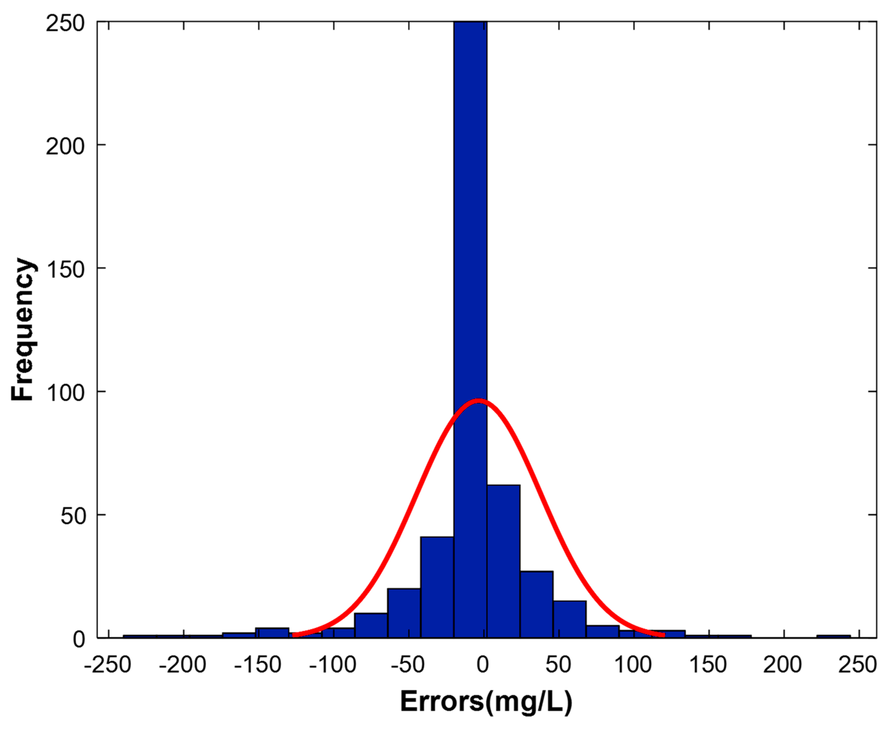
3.4. Analysis of Model Residuals

The residual analysis approach used in this study not only is a widely accepted method for evaluating the performance of regression models but also offers valuable insights that enhance the understanding of the model’s predictive capabilities. By visually comparing the experimental and predicted values, researchers can go beyond numerical metrics and gain a more intuitive understanding of the accuracy and precision of the model’s predictions [8,11]. This visual assessment allows for the identification of any systematic patterns or discrepancies between the observed and predicted values, providing a holistic view of the model’s performance. Moreover, the examination of model residuals through a histogram analysis adds another layer of depth to the evaluation. By grouping the errors into intervals and plotting their frequencies, researchers can explore the distribution of errors and determine if they adhere to certain patterns. In this study, the histogram analysis provides insights into the nature of the errors associated with the KNN model’s predictions. The presence of a normal distribution with a mean of zero suggests that the model’s predictions are unbiased, without any significant tendency to consistently overestimate or underestimate the dry residue values [8,11].
In the specific context of this study, the results of the residual analysis solidify the high performance and reliability of the KNN model in predicting dry residue values. The visual comparison of the experimental and predicted values, as shown in Figure 4, reveals a close match between the two, indicating a strong agreement and demonstrating the model’s ability to capture the underlying patterns and relationships in the data [8,11]. The consistent model performance on the modeling data and on the additional testing data shown in Figure 4 provides crucial insights into the model’s generalization capacity and its consistent performance across different datasets.
Furthermore, Figure 5, displaying the histogram of model errors, reinforces the robustness of the KNN model. The approximate normal distribution of errors around zero implies that the model’s predictions are not skewed towards any specific direction, indicating its stability and reliability across different scenarios. This finding enhances the confidence in the KNN model’s practical applicability, as it suggests that the model can be trusted to provide accurate predictions in real-world settings [8,11,32].
Overall, the comprehensive utilization of residual analysis in this study provides valuable evidence supporting the effectiveness, efficiency, and robustness of the KNN model in predicting dry residue values. The visual comparisons, along with the histogram analysis, enhance the understanding of the model’s performance, ensuring its accuracy, reliability, and practical relevance. These findings have significant implications for both the scientific community and practical applications, contributing to the advancement and utilization of the KNN model in various domains.
Moreover, it is important to note that the residual analysis approach is widely used to evaluate the performance of models in chemistry and other scientific fields. This approach enables the examination of the correlation between predicted and experimental values, and the identification of the sources of errors in the model. By employing this approach, we were able to evaluate the performance of the KNN model in predicting dry residue values accurately. The results of our study suggest that the KNN model is highly effective in predicting dry residue values and can be potentially applied in practical settings. The choice of the “Jaccard” distance metric and “squared inverse” distance weight have also been demonstrated to be optimal for this specific case, and this finding could inform the development of future models in related fields. Overall, the combination of the residual approach and the visualization techniques used in this study provides a comprehensive evaluation of the KNN model’s performance and demonstrates its potential to be used as a reliable tool for predicting dry residue values.

4. Conclusions

In conclusion, this research highlights the importance of modeling water quality and treatment based on the dry residue parameter. The study collected and analyzed water samples from the Médéa region of Algeria, utilizing the K-nearest neighbor (KNN) algorithm combined with the improved grey wolf optimizer (I-GWO) algorithm to predict dry residue content. Rigorous evaluation using cross-validation optimized the models and minimized overfitting risks. The results revealed that the model incorporating the Jaccard distance and the squared inverse weighting function outperformed other models in terms of coefficients and statistical errors across the four folds. Averaging predictions from multiple folds yielded an overall prediction with excellent performance, exhibiting high values for R, R2, R2adj, RMSE, and EPM (0.9979, 0.9958, 0.9956, 41.2639, and 3.1061, respectively). Further testing on an independent dataset consistently confirmed the model’s efficiency and accuracy, demonstrating low error values and a strong correlation coefficient. The model’s effectiveness can be attributed to its ability to capture the non-linear relationship between dry residue content and physico-chemical characteristics of water. Additionally, the successful representation of the data played a crucial role in achieving outstanding performance. Interpolation testing further reinforced the model’s efficiency and correlation coefficient. In summary, this study underscores the importance of incorporating the dry residue parameter in water quality modeling and treatment. The proposed KNN_I-GWO model, which integrates the KNN and I-GWO algorithms and undergoes comprehensive statistical analyses, demonstrated exceptional performance in terms of coefficients and statistical errors. Its accurate representation of the non-linear relationship between dry residue content and physico-chemical characteristics of water holds significant potential for accurately predicting and managing water quality and treatment processes. This research provides valuable insights and contributes to the advancement of water resource management.

Author Contributions

Conceptualization, H.T., S.T., A.H.H.-B., A.B. (Abla Bousselma), A.N.E.H.S., A.-E.B., Z.T., M.K., A.A., J.Z., A.A.A., D.C., A.B. (Abdallah Bouguettoucha) and L.M.; Methodology, H.T., S.T., A.H.H.-B., A.B. (Abla Bousselma), A.N.E.H.S., A.-E.B., Z.T., M.K., A.A., J.Z., A.A.A., D.C. and A.B. (Abdallah Bouguettoucha); Software, H.T., S.T., A.B. (Abla Bousselma), M.K., A.A., J.Z. and A.A.A.; Validation, H.T., S.T., A.H.H.-B., A.B. (Abla Bousselma), A.N.E.H.S., A.-E.B., Z.T., M.K., A.A., J.Z., A.A.A., D.C. and A.B. (Abdallah Bouguettoucha); Formal analysis, H.T., S.T., A.B. (Abla Bousselma), A.N.E.H.S., A.-E.B., Z.T., M.K., A.A., J.Z., A.A.A., D.C. and A.B. (Abdallah Bouguettoucha); Investigation, H.T., S.T., A.H.H.-B., A.N.E.H.S., A.-E.B., Z.T., M.K., A.A., J.Z., D.C., A.B. (Abdallah Bouguettoucha) and L.M.; Resources, H.T., M.K., A.A., J.Z. and A.B. (Abdallah Bouguettoucha); Data curation, H.T., S.T., Z.T., A.A. and J.Z.; Writing—original draft, H.T., S.T., A.N.E.H.S. and M.K.; Writing—review & editing, A.-E.B., Z.T., A.A., J.Z., A.A.A., D.C., A.B. (Abdallah Bouguettoucha) and L.M.; Visualization, H.T., S.T., A.H.H.-B., A.N.E.H.S., A.-E.B., Z.T., M.K., A.A., J.Z., A.A.A., D.C., A.B. (Abdallah Bouguettoucha) and L.M.; Supervision, A.A. and J.Z.; Project administration, H.T., A.A. and J.Z. All authors have read and agreed to the published version of the manuscript.

Funding

This research received no external funding.

Conflicts of Interest

The authors declare no conflict of interest.

References

  1. Kılıç, Z. The Importance of Water and Conscious Use of Water. Int. J. Hydrol. 2020, 4, 239–241. [Google Scholar] [CrossRef]
  2. Deng, W.; Wang, G.; Zhang, X. A Novel Hybrid Water Quality Time Series Prediction Method Based on Cloud Model and Fuzzy Forecasting. Chemom. Intell. Lab. Syst. 2015, 149, 39–49. [Google Scholar] [CrossRef]
  3. Hamid, A.; Bhat, S.U.; Jehangir, A. Local Determinants Influencing Stream Water Quality. Appl. Water Sci. 2020, 10, 24. [Google Scholar] [CrossRef] [Green Version]
  4. Ding, Y.R.; Cai, Y.J.; Sun, P.D.; Chen, B. The Use of Combined Neural Networks and Genetic Algorithms for Prediction of River Water Quality. J. Appl. Res. Technol. 2014, 12, 493–499. [Google Scholar] [CrossRef]
  5. Ho, J.Y.; Afan, H.A.; El-Shafie, A.H.; Koting, S.B.; Mohd, N.S.; Jaafar, W.Z.B.; Lai Sai, H.; Malek, M.A.; Ahmed, A.N.; Mohtar, W.H.M.W.; et al. Towards a Time and Cost Effective Approach to Water Quality Index Class Prediction. J. Hydrol. 2019, 575, 148–165. [Google Scholar] [CrossRef]
  6. Tahraoui, H.; Amrane, A.; Belhadj, A.-E.; Zhang, J. Modeling the Organic Matter of Water Using the Decision Tree Coupled with Bootstrap Aggregated and Least-Squares Boosting. Environ. Technol. Innov. 2022, 27, 102419. [Google Scholar] [CrossRef]
  7. Tahraoui, H.; Belhadj, A.-E.; Triki, Z.; Boudella, N.R.; Seder, S.; Amrane, A.; Zhang, J.; Moula, N.; Tifoura, A.; Ferhat, R.; et al. Mixed Coagulant-Flocculant Optimization for Pharmaceutical Effluent Pretreatment Using Response Surface Methodology and Gaussian Process Regression. Process Saf. Environ. Prot. 2022, 169, 909–927. [Google Scholar] [CrossRef]
  8. Tahraoui, H.; Belhadj, A.-E.; Amrane, A.; Houssein, E.H. Predicting the Concentration of Sulfate Using Machine Learning Methods. Earth Sci. Inform. 2022, 15, 1023–1044. [Google Scholar] [CrossRef]
  9. Collivignarelli, M.C.; Abbà, A.; Benigna, I.; Sorlini, S.; Torretta, V. Overview of the Main Disinfection Processes for Wastewater and Drinking Water Treatment Plants. Sustainability 2017, 10, 86. [Google Scholar] [CrossRef] [Green Version]
  10. Tahraoui, H.; Belhadj, A.-E.; Hamitouche, A.-E. Prediction of the Bicarbonate Amount in Drinking Water in the Region of Médéa Using Artificial Neural Network Modelling. Kem. U Ind. Časopis Kemičara Kem. Inženjera Hrvat. 2020, 69, 595–602. [Google Scholar] [CrossRef]
  11. Tahraoui, H.; Belhadj, A.-E.; Hamitouche, A.-E.; Bouhedda, M.; Amrane, A. Predicting the Concentration of Sulfate (So4 2–) in Drinking Water Using Artificial Neural Networks: A Case Study: Médéa-Algeria. Desalination Water Treat. 2021, 217, 181–194. [Google Scholar] [CrossRef]
  12. Rajaee, T.; Khani, S.; Ravansalar, M. Artificial Intelligence-Based Single and Hybrid Models for Prediction of Water Quality in Rivers: A Review. Chemom. Intell. Lab. Syst. 2020, 200, 103978. [Google Scholar] [CrossRef]
  13. Hastie, T.; Tibshirani, R.; Friedman, J.H.; Friedman, J.H. The Elements of Statistical Learning: Data Mining, Inference, and Prediction; Springer: Berlin/Heidelberg, Germany, 2009; Volume 2. [Google Scholar]
  14. Amendolia, S.R.; Cossu, G.; Ganadu, M.L.; Golosio, B.; Masala, G.L.; Mura, G.M. A Comparative Study of K-Nearest Neighbour, Support Vector Machine and Multi-Layer Perceptron for Thalassemia Screening. Chemom. Intell. Lab. Syst. 2003, 69, 13–20. [Google Scholar] [CrossRef]
  15. Altman, N.S. An Introduction to Kernel and Nearest-Neighbor Nonparametric Regression. Am. Stat. 1992, 46, 175–185. [Google Scholar]
  16. Kotsiantis, S.B.; Zaharakis, I.; Pintelas, P. Supervised Machine Learning: A Review of Classification Techniques. Emerg. Artif. Intell. Appl. Comput. Eng. 2007, 160, 3–24. [Google Scholar]
  17. Alpaydin, E. Introduction to Machine Learning; MIT Press: Cambridge, MA, USA, 2020; ISBN 0-262-04379-3. [Google Scholar]
  18. Zamouche, M.; Chermat, M.; Kermiche, Z.; Tahraoui, H.; Kebir, M.; Bollinger, J.-C.; Amrane, A.; Mouni, L. Predictive Model Based on K-Nearest Neighbor Coupled with the Gray Wolf Optimizer Algorithm (KNN_GWO) for Estimating the Amount of Phenol Adsorption on Powdered Activated Carbon. Water 2023, 15, 493. [Google Scholar] [CrossRef]
  19. Adithiyaa, T.; Chandramohan, D.; Sathish, T. Optimal Prediction of Process Parameters by GWO-KNN in Stirring-Squeeze Casting of AA2219 Reinforced Metal Matrix Composites. Mater. Today Proc. 2020, 21, 1000–1007. [Google Scholar] [CrossRef]
  20. Huang, H.; Wang, Q.; He, X.; Wu, Y.; Xu, C. Association between Polyfluoroalkyl Chemical Concentrations and Leucocyte Telomere Length in US Adults. Sci. Total Environ. 2019, 653, 547–553. [Google Scholar] [CrossRef]
  21. Uddin, M.G.; Nash, S.; Olbert, A.I. A Review of Water Quality Index Models and Their Use for Assessing Surface Water Quality. Ecol. Indic. 2021, 122, 107218. [Google Scholar] [CrossRef]
  22. Rodier, J.; Legube, B.; Merlet, N.; Brunet, R. L’analyse de L’eau-9e éd.: Eaux Naturelles, Eaux Résiduaires, Eau de Mer; Dunod: Malakoff Cedex, France, 2009; ISBN 978-2-10-054179-9. [Google Scholar]
  23. Sinha, P.; Sinha, P. Comparative Study of Chronic Kidney Disease Prediction Using KNN and SVM. Int. J. Eng. Res. 2015, 4, 608–612. [Google Scholar] [CrossRef]
  24. Ahmed, R.; Rangaiah, G.P.; Mahadzir, S.; Mirjalili, S.; Hassan, M.H.; Kamel, S. Memory, Evolutionary Operator, and Local Search Based Improved Grey Wolf Optimizer with Linear Population Size Reduction Technique. Knowl.-Based Syst. 2023, 110297. [Google Scholar] [CrossRef]
  25. Seyyedabbasi, A.; Kiani, F. I-GWO and Ex-GWO: Improved Algorithms of the Grey Wolf Optimizer to Solve Global Optimization Problems. Eng. Comput. 2021, 37, 509–532. [Google Scholar] [CrossRef]
  26. Yahoum, M.M.; Toumi, S.; Hentabli, S.; Tahraoui, H.; Lefnaoui, S.; Hadjsadok, A.; Amrane, A.; Kebir, M.; Moula, N.; Assadi, A.A. Experimental Analysis and Neural Network Modeling of the Rheological Behavior of Xanthan Gum and Its Derivatives. Materials 2023, 16, 2565. [Google Scholar] [CrossRef] [PubMed]
  27. Belsley, D.A.; Kuh, E.; Welsch, R.E. Regression Diagnostics: Identifying Influential Data and Sources of Collinearity; Wiley: Hoboken, NJ, USA, 1980; ISBN 978-0-471-05856-4. [Google Scholar]
  28. Hong, S.H.; Lee, M.W.; Lee, D.S.; Park, J.M. Monitoring of Sequencing Batch Reactor for Nitrogen and Phosphorus Removal Using Neural Networks. Biochem. Eng. J. 2007, 35, 365–370. [Google Scholar] [CrossRef]
  29. Bousselma, A.; Abdessemed, D.; Tahraoui, H.; Amrane, A. Artificial Intelligence and Mathematical Modelling of the Drying Kinetics of Pre-Treated Whole Apricots. Kem. U Ind. 2021, 70, 651–667. [Google Scholar] [CrossRef]
  30. Bouchelkia, N.; Tahraoui, H.; Amrane, A.; Belkacemi, H.; Bollinger, J.-C.; Bouzaza, A.; Zoukel, A.; Zhang, J.; Mouni, L. Jujube Stones Based Highly Efficient Activated Carbon for Methylene Blue Adsorption: Kinetics and Isotherms Modeling, Thermodynamics and Mechanism Study, Optimization via Response Surface Methodology and Machine Learning Approaches. Process. Saf. Environ. Prot. 2022, 170, 513–535. [Google Scholar] [CrossRef]
  31. Zamouche, M.; Tahraoui, H.; Laggoun, Z.; Mechati, S.; Chemchmi, R.; Kanjal, M.I.; Amrane, A.; Hadadi, A.; Mouni, L. Optimization and Prediction of Stability of Emulsified Liquid Membrane (ELM): Artificial Neural Network. Processes 2023, 11, 364. [Google Scholar] [CrossRef]
  32. Tahraoui, H.; Belhadj, A.-E.; Moula, N.; Bouranene, S.; Amrane, A. Optimisation and Prediction of the Coagulant Dose for the Elimination of Organic Micropollutants Based on Turbidity. Kem. U Ind. 2021, 70, 675–691. [Google Scholar] [CrossRef]
  33. Manssouri, I.; Manssouri, M.; El Kihel, B. Fault Detection by K-Nn Algorithm and Mlp Neural Networks in a Distillation Column: Comparative Study. J. Inf. Intell. Knowl. 2011, 3, 201. [Google Scholar]
  34. Manssouri, I.; El Hmaidi, A.; Manssouri, T.E.; El Moumni, B. Prediction Levels of Heavy Metals (Zn, Cu and Mn) in Current Holocene Deposits of the Eastern Part of the Mediterranean Moroccan Margin (Alboran Sea). IOSR J. Comput. Eng. 2014, 16, 117–123. [Google Scholar] [CrossRef]
  35. Dolling, O.R.; Varas, E.A. Artificial Neural Networks for Streamflow Prediction. J. Hydraul. Res. 2002, 40, 547–554. [Google Scholar] [CrossRef]
  36. Post, G.B.; Atherholt, T.B.; Cohn, P.D. Water quality and treatment: A handbook on drinking water. In Health and Aesthetic Aspects of Drinking Water, 6th ed.; McGraw-Hill: New York, NY, USA, 2011; pp. 2.1–2.100. [Google Scholar]
  37. Boyd, C.E. Water Quality: An Introduction; Springer Nature: Berlin/Heidelberg, Germany, 2019; ISBN 3-030-23335-9. [Google Scholar]
  38. Bartram, J.; Ballance, R. Water Quality Monitoring: A Practical Guide to the Design and Implementation of Freshwater Quality Studies and Monitoring Programmes; CRC Press: Boca Raton, FL, USA, 1996; ISBN 0-419-22320-7. [Google Scholar]
  39. WHO. Guidelines for Drinking-Water Quality; World Health Organization: Geneva, Switzerland, 2004; Volume 1, ISBN 92-4-154638-7. [Google Scholar]
  40. Staff, A. Water Quality: Principles and Practices of Water Supply Operations; American Water Works Assoc.: Denver, CO, USA, 2003. [Google Scholar]
  41. Csuros, M.; Csuros, C. Environmental Sampling and Analysis for Metals; CRC Press: Boca Raton, FL, USA, 2016; ISBN 1-4200-3234-8. [Google Scholar]
  42. Rice, E.W.; Bridgewater, L.; Association, A.P.H. Standard Methods for the Examination of Water and Wastewater; American Public Health Association: Washington, DC, USA, 2012; Volume 10. [Google Scholar]
  43. Nollet, L.M.; De Gelder, L.S. Handbook of Water Analysis; CRC Press: Boca Raton, FL, USA, 2000; ISBN 0-8493-8486-9. [Google Scholar]
  44. Graindorge, J.; Landot, É. La Qualité de L’eau Potable: Techniques et Responsabilités; Territorial éditions; Territorial: Voiron, France, 2018; ISBN 2-8186-1418-X. [Google Scholar]
  45. Debieche, T.H. Evolution de La Qualité Des Eaux (Salinité, Azote et Métaux Lourds) Sous L’effet de la Pollution Saline, Agricole et Industrielle: Application à la Basse Plaine de la Seybouse Nord-Est Algérien; University of Franche-Comté: Besançon, France, 2002. [Google Scholar]
  46. Bishop, C.M.; Nasrabadi, N.M. Pattern Recognition and Machine Learning; Springer: Berlin/Heidelberg, Germany, 2006; Volume 4. [Google Scholar]
  47. Murphy, K.P. Machine Learning: A Probabilistic Perspective; MIT Press: Cambridge, MA, USA, 2012; ISBN 0-262-30432-5. [Google Scholar]
Figure 1. Organization chart for the development and optimization of the KNN_I-GWO model.
Water 15 02631 g001
Figure 2. Comparison between experimental and predicted values: (a) 1st fold, (b) 2nd fold, (c) 3rd fold, (d) 4th fold, and (e) the average of the models in the 4 folds.
Water 15 02631 g002aWater 15 02631 g002bWater 15 02631 g002cWater 15 02631 g002dWater 15 02631 g002e
Figure 3. Relationship between experimental and predicted values to assess performance.
Water 15 02631 g003
Figure 4. Experimental and predicted values for the modeling samples (samples 1 to 400) and testing samples (samples 401 to 454).
Water 15 02631 g004
Figure 5. Histogram of model errors.
Water 15 02631 g005
Table 1. The model inputs and output with statistical analysis.
VariablesSymbolUnitMinMeanMaxSTD
Inputs
ConductivityX1µS/cm2231263.983570754.59
TurbidityX2NTU0.107.87102458.57
Potential hydrogenX32.109.6279737.07
HardnessX4mg/L8.1353.4216024.27
CalciumX5mg/L16.03121.87360.7247.40
MagnesiumX6mg/L055.20218.7036.91
Total alkalimetric titreX7°F6.50117.71663133.39
BicarbonateX8mg/L6.74200.11495.20117.01
ChloridesX9mg/L10.50150.76609.39125.91
Nitrogen dioxideX10mg/L00.010.500.07
AmmoniumX11mg/L00.021.050.14
NitratesX12mg/L08.13195.0915.89
PhosphateX13mg/L01.2828819.09
SulfateX14mg/L10.55342.251457287.37
SodiumX15mg/L0122.05460121.67
PotassiumX16mg/L0.0056.9280537.92
ManganeseX17mg/L00.0070.210.02
IronX18mg/L00.0130.530.03
AluminumX19mg/L00.0050.900.04
Organic matterX20mg/L03.2629.203.86
Output
Dry residueYmg/L29916.012980635.64
Table 2. Performances of the best model.
Number of
Neighbors
R/R2/R2adjRMSE/EPM
TrainVALALLTrainVALALL
1st fold
30.99580.9951 0.995656.000070.200059.9000
0.99160.9902 0.99112.70003.20002.8000
0.99100.98770.9907
2nd fold
50.99480.99240.994165.800079.300069.4000
0.98960.9848 0.98823.20004.30003.5000
0.98880.98090.9876
3rd fold
60.99680.98800.994048.5000110.900069.5000
0.99370.97610.98812.20005.10002.9000
0.99320.97000.9874
4th fold
70.9930 0.99480.993575.700063.000072.7000
0.98610.98970.98693.00003.80003.2000
0.98510.98710.9863
The average of the folds
///0.9979//41.2000
0.99583.1000
0.9956
Table 3. Model test performance.
R R2R2adjRMSEEPM
0.99010.98040.968587.70009.6000
Disclaimer/Publisher’s Note: The statements, opinions and data contained in all publications are solely those of the individual author(s) and contributor(s) and not of MDPI and/or the editor(s). MDPI and/or the editor(s) disclaim responsibility for any injury to people or property resulting from any ideas, methods, instructions or products referred to in the content.

