
Shape Factor for Analysis of a Slug Test

Department of Hydrology and Hydraulic Engineering, Vrije Universiteit Brussel, Pleinlaan 2, 1050 Brussels, Belgium
Water 2023, 15(14), 2551; https://doi.org/10.3390/w15142551
Submission received: 18 May 2023
/
Revised: 3 July 2023
/
Accepted: 9 July 2023
/
Published: 12 July 2023
(This article belongs to the Special Issue Groundwater Exploration and Hydrogeophysical Research)
Abstract
:Hydraulic conductivity is an essential parameter for groundwater investigation and management. A simple technique for determining the hydraulic conductivity of aquifers is the slug test, which consists of measuring the water level in a well after the sudden removal or injection of a small amount of water. The interpretation of a slug test is based on a geometry-dependent shape factor, for which various empirical relationships and approximate solutions have been proposed in the literature. In this study, shape factors are derived numerically for slug tests performed in monitoring wells with screens unaffected by aquifer boundaries. Also presented is a new approximate analytical solution for predicting shape factors for well screens with a large aspect ratio. A comparison with earlier methods reported in the literature shows that our results match or exceed them in terms of accuracy. The approximate analytical solution is promising because it is accurate and very easy to apply in practice.
1. Introduction
Hydraulic conductivity describes the ease with which water can move through porous materials, which is an essential factor for groundwater exploration and management. The hydraulic conductivity of ground layers can be obtained by laboratory testing on soil samples or by field testing in groundwater wells or boreholes. Most accurate are pumping tests carried out in wells, which, however, require a lot of effort and resources. On the other hand, slug tests performed in monitoring wells or double-packer boreholes allow the hydraulic conductivity of soil layers to be obtained more quickly and easily, because only one well is required, no pumping is needed, and the test can usually be completed within a short period of time. However, aquifer parameters obtained from slug tests are less representative than from pumping tests, because only a small volume of the aquifer is tested, i.e., the soil surrounding the well screen, and in addition complications such as well skin, soil anisotropy, water and soil compressibility, or inertial effects may occur. Nevertheless, despite these drawbacks, slug tests can still yield valuable insights into the hydraulic properties of aquifers, when properly used and interpreted and in combination with other site characterization techniques.
A slug test consists of estimating the hydraulic conductivity from observations of the recovery of the water level in a well after a sudden removal or injection of a small amount of water. There is no exact mathematical solution to this problem, but it is generally accepted that, ignoring the elastic storage in the aquifer, the head difference in the well decays exponentially with time, as proposed by Hvorslev [1] and Bouwer and Rice [2] as follows:
where [L] is the head difference in the well at time [T] since the start of the test, is the initial change in head induced in the well at time zero, [L] is the length of the well screen, [LT−1] is the hydraulic conductivity of the soil, [L] is the inner radius of the well tubing where the head difference is observed, [L] is an effective radius, and [L] is the outer radius of the well screen (including a gravel pack if present). The hydraulic conductivity of the soil can thus be obtained by analyzing the slope of the logarithm of the observed head values against time [1,2] as
where ln is the natural logarithm. Since the method is only approximate, observations may deviate from the assumed behavior, so in practice only the slope of the longest rectilinear part of versus measurements is used for the analysis [3].
The effective radius in Equations (1) and (2) is essentially a model parameter, representing the radial distance from the center of the well at which the induced hydraulic head change in the soil around the well becomes negligible. It is determined by the configuration of the groundwater flow around the well screen, which depends on the physical dimensions of the well screen and the type and boundary conditions of the aquifer. When sufficiently far from the boundaries of the aquifer, the effective radius depends only on the length and outer diameter of the well screen. In practice, it is more convenient to report values or expressions for , which is commonly denoted as the shape factor. Exact derivations of the effective radius or shape factor have not yet been found and one must rely on various approximations reported in the literature. Approximate values and expressions have been determined by electric analog models, e.g., [2,4]; numerical groundwater flow models, e.g., [5,6,7]; or approximate analytical solutions, e.g., [1,8,9,10,11,12,13,14,15]. All approaches have their merits, but none are conclusive in the sense of being more accurate or superior to others.
The most commonly used Is the Hvorslev method [1], based on a simple analytical approximation assuming uniform flow at the well screen, e.g., [16], leading to the following expression for the shape factor:
where sinh−1 is the inverse hyperbolic sine function. For a well screen with a large aspect ratio (), this can be further simplified as
showing that the effective radius is equal to the length of the well screen if the length is much larger than the outer radius of the well screen, which is usually the case in practice. Also very popular is the approach of Bouwer and Rice [2], who presented, by electric analog modeling, empirical expressions with coefficients in graphical form for the shape factor of slug tests conducted in a phreatic aquifer as a function of the dimensions of the well screen and the distance to the water table and impervious base of the aquifer. Recently, Zlotnik et al. [13] presented an approximate analytical solution to the same problem in the form of an infinite series, assuming that the groundwater flow along the well screen is uniform. Table 1 summarizes the key assumptions and techniques of these approaches and of the methods proposed in this study. More discussions and reviews on the assumptions, approximations, and practicality of these methods can be found in the literature, e.g., [5,17,18,19,20,21,22].
The purpose of this work is to derive accurate values for the shape factor of slug tests performed in groundwater monitoring wells with screen dimensions that are commonly found in practice, and to assess the accuracy of other existing analysis methods for slug tests (Table 1). Our approach is performed in two ways: (1) a precise numerical solution and (2) an approximate closed-form analytic solution for well screens with a small aspect ratio. Both techniques derive shape factors for slug tests performed in wells unaffected by aquifer boundary conditions, but accounting for non-uniform flux conditions at the well screen. It is shown that the approximate analytic solution is accurate and easy to apply in practice.
2. Materials and Methods
Consider a slug test performed in a well with a screened section as shown schematically in Figure 1. It is assumed that this is a groundwater monitoring well, often also referred to as a piezometer, with small screen dimensions as is usually the case in practice. When a slug of water is injected or removed from the well, water flowing through the screen compensates for the induced head difference. From the mass balance of water in the well, it follows that
where [L] is the half-length of the screen, [-] is the specific flux passing through the screen, and is the average specific flux over the well screen; by specific flux we mean flux divided by hydraulic conductivity, which is equal to minus the hydraulic gradient. From Equation (1) we also have
Combining these equations, it follows that
which shows that the effective radius or shape factor can be derived from the dimensions of the well screen, the ratio of the difference in head in the well, and the average specific flux passing through the well screen.
To find the average specific flux, we need to solve the groundwater flow equation given by
where [L] is the hydraulic potential in the soil, [L] is the radial distance from the center of the well, and [L] is the elevation measured from the center of the screen. Note that there is no storage term in the groundwater flow equation because the aquifer and groundwater are assumed to be incompressible. This means that, although the hydraulic potential and flux vary with time, the groundwater flow is in a (pseudo-)steady state at any point in time. The boundary conditions are
where the well screen is assumed to be located far from the aquifer boundaries, so aquifer boundary conditions can be ignored. Note that a mixed type of boundary value problem is obtained (head condition on the well screen and flux condition on the well tubing). In general, such problems are very difficult, almost impossible to solve exactly.
Using the Fourier cosine transform and back-transformation, the following relation is obtained, e.g., [8,9,12,23,24]:
where and are the modified Bessel functions of the second kind of order zero and one, respectively. If Equation (12) is applied to the screen , it follows that
The problem is thus converted into a Fredholm integral equation of the first kind. In general, such problems are also very difficult to solve exactly and one has to resort to numerical techniques or approximate solutions.
3. Results
3.1. Numerical Solution
The first approach involves a numerical solution to the problem as follows. The upper half part of the well screen is divided into sections of uniform thickness . The specific flux in each section is assumed to be uniform, so Equation (14) becomes
This can be solved iteratively by relaxation:
where is the iteration level and is a relaxation parameter, which has to be specified by trial and error to control the convergence of the iteration procedure. Strong under-relaxation is required () to ensure the stability and convergence of the iterative procedure as Fredholm integral equations of the first kind are ill posed, so small perturbations can strongly affect the convergence.
The approximate solution given by Equation (22) is used as a starting value for the iteration. The effective radius is then obtained from Equation (7) as
3.2. Approximate Analytical Solution
The second approach involves an approximate analytical solution derived as follows. The G-function given by Equation (13) tends to infinity when goes to zero, so Equation (14) can be approximated by the first term of an asymptotic expansion as
This can be further simplified by considering that the radius of the screen is usually much smaller than the length, so in Equation (13) can be approximated as , so
and Equation (19) can be simplified as
This can also be written as
Compared to Equation (7), the left side of Equation (22) can be interpreted as a local shape factor at elevation z along the well screen, and, instead of using the average specific flux, we will derive the overall shape factor by averaging the local shape factors over the well screen so that
which leads to the following expression for the shape factor:
For a well screen with a large aspect ratio (), this can be further simplified as
which shows that the effective radius for large aspect ratios of the screen is smaller than the screen length, contrary to what was suggested by Hvorslev [1]. Equation (25) has been previously reported by Wilkinson and Hammond [8].
3.3. Shape Factor Values
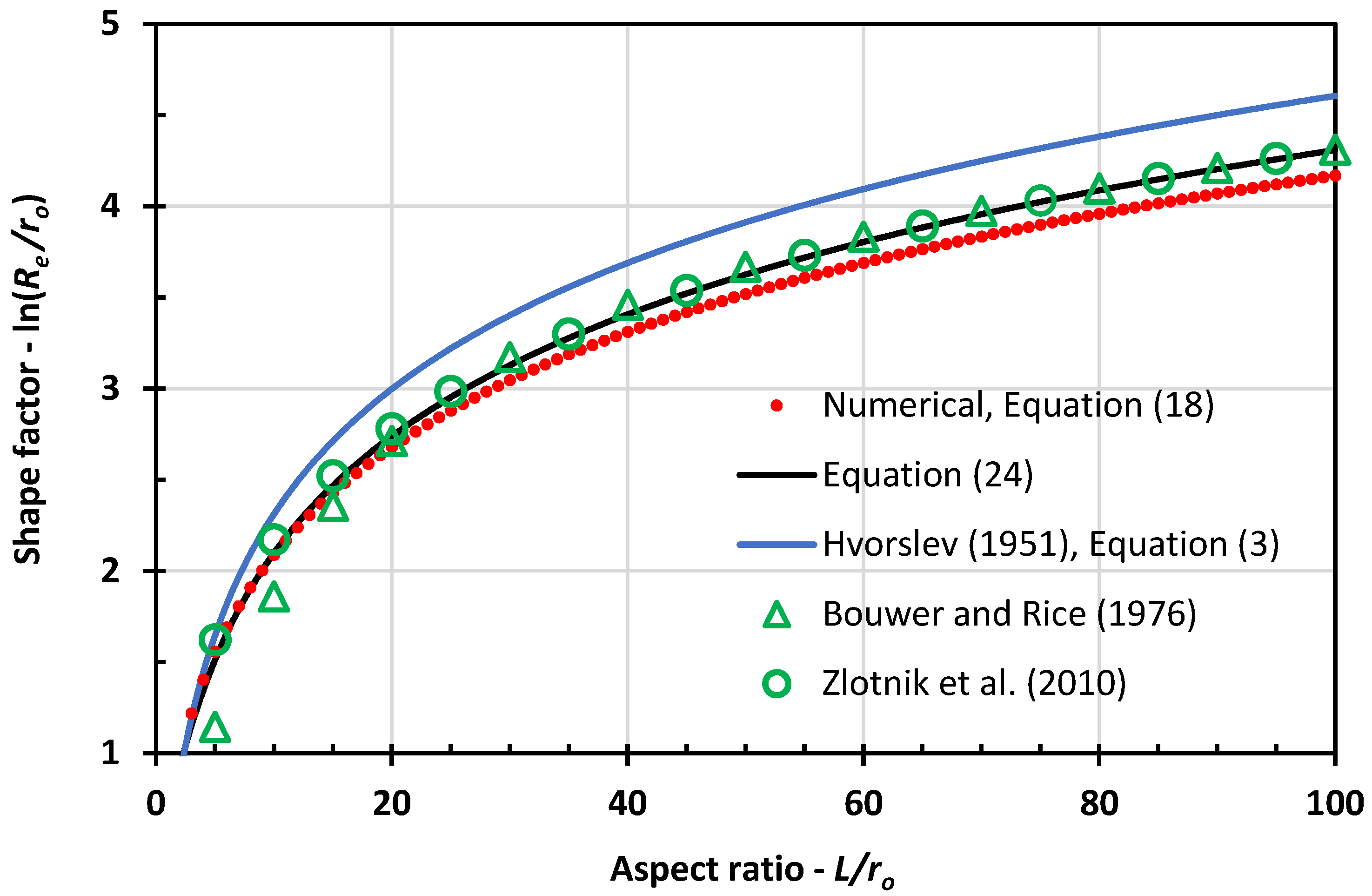
The shape factors were derived with different approaches: (1) numerical approach using Equations (17) and (18), (2) approximate analytical solution given by Equation (24), (3) Hvorslev approach [1] given by Equation (3), (4) Bouwer and Rice empirical approach [2], and (5) the approximate solution of Zlotnik et al. [13]. The results are shown in Figure 2.
For the numerical approach, the specific flux along the well screen is derived with Equation (17) for screen aspect ratios ranging from 1 to 100 by dividing the half length of the screen into 1000 intervals of equal length. The asymptotic analytical solution given by Equation (22) is used as a starting value for the iterative solution procedure. A relation factor is used in the iteration procedure and several hundred iterations are needed until the improvements for all values become smaller than 10−5. These values are used to derive the average specific flux value along the well screen and the resulting shape factor using Equation (18).
The shape factors for the approximate analytical solution were derived with Equation (24). For the Bouwer and Rice empirical approach [2] and the approximate solution of Zlotnik et al. [13], we used computer codes from Zlotnik et al. [13], where the coefficients in graphical form of the Bouwer and Rice approach [2] are calculated with the polynomial curve fittings of Yang and Yeh [25]. To avoid the influence of aquifer boundary conditions, we considered a well screen with a length of 2 m and a varying outer radius, placed in the middle of a 100 m thick phreatic aquifer.
The shape factors plotted in Figure 2 against the aspect ratio of the well screen appear to be very close except for the Hvorslev method [1]. The differences between the methods except Hvorslev’s are less than 4%; the Bouwer and Rice [2] values for aspect ratios less than 15 deviate somewhat more. The values of the Hvorslev approach [1] deviate the most, about 10%, from the other methods. Considering the numerical approach as the most accurate, it can be concluded that the approximate analytical solution given by Equation (24) and the Zlotnik et al. [13] and Bouwer and Rice approaches [2] are accurate and acceptable for real-world slug test analysis. As such, Equation (24) has the merit of being the simplest and therefore more suitable for practical use, but, conversely, is only valid for slug tests performed in wells with screens unaffected by aquifer boundaries.
3.4. Test Case
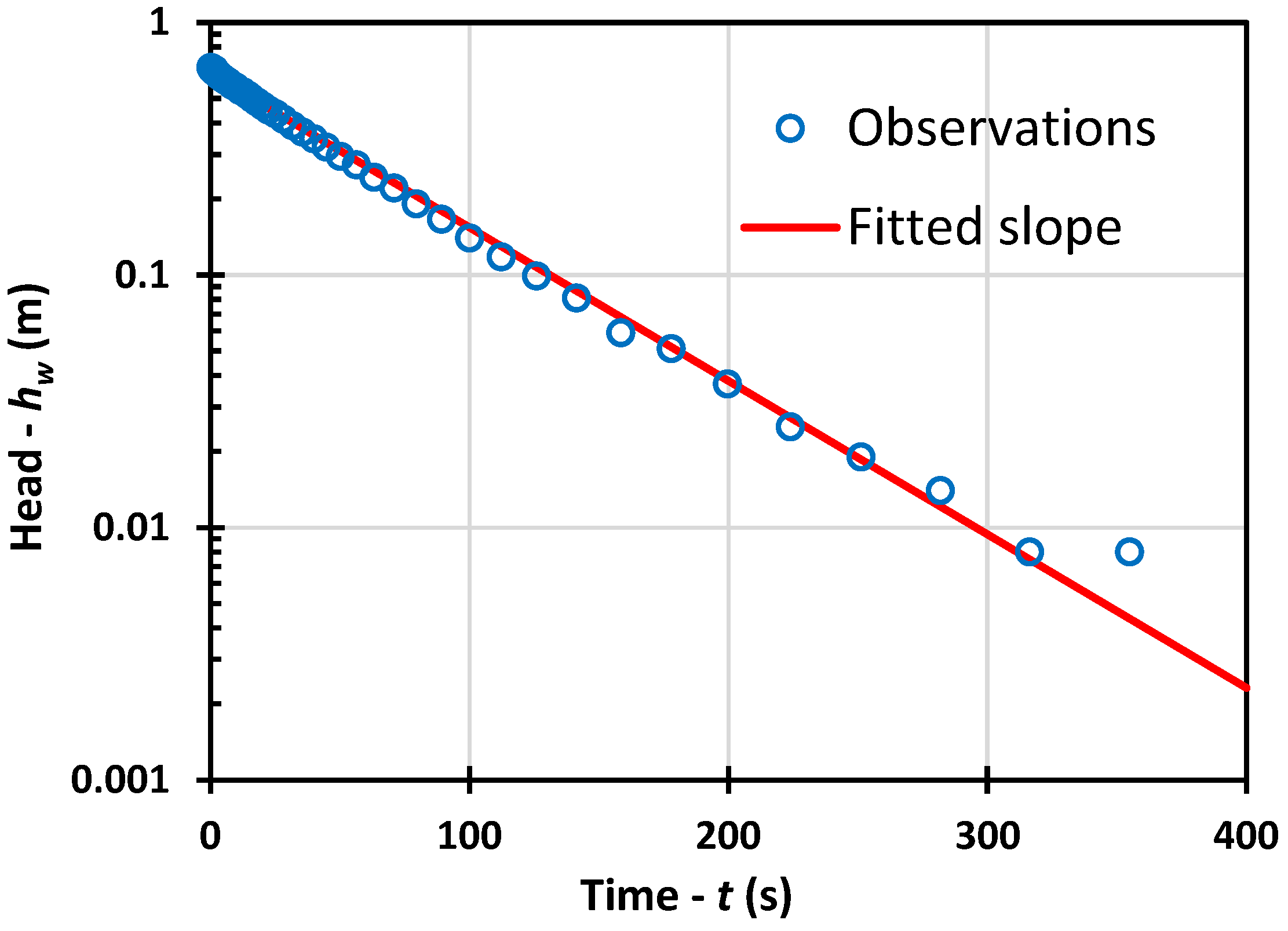
To demonstrate the usefulness of the methodology, it was applied to a practical test case taken from Butler [21]. The test case consisted of a falling head slug test conducted in a monitoring well, Well 4-2 in Pratt County Monitoring Site 36, Kansas, U.S. The aquifer is unconfined and consists mainly of unconsolidated alluvial deposits of sand and gravel with interbedded clay. At the well site, the aquifer is 47.87 m thick. The top of the well filter section is located at a depth of 16.77 m below the static water level. The well has an inner radius ri = 0.064 m, an outer radius ro = 0.125 m, and a length L = 1.52 m. The initial head displacement in the well was h0 = 0.671 m and the difference in head hw was monitored for about 6 min. The observations against time are shown in Figure 3.
The hydraulic conductivity of the aquifer is estimated using Equation (2). The slope of the logarithm of the observed head values versus time, determined by linear regression, is −0.014 s−1, as shown in Figure 3. Values for the shape factor obtained with the different methods are given in Table 2. The resulting shape factors are very similar, plausibly because the well screen is located far from the boundaries of the aquifer. The last column of Table 2 gives the resulting estimates of the hydraulic conductivity of the aquifer. All methods more or less agree, but the values obtained by the methods prosed in this study and the method of Zlotnik et al. [13] are very close to each other, while the value obtained with the Hvorslev method [1] is clearly larger and the value obtained with the method of Bouwer and Rice [2] is clearly lower. Hence, this practical example confirms the conclusions from the previous section and clearly demonstrates the applicability and accuracy of the methodology proposed in this study.
4. Discussion
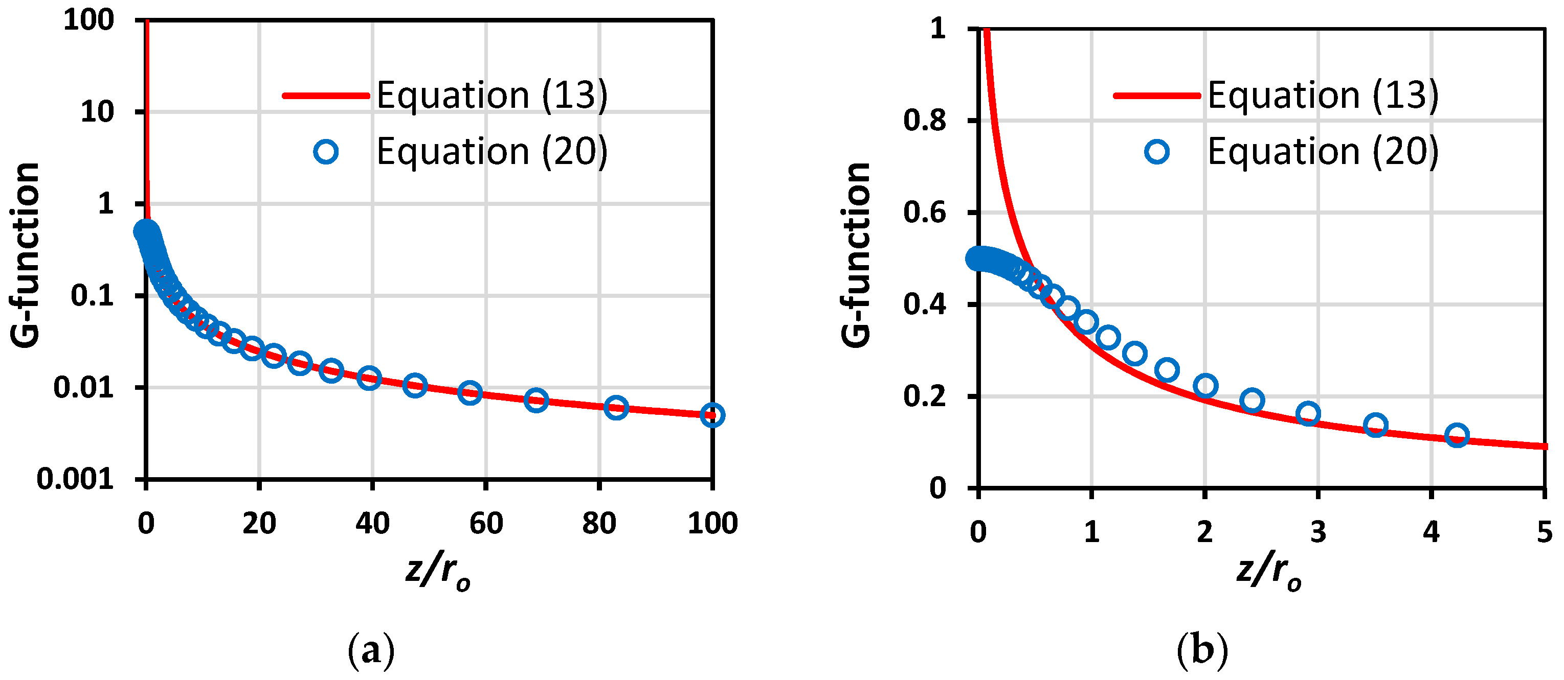
The approximate analytical solution given by Equation (24) is derived based on some assumptions that enable a simple expression to be obtained for the shape factor that can be easily applied in practice. The first assumption is that the G-function has a strong peak at the origin, which allows Equation (14) to be approximated by the leading term of an asymptotic expansion. Figure 4 shows a graph of the G-function against as given by Equation (13) and the approximation for large aspect ratios given by Equation (20). Figure 4a shows a general view using a semilogarithmic plot, while Figure 4b shows details near the origin on a linear plot. The two equations generally overlap, except near the origin where the exact solution, Equation (13), tends to infinity, while the approximate solution, Equation (20), is finite at the origin with a value of 1/2. Either way, both solutions peak and reach their maximum at the origin, which justifies the approximation of the integral in Equation (14) by asymptotic expansion.
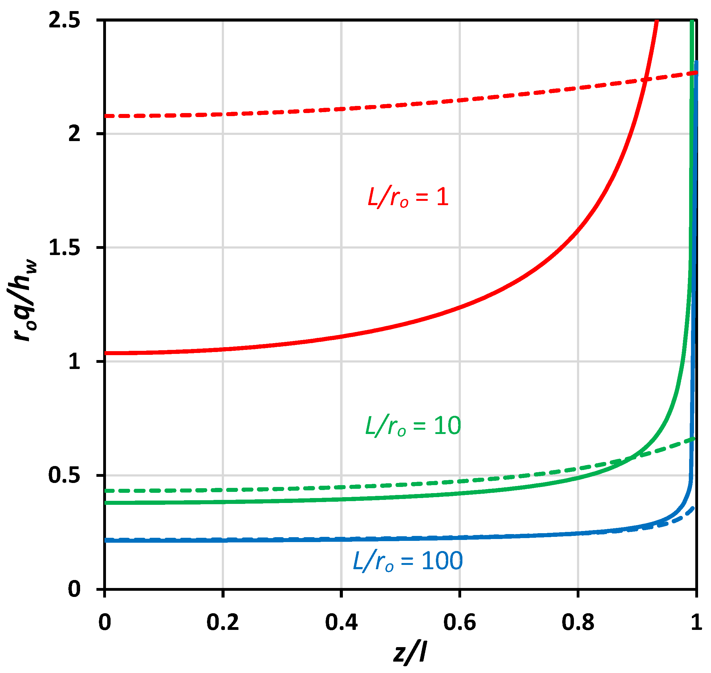
The accuracy of the approximate analytical solution also depends on deriving the shape factor by averaging the local shape factors instead of using the average specific flux. The error introduced by this assumption depends on the degree of uniformity of the specific flux along the well screen and will be small if the flux distribution is more uniform. Figure 5 shows a plot of against derived with the numerical solution, Equation (17) (solid lines), and with the approximate analytical solution, Equation (22) (dotted lines), for the screen aspect ratios equal to 1, 10, and 100, respectively. Similar derivations of flux distributions along the screen have been presented in other studies [5,10,15,23,26,27,28,29]. The flux derived with the asymptotic approximation appears to be fairly uniform along the screen, while the flux derived with the numerical solution is less uniform, especially for small aspect ratios, and tends to infinity at the edges of the screen (). It seems that for the screen ratio going to infinity, the flux becomes completely uniform with Dirac peaks at the edges. The physical explanation for this is that the flux vector must be perpendicular to the screen because the screen forms an iso-potential surface but must be parallel to the impermeable casing of the well outside the screen, resulting in a singularity at the edges of the screen with an infinite flux vector. This singularity is probably one of the reasons that an exact analytical solution is difficult to obtain and also represents a major obstacle to the accurate modelling of groundwater flow using numerical techniques, which has often been overlooked in the literature, e.g., [4,5,15,20,26].
Thus, the asymptotic approximation for the specific flux is fairly uniform, but differs from the more accurate numerical solution, especially for small aspect ratios and near the edges of the screen, where it does not tend to infinity but reaches a finite value. However, to compensate for this, the approximate flux values are slightly larger than those obtained with the numerical solution, except near the edges, so the total flow through the screen becomes more or less equal to what is obtained with the numerical solution, resulting in a similar shape factor.
The final assumption in the derivation of the approximate analytical solution is that the aspect ratio of the well screen is large, which in practice is usually the case for groundwater monitoring wells because the length of the screen is typically in the order of meters and the radius in the order of centimeters, which is one to two orders of magnitude smaller. Hence, the assumptions leading to the approximate analytical solution are acceptable in practice, and the results shown in Figure 2 prove that the resulting shape factors are accurate.
The practical applicability of the current approach may also be limited by the assumption that the effects of aquifer boundaries are negligible. Previous research is unclear on this point, but it seems plausible that boundary conditions have little effect when the distance between the screen and the boundaries of the aquifer exceeds about 5 to 10 times the length of the screen, e.g., [18,19,20]. In practice, groundwater monitoring wells or piezometers are usually fitted with small screens and placed far from the boundaries of the aquifer to allow interference-free observation of groundwater levels, so our approach seems justified in these circumstances.
Slug tests cannot be considered as an equivalent substitute for conventional pumping tests but are a useful alternative due to the cost–benefit ratio. However, one should also keep in mind that the slug test theory is based on a set of essential assumptions, notably that the aquifer is homogeneous and isotropic, Darcy’s law is valid, storage in the aquifer is negligible, and resistance due to well skin is negligible. These conditions are uncertain in practice and, if any of them are not met, it becomes impossible to estimate the hydraulic conductivity from a single slug test unless information is available on the impeding factors.
5. Conclusions
The aim of this research was to derive shape factors for slug tests conducted in groundwater monitoring wells with screen dimensions that are common in practice. The method is based on converting the groundwater flow equation with mixed boundary conditions into a Fredholm integral equation of the first kind. Shape factors as a function of well screen aspect ratios in the range of 1–100 have been obtained by a numerical solution of the integral equation and by an approximate analytical solution based on asymptotic expansion. These results are used as a benchmark to compare with popular approaches from the literature. The relative differences for all methods applied in this study are less than 4%, except for the Hvorslev approach [1] which differs by about 10%. The accuracy of the approximate analytical solution depends on the degree of uniformity of the groundwater flow through the well screen. The flow smooths out along the screen with increasing aspect ratio, except at the edges where the flux becomes infinite, but this apparently has little effect on the shape factor.
The results show that the approximate analytical solution derived in this study is accurate and, given its simplicity, very useful in practice. Also, the approaches of Bouwer and Rice and Zlotnik et al. [2,13] prove to be accurate for the conditions considered in this study. On the other hand, the approach of Hvorslev [1] is less accurate. In particular, the assumption that the effective radius is equal to the length of the well screen is an overestimate.
Funding
This research received no external funding.
Data Availability Statement
No new data were created.
Conflicts of Interest
The author declares no conflict of interest.
References
- Hvorslev, M.J. Time Lag and Soil Permeability in Ground-Water Observations; Waterways Experimental Station, Corps of Engineers, Bulletin 36; U.S. Army: Vicksburg, MS, USA, 1951; 50p. [Google Scholar]
- Bouwer, H.; Rice, R.C. A slug test for determining hydraulic conductivity of unconfined aquifers with completely or partially penetrating wells. Water Resour. Res. 1976, 12, 423–428. [Google Scholar] [CrossRef] [Green Version]
- Batu, V. Aquifer Hydraulics: A Comprehensive Guide to Hydrogeological Data Analysis; John Wiley & Sons Inc.: New York, NY, USA, 1998; 727p. [Google Scholar]
- Brand, E.W.; Premchitt, J. Shape factors of cylindrical piezometers. Géotechnique 1980, 30, 369–384. [Google Scholar] [CrossRef]
- Widdowson, M.A.; Molz, F.J.; Melville, J.C. An analysis technique for multilevel and partially penetrating slug test data. Groundwater 1990, 28, 937–945. [Google Scholar] [CrossRef]
- Demir, Z.; Narasimhan, T.N. Improved interpretation of Hvorslev tests. J. Hydraul. Eng. 1994, 120, 477–494. [Google Scholar] [CrossRef]
- Ratnam, S.; Soga, K.; Whittle, R.W. Revisiting Hvorslev’s intake factors with the finite element method. Géotechnique 2001, 51, 641–645. [Google Scholar] [CrossRef]
- Wilkinson, D.; Hammond, P.S. A perturbation method for mixed boundary-value problems in pressure transient testing. Transp. Porous Med. 1990, 5, 609–636. [Google Scholar] [CrossRef]
- Rehbinder, G. The double packer permeameter with long packers: An approximate analytical solution. Appl. Sci. Res. 1996, 56, 281–297. [Google Scholar] [CrossRef]
- Rehbinder, G. Relation between non-steady supply pressure and flux for a double packer conductivity meter: An approximate analytical solution. Flow Turbul. Combust. 2005, 74, 1–20. [Google Scholar] [CrossRef]
- Mathias, S.A.; Butler, A.P. An improvement on Hvorslev’s shape factors. Géotechnique 2006, 56, 705–706. [Google Scholar] [CrossRef]
- Mathias, S.A.; Butler, A.P. Shape factors for constant-head double-packer permeameters. Water Resour. Res. 2007, 43, W06430. [Google Scholar] [CrossRef] [Green Version]
- Zlotnik, V.A.; Goss, D.; Duffield, G.M. General steady-state shape factor for a partially penetrating well. Groundwater 2010, 48, 111–116. [Google Scholar] [CrossRef]
- Klammler, H.; Hatfield, K.; Nemer, B.; Mathias, S.A. A trigonometric interpolation approach to mixed-type boundary problems associated with permeameter shape factors. Water Resour. Res. 2011, 47, W03510. [Google Scholar] [CrossRef] [Green Version]
- Silvestri, V.; Abou-Samra, G.; Bravo-Jonard, C. Shape factors of cylindrical piezometers in uniform soil. Groundwater 2012, 50, 279–284. [Google Scholar] [CrossRef] [PubMed]
- De Smedt, F.; Zijl, W. Two- and Three-Dimensional Flow of Groundwater; CRC Press: Boca Raton, FL, USA, 2018; 65p. [Google Scholar]
- Chapuis, R.P. Shape factors for permeability tests in boreholes and piezometers. Groundwater 1989, 27, 647–654. [Google Scholar] [CrossRef]
- Hyder, Z.; Butler, J.J., Jr.; McElwee, C.D.; Liu, W. Slug tests in partially penetrating wells. Water Resour. Res. 1994, 30, 2945–2957. [Google Scholar] [CrossRef] [Green Version]
- Hyder, Z.; Butler, J.J., Jr. Slug tests in unconfined formations: An assessment of the Bouwer and Rice technique. Ground Water 1995, 33, 16–22. [Google Scholar] [CrossRef]
- Brown, D.L.; Narasimhan, T.N.; Demir, Z. An evaluation of the Bouwer Rice method of slug test analysis. Water Resour. Res. 1995, 31, 1239–1246. [Google Scholar] [CrossRef]
- Butler, J.J., Jr. The Design, Performance, and Analysis of Slug Tests; CRC Press: Boca Raton, FL, USA, 1997; 280p. [Google Scholar]
- Zhang, L.; Chapuis, R.P.; Marefat, V. Numerical values of shape factors for field permeability tests in unconfined aquifers. Acta Geotech. 2020, 15, 1243–1257. [Google Scholar] [CrossRef]
- Cassiani, G.; Kabala, Z.J. Hydraulics of a partially penetrating well: Solution to a mixed-type boundary value problem via dual integral equations. J. Hydrol. 1998, 211, 100–111. [Google Scholar] [CrossRef]
- Chang, C.C.; Chen, C.S. A flowing partially penetrating well in a finite-thickness aquifer: A mixed-type initial boundary value problem. J. Hydrol. 2003, 271, 101–118. [Google Scholar] [CrossRef]
- Yang, S.-Y.; Yeh, H.-D. A simple approach using Bouwer and Rice’s method for slug test data analysis. Ground Water 2004, 42, 781–784. [Google Scholar] [CrossRef] [PubMed]
- Ruud, N.C.; Kabala, Z.J. Response of a partially penetrating well in a heterogeneous aquifer: Integrated well-face flux versus uniform well-face flux boundary conditions. J. Hydrol. 1997, 194, 76–94. [Google Scholar] [CrossRef]
- Cassiani, G.; Kabala, Z.J.; Medina, M.A., Jr. Flowing partially penetrating well: Solution to a mixed-type boundary value problem. Adv. Water Resour. 1999, 23, 59–68. [Google Scholar] [CrossRef]
- Perina, T.; Lee, T.-C. General well function for pumping from a confined, leaky, or unconfined aquifer. J. Hydrol. 2006, 317, 239–260. [Google Scholar] [CrossRef]
- Chang, Y.C.; Yeh, H.D. New solutions to the constant-head test performed at a partially penetrating well. J. Hydrol. 2009, 369, 90–97. [Google Scholar] [CrossRef]
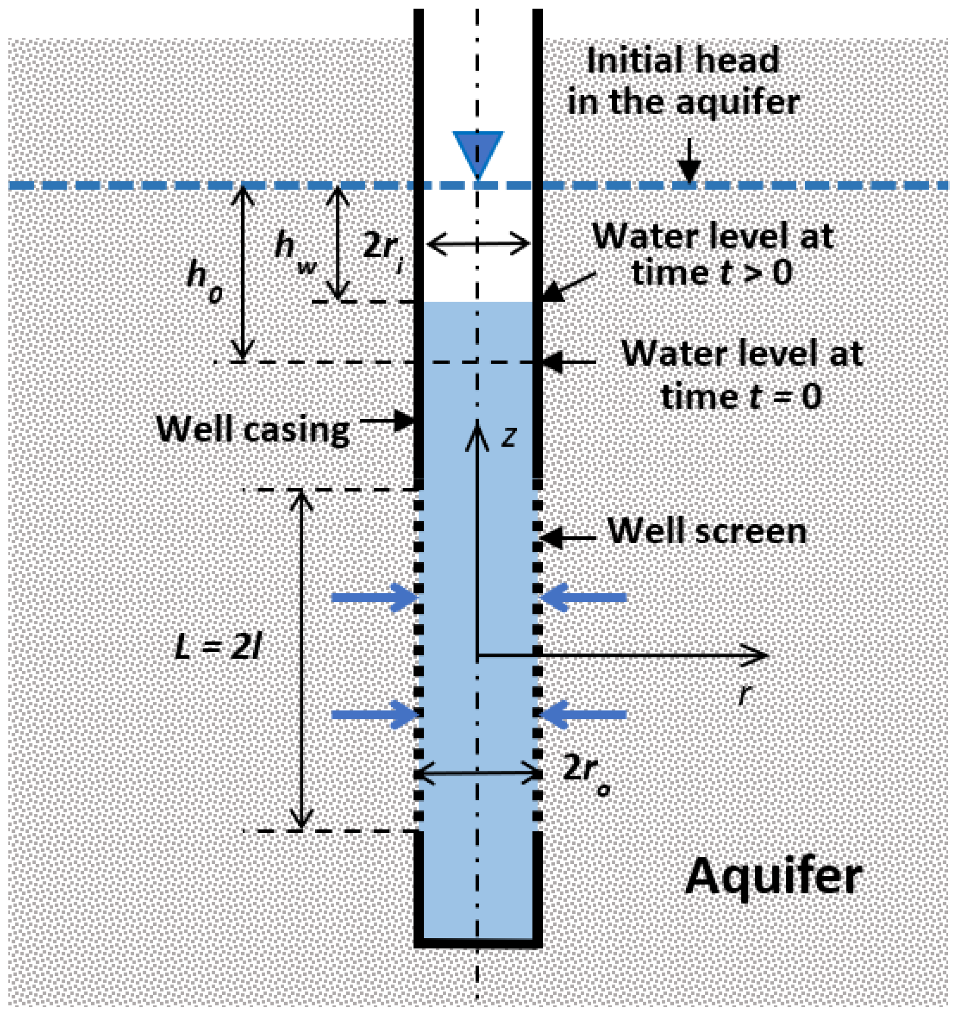
Figure 1.
Schematic diagram of a slug test conducted in a well with a screened section (shown is a rising head test after a small amount of water is extracted from the well at time zero): ri is the inner radius of the well casing, ro is the outer radius of the well screen, L = 2l is the length of the screened section, h0 is the difference in head in the well at time t = 0, hw is the difference in head in the well at time t > 0, and r and z are the radial and vertical coordinates with origin at the center of the screen.

Figure 2.
Plot of the shape factor against the aspect ratio of the well screen obtained with (1) numerical approach given by Equation (18), (2) approximate analytical solution given by Equation (24), (3) Hvorslev approximation [1] given by Equation (3), (4) Bouwer and Rice empirical approach [2], and (5) approximate solution of Zlotnik et al. [13].

Figure 3.
Plot of observed head against time on semilogarithmic paper and slope fitted by linear regression for the falling head slug test performed in Well 4-2, Pratt County Monitoring Site 36, Kansas, U.S [21].
Figure 3.
Plot of observed head against time on semilogarithmic paper and slope fitted by linear regression for the falling head slug test performed in Well 4-2, Pratt County Monitoring Site 36, Kansas, U.S [21].

Figure 4.
Plot of the G-function (Equation (13)) and the approximation for large aspect ratios of the well screen (Equation (20)) against : (a) large-scale general plot; and (b) detailed plot near the origin.
Figure 4.
Plot of the G-function (Equation (13)) and the approximation for large aspect ratios of the well screen (Equation (20)) against : (a) large-scale general plot; and (b) detailed plot near the origin.

Figure 5.
Plot of against derived with the numerical solution, Equation (17) (solid lines), and with the approximate analytical solution, Equation (22) (dotted lines), for aspect ratio equal to 1, 10, and 100.
Figure 5.
Plot of against derived with the numerical solution, Equation (17) (solid lines), and with the approximate analytical solution, Equation (22) (dotted lines), for aspect ratio equal to 1, 10, and 100.


Table 1.
Comparison table for all approaches considered in this study.
| Method | Solution Technique | Flow Distribution at the Well Screen | Aquifer Boundary Conditions |
|---|---|---|---|
| Hvorslev [1] | Analytical | Uniform | No |
| Bouwer and Rice [2] | Empirical | Non-uniform | Yes |
| Zlotnik et al. [13]. | Analytical | Uniform | Yes |
| This study 1 | Numerical | Non-uniform | No |
| This study 2 | Analytical | Non-uniform | No |
Table 2.
Values obtained with the different methods for the shape factor of the slug test and the hydraulic conductivity of the aquifer.
Table 2.
Values obtained with the different methods for the shape factor of the slug test and the hydraulic conductivity of the aquifer.
| Method | Shape Factor | Hydraulic Conductivity K (m/day) |
|---|---|---|
| Numerical, Equations (17) and (18) | 2.25 | 3.67 |
| Analytical, Equation (24) | 2.28 | 3.71 |
| Hvorslev [1], Equation (3) | 2.50 | 4.08 |
| Bouwer and Rice [2] | 2.00 | 3.26 |
| Zlotnik et al. [13] | 2.33 | 3.79 |
Disclaimer/Publisher’s Note: The statements, opinions and data contained in all publications are solely those of the individual author(s) and contributor(s) and not of MDPI and/or the editor(s). MDPI and/or the editor(s) disclaim responsibility for any injury to people or property resulting from any ideas, methods, instructions or products referred to in the content. |
© 2023 by the author. Licensee MDPI, Basel, Switzerland. This article is an open access article distributed under the terms and conditions of the Creative Commons Attribution (CC BY) license (https://creativecommons.org/licenses/by/4.0/).
Share and Cite
MDPI and ACS Style
De Smedt, F. Shape Factor for Analysis of a Slug Test. Water 2023, 15, 2551. https://doi.org/10.3390/w15142551
AMA Style
De Smedt F. Shape Factor for Analysis of a Slug Test. Water. 2023; 15(14):2551. https://doi.org/10.3390/w15142551
Chicago/Turabian StyleDe Smedt, Florimond. 2023. "Shape Factor for Analysis of a Slug Test" Water 15, no. 14: 2551. https://doi.org/10.3390/w15142551
Note that from the first issue of 2016, this journal uses article numbers instead of page numbers. See further details here.