Spatiotemporal Characterization of Drought Magnitude, Severity, and Return Period at Various Time Scales in the Hyderabad Karnataka Region of India

Abstract

Global climate change is anticipated to have a profound impact on drought occurrences, leading to detrimental consequences for the environment, socioeconomic relations, and ecosystem services. In order to evaluate the extent of drought impact, a comprehensive study was conducted in the Hyderabad–Karnataka region, India. Precipitation data from 31 stations spanning a 50-year period (1967–2017) were analyzed using the standardized precipitation index (SPI) based on gamma distribution. The findings reveal that approximately 15% of the assessed years of experienced drought conditions, with a range of influence between 41% and 76% under SPI_3, and between 43% and 72% under SPI_6. Examining the timescale magnitude frequency provided insights into variations in the severity of drought events across different locations and timescales. Notably, the Ballari (−8.77), Chitapur (−8.22), and Aland (−7.40) regions exhibited the most significant magnitudes of drought events for SPI_3 with a 5-year return period. The heightened risk of recurrent droughts in the study area emphasizes the necessity of integrating SPI in decision-making processes, as such integration can markedly contribute to the development of reliable and sustainable long-term water management strategies at regional and national levels.

1. Introduction

The hydrological cycle is profoundly altered by atmospheric circulation patterns driven by climate change [1]. Climate change has substantial impacts on droughts and their spatial distribution, consequently affecting various environmental and socioeconomic factors [2]. Drought can be defined as a prolonged period of abnormally dry weather or water scarcity, resulting in a lack of sufficient water resources to meet the need of a particular region or ecosystem [3]. Droughts, characterized by low precipitation and reduced water availability, have significant impacts on agriculture, ecosystems, and human activities [3,4,5]. They can vary in severity, duration, and spatial extent, causing water shortages, agri-food losses, and an elevated risk of wildfires and ecological imbalances [6,7,8]. However, with the ongoing climate change, the frequency and intensity of droughts are expected to escalate, particularly in arid and semi-arid regions. In addition, it is projected that the global extent affected by extreme droughts, currently ranging from 1% to 3%, will surge to 30% by the 2090s [8]. Furthermore, according to the same source, projections indicate that by 2025, approximately 4 billion people will experience severe water stress, with particularly severe conditions expected in Africa, the Middle East, and South Asia. Such scenarios highlight the urgent need to address the escalating frequency of droughts, as well as accompanying water-related disruptions. Thus, maintaining optimal and more efficient water management has become increasingly challenging and demanding [9,10].

India has witnessed a marked increase in both the frequency and severity of prolonged multi-year droughts in recent decades. Notably, from 1891 to 2009, India experienced 23 large-scale droughts, with their occurrence on the rise [11]. The primary causes of droughts in India are deviations in the total volume and pattern of rainfall during the southwest monsoon, coupled with the effect of rising air temperatures [12,13]. Droughts in the Karnataka state, characterized by spatiotemporal variations in rainfall, reflect the escalating trend of increasing drought severity and frequency observed throughout India [14]. This state exhibits a wide oscillation in rainfall levels, ranging from 4747 mm in the coastal region, 3500 mm in the Malnad region, to as low as 477 mm in the south interior Karnataka. The northern part of Karnataka is particularly susceptible to droughts due to semi-arid climate and low and erratic rainfall patterns, causing both meteorological and hydrological droughts [15]. This region experiences an average annual rainfall of approximately 503 mm, distributed across only 35 rainy days. In this region, the analysis of drought reveals that approximately five droughts with varying degrees of severity occur within a span of ten years. As a result, the region faces challenges due to low rainfall and a short growing season, which typically lasts only 8 to 14 weeks. These factors impose limitations on the choice of crops that can be cultivated in this area. Moreover, insufficient rainfall has a negative impact on replenishing groundwater resources, exacerbating the issue of water scarcity [16]. Thus, understanding the dynamics of droughts in regions like this is crucial for effective water resource management and agricultural resilience.

To evaluate the severity of drought in regions affected by drought, a range of indices have been developed and applied. These indices consider the specific characteristics of the natural hazard, the sectors impacted by drought, and utilize robust scientific approaches and methods [17,18,19]. For instance, the groundwater drought index developed by Goodarzi et al. [20] and the normalized difference vegetation index (NDVI) [21] are two examples of recently developed indices. Brown et al. [22] proposed the vegetation drought response index (VegDRI), which combines NDVI datasets derived from NOAA-AVHRR with climate-based SPI and PDSI drought indices, derived from selected synoptic stations. However, the main drawback of VegDRI is (i) its limited record period due to reliance on remotely sensed data, (ii) it is not applicable outside the vegetation season or during periods when vegetation is minimal. The standardized precipitation index (SPI), developed by Mckee et al. [23], is recognized as the most robust index for analyzing drought severity. Unlike other indices that incorporate additional factors such as the surface water supply index (SWSI), normalized difference vegetation index (NDVI), crop moisture index (CMI), and vegetation condition index (VCI), SPI solely relies on rainfall data. This simplicity and focus on precipitation make SPI highly popular and widely used in drought analysis [13,24,25,26]. For instance, in a study conducted by Spinoni et al. [27], SPI was applied with the standardized precipitation evapotranspiration index (SPEI) and the reconnaissance drought indicator (RDI) in assessing droughts at the EU level. In addition, Meresa et al. [28] studied hydro-meteorological drought in ten Polish catchments by computing SPI, SPEI, and runoff standardized indices for the period of 1971–2100. Thus, the use of SPI can be a valuable approach for water resource management in (agro)ecosystems. The computation of SPI values was considered for the time scales of 3 and 6 months. This will be useful for intermediate and long-term assessments of hydrologic droughts, specifically those affecting, for example, groundwater recharge ability in the country, thus increasing the risk of water shortage [29].

The objective of this study was to enhance our understanding of droughts by analyzing their severity, duration, and frequency, as well as the recurrence intervals at various time scales. In the current study, SPI_3 and SPI_6 were considered because these time scales are often considered relevant for assessing drought in agriculture, as they reflect both short-term fluctuations and longer-term moisture deficits that can affect crop productivity. Furthermore, the application of SPI in this study is deemed essential for sustainable water resource utilization, mitigating the effects of drought on food security and local economies, and adapting to climate change. By incorporating the SPI into decisionmaking, policymakers can formulate resilient and sustainable long-term action plans and strategies for effective water management. The findings from this study can serve as a reliable reference point for the national and/or inter(regional) authorities in identifying drought-prone areas and prioritizing ecological protection measures in the future.

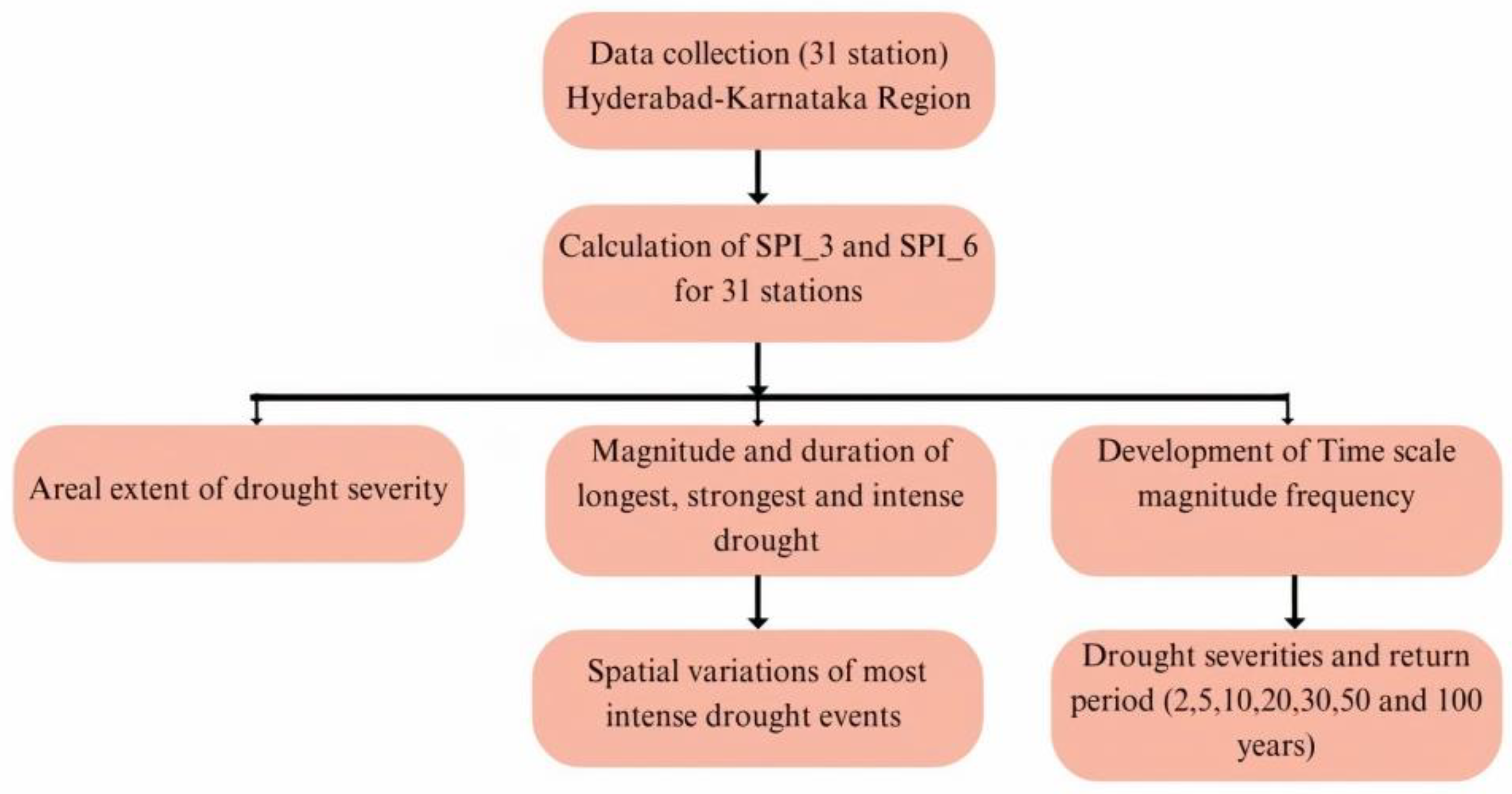
2. Materials and Methods

2.1. Study Area

Hyderabad Karnataka (HK) region is located in the northeastern part of the Karnataka state (14°60′ to 18°30′ N; 75°60′ to 77°70′ E). For this study, a total of 31 stations were considered for drought characterization and modeling. The rainfall data (1967–2017) were collected from the Karnataka State Remote Sensing Applications Centre (KSRSAC) and the Dept. of Economics and Statistics, Bangalore, Karnataka, with the workflow presented in Figure 1.

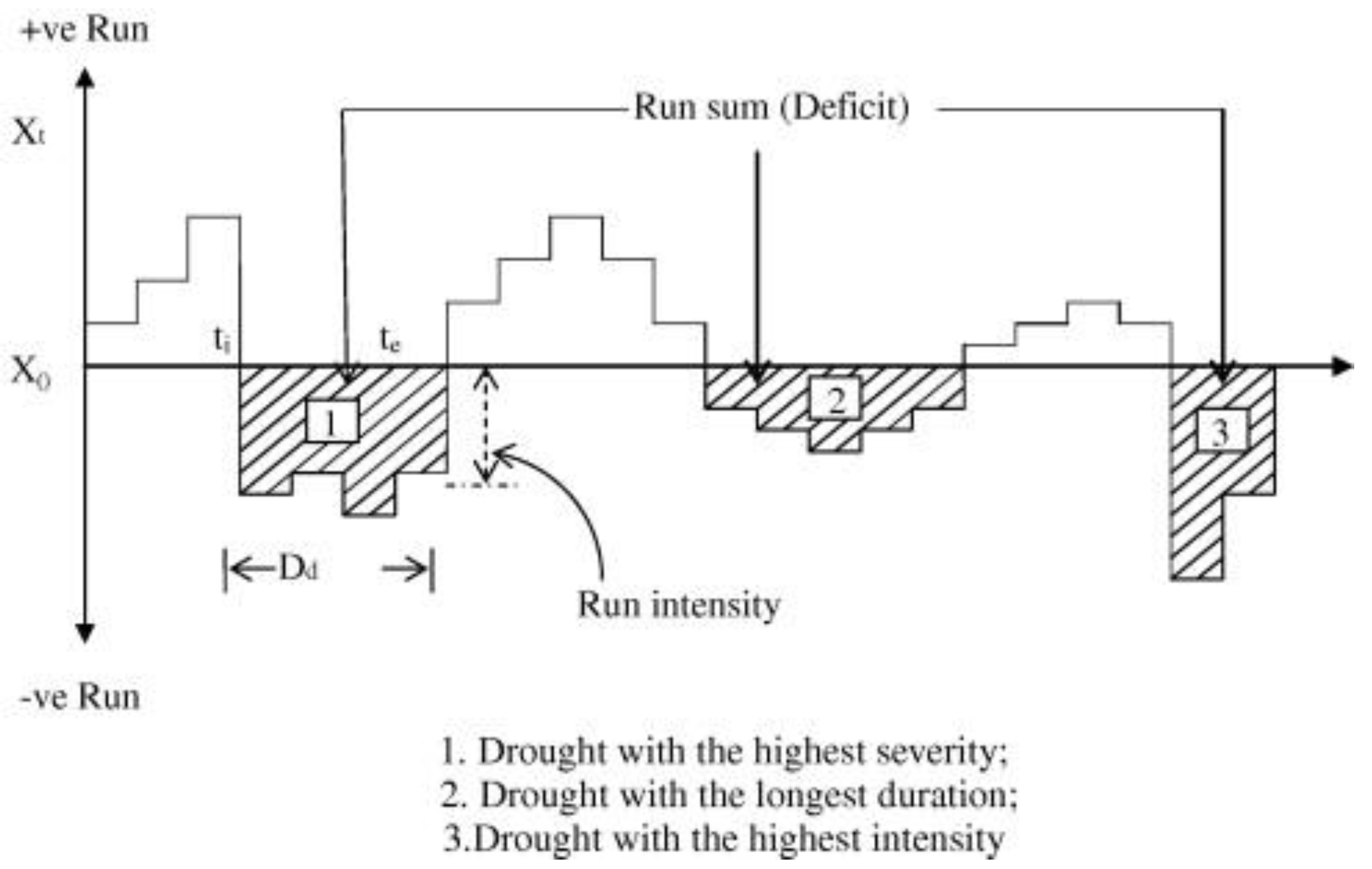
2.2. Standardized Precipitation Index (SPI)

SPI values were determined by fitting the long-term precipitation datato a probability distribution, specifically the Gamma distribution [30,31]. This technique has been applied to rainfall data by Sonmez et al. [32] since the Gamma distribution is well-suited for this type of data.

$$\mathrm{f}(\mathrm{x},\mathsf{\alpha },\mathsf{\beta })=\frac{1}{{\mathsf{\beta }}^{\mathsf{\alpha }}\mathsf{\Gamma }\left(\mathsf{\alpha }\right)}{\mathrm{x}}^{\mathsf{\alpha }-1}{\mathrm{e}}^{-(\frac{\mathrm{x}}{\mathsf{\beta }})} \mathrm{for} \mathrm{x},\mathsf{\alpha },\mathsf{\beta }>0$$

(1)

where α and β represent the shape and scale parameters, respectively; x is the rainfall depth; and Γ(α) is the gamma function. The parametersαand β were estimated using the maximum likelihood method using Equations (2) and (3), respectively.

$$\mathsf{\alpha }=\frac{1}{4\mathrm{A}}\left(1+\sqrt{1+\frac{4\mathrm{A}}{3}}\right)$$

(2)

$$\mathsf{\beta }=\frac{\overline{\mathrm{X}}}{\mathsf{\alpha }}$$

(3)

$$\mathrm{A}=\ln (\overline{\mathrm{X}})-\frac{{\displaystyle \sum _{\mathrm{i}=1}^{\mathrm{n}}\ln \left(\mathrm{x}\right)}}{\mathrm{n}}$$

(4)

Integrating the probability density function (PDF) with respect to x and attach α and β parameters yields the cumulative probability distribution function (CDF) F(x)

$$\mathrm{F}(\mathrm{x},\mathsf{\alpha },\mathsf{\beta })={\displaystyle \underset{0}{\overset{\mathrm{x}}{\int }}\mathrm{f}\left(\mathrm{x},\mathsf{\alpha },\mathsf{\beta }\right)=\frac{1}{{\mathsf{\beta }}^{\mathsf{\alpha }}\mathsf{\Gamma }\left(\mathsf{\alpha }\right)}}{\displaystyle \underset{0}{\overset{\mathrm{x}}{\int }}{\mathrm{x}}^{\mathsf{\alpha }-1}}{\mathrm{e}}^{-\left(\frac{\mathrm{x}}{\mathsf{\beta }}\right)}\mathrm{dx}$$

(5)

which can be expressed by Equation (6)

$$\mathrm{F}(\mathrm{x},\mathsf{\alpha },\mathsf{\beta })=\frac{1}{\mathsf{\Gamma }\left(\mathsf{\alpha }\right)}{\displaystyle \underset{0}{\overset{\mathrm{x}}{\int }}{\mathrm{t}}^{\mathsf{\alpha }-1}}{\mathrm{e}}^{-\mathrm{t}}\mathrm{dx}$$

(6)

where $\mathrm{t}=\frac{\mathrm{x}}{\mathsf{\beta }}$.

Asthegamma function is undefined for x = 0 and the time series of rainfall data may have zero rainfall values, the cumulative probability of zero and non-zero rainfalls, H(x) was calculated using Equation (7).

$$\mathrm{H}\left(\mathrm{x}\right)=\mathrm{q}+(1-\mathrm{q}\left)\mathrm{F}\right(\mathrm{x},\mathsf{\alpha },\mathsf{\beta })$$

(7)

where q represents the probability of zero rainfall events.

The cumulative probability was then transformed into a standardized normal distribution so that mean and variance of SPI are set to 0 and 1, respectively [30].

In order to convert the cumulative probability distribution into a standardized normal distribution, the current study used the approximations offered by [33], which are provided in Equations (8) and (9):

$$\mathrm{SPI}=-\left(\mathrm{k}-\frac{{\mathrm{c}}_0+{\mathrm{c}}_1\mathrm{k}+{\mathrm{c}}_2{\mathrm{k}}^2}{1+{\mathrm{d}}_1\mathrm{k}+{\mathrm{d}}_2{\mathrm{k}}^2+{\mathrm{d}}_3{\mathrm{k}}^3}\right)$$

(8)

$$\mathrm{SPI}=+\left(\mathrm{k}-\frac{{\mathrm{c}}_0+{\mathrm{c}}_1\mathrm{k}+{\mathrm{c}}_2{\mathrm{k}}^2}{1+{\mathrm{d}}_1\mathrm{k}+{\mathrm{d}}_2{\mathrm{k}}^2+{\mathrm{d}}_3{\mathrm{k}}^3}\right)$$

(9)

where

$$\mathrm{k}=\sqrt{\ln \left(\frac{1}{{\left(\mathrm{H}\right(\mathrm{x}\left)\right)}^2}\right)} \mathrm{for} 0<\mathrm{H}\left(\mathrm{x}\right)\le 0.5$$

$$\mathrm{k}=\sqrt{\ln \left(\frac{1}{{(1-\mathrm{H}\left(\mathrm{x}\right))}^2}\right)} \mathrm{for} 0.5<\mathrm{H}\left(\mathrm{x}\right)\le 1$$

C₀ = 2.515517, C₁ = 0.802583, C₂ = 0.010328, d₁ = 1.432788, d₂ = 0.189269 and d₃ = 0.001308.

In this study, SPI values were calculated on a different timescale. The SPI threshold ranges that are used to define drought conditions are presented in

Table 1. Drought classification based on SPI [23].

Drought Classes	SPI
≥2.0	Extremely wet (EW)
1.99 to 1.50	Severe wet (SW)
1.49 to 1.00	Moderately wet (MW)
0.99 to −0.99	Near normal (N)
−1.0 to −1.49	Moderate drought (MD)
−1.50 to −1.99	Severe drought (SD)
≤−2.0	Extreme drought (ED)

.

The regional monthly drought index (DI), derived from mean rainfall data, was used for conducting temporal drought analysis. The run theory was utilized to define drought characteristics such as: the most intense drought (Ie), initiation time (Ti), termination time (Te), duration (Dd), severity (Sd), and intensity (Id) (Figure 2). Yevjevich [34] and Mishra and Singh [11] proposed the use of run theory to define hydrologic drought (Figure 2). The run theory refers to the occurrence of another type of event in the process of continuous occurrence of similar events, such as droughts, continuous rain-free days, rainy days, alternating natural water occurrence, etc. [35].

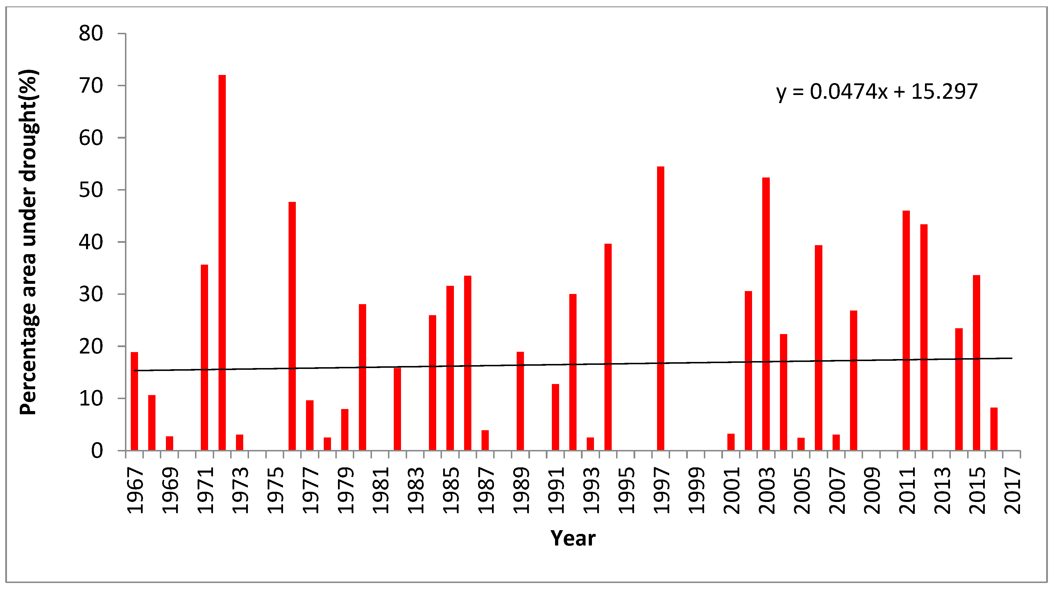
2.3. Areal Extent of Drought Severity at Different Timescales

The study area was bifurcated using the Thiessen Polygon [36] tool in ArcGIS v. 10.2.2 software into 31 polygons, corresponding to 31 rain gauge stations. Each polygon in the study area represents the spatial extent of influence of a rain gauge station, measured in square kilometers and expressed as a fraction of the total study area. The timescale of 3 (SPI_3) and 6 (SPI_6) months were selected for the determination of areal drought events.

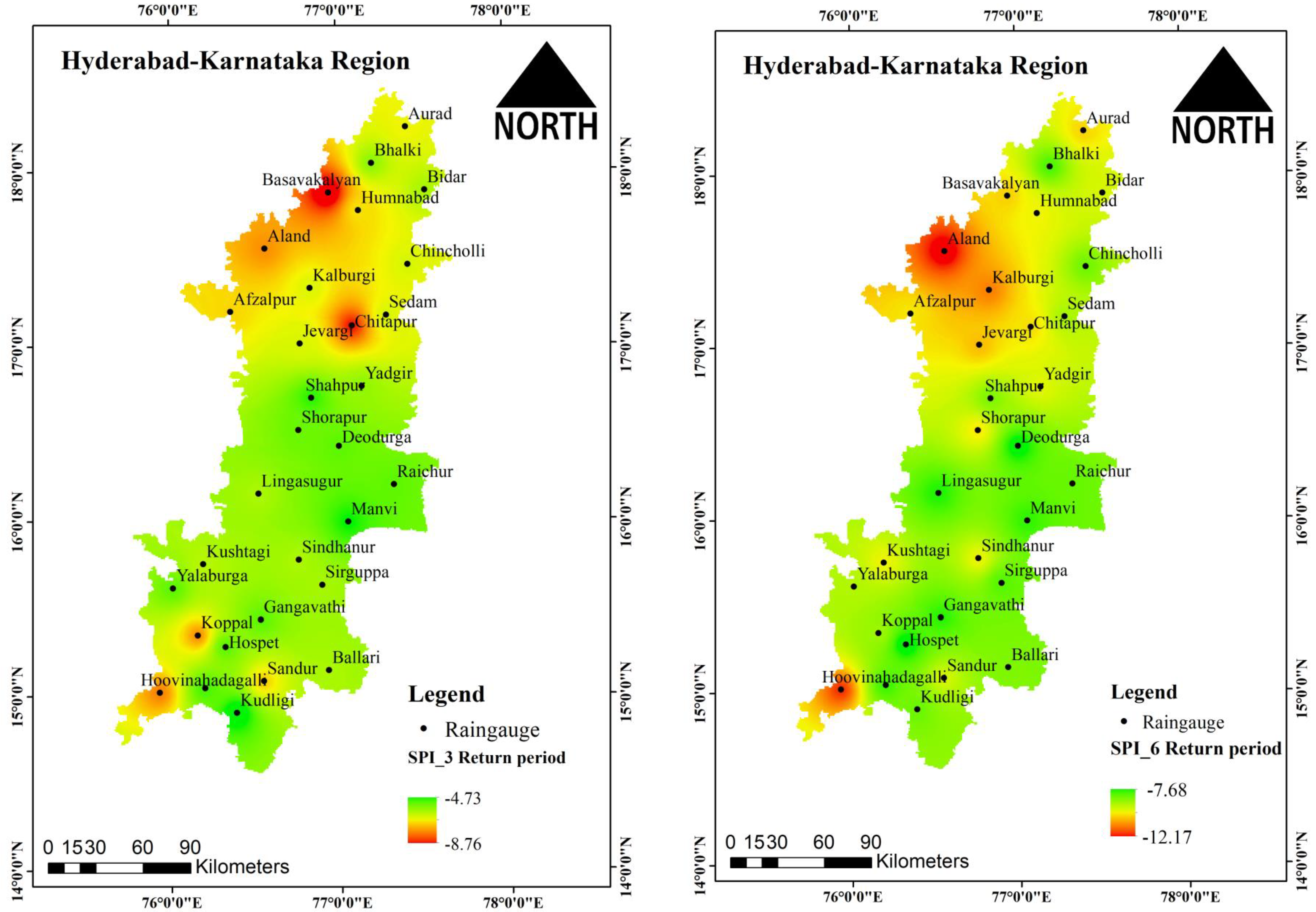
2.4. Spatial Drought Analysis

Spatial analysis of drought was conducted using station DI values derived from monthly rainfall data (SPI_3 and SPI_6) within the same ArcGIS interface, employing the inverse distance weighing (IDW) technique to spatially visualize drought values over the study area. A similar approach was applied by Subedi et al. [37] in studying spatio-temporal changes during a drought in Texas, USA, based on the SPEI index. The general form of the IDW approach [38] is given by:

$${\mathrm{Z}}_{\mathrm{ni}}=\frac{{\displaystyle \sum _{\mathrm{j}=1}^{\mathrm{m}}\left(\frac{{\mathrm{z}}_{\mathrm{j}}}{{\mathrm{d}}_{\mathrm{j}}^{\mathrm{p}}}\right)}}{{\displaystyle \sum _{\mathrm{j}=1}^{\mathrm{m}}\left(\frac{1}{{\mathrm{d}}_{\mathrm{j}}^{\mathrm{p}}}\right)}}$$

(10)

Z_ni represents the new value for given grid j; Z_j represents the value of the m nearest neighbors; d_j represents the distance to m—nearest neighbors; p is the exponent of distance, whereas the exponent of distance was set as 2 for spatial interpolation of DI values.

2.5. Development of Time Scale Magnitude Frequency (TMF)

In order to describe the statistical characteristics of droughts in the study area, a thorough review was conducted to select an appropriate theoretical distribution function, ultimately choosing the Extreme Value type 1 (EV1) distribution function [39]. The EV1 was selected because (i) it is easy to apply as a two-parameter frequency distribution function, and (ii) visual inspection of EV1vs. other frequency distribution functions (the generalized extreme value—GEV, the three-parameter lognormal distribution—LN3 or the Log-Pearson distribution—LP3) suggests that EV1 gives more accurate estimation for dry and wet periods [40,41]. The next step involved fitting and testing the distribution function against the cumulative severity values of the DI at different time scales by using next equations:

$$\mathrm{F}\left(\mathrm{x}\right)=\exp (-\exp (-\mathsf{\alpha }(\mathrm{x}-\mathsf{\mu }\left)\right))$$

(11)

where

• α = Shape parameter
• u = Location parameter

These parameters were determined from the relations:

$$\mathsf{\alpha }=\frac{1.283}{\mathsf{\sigma }}$$

(12)

$$\mathrm{u}=\overline{\mathrm{x}}+\mathrm{K}\mathsf{\sigma }$$

(13)

• $\overline{\mathrm{x}}$ = mean
• $\mathsf{\sigma }$ = standard deviation

$$\mathrm{K}=-0.78\left. [0.577+\left(\ln \left(\ln \frac{\mathrm{T}}{\mathrm{T}-1}\right)\right)\right]$$

(14)

where

• T = return period (years) of the event of a defined duration.

Based on Equation (14) [41] the drought severities corresponding to selected return periods of 2, 5, 10, 20, 30, 50 and 100 years were computed for each event.

3. Results and Discussion

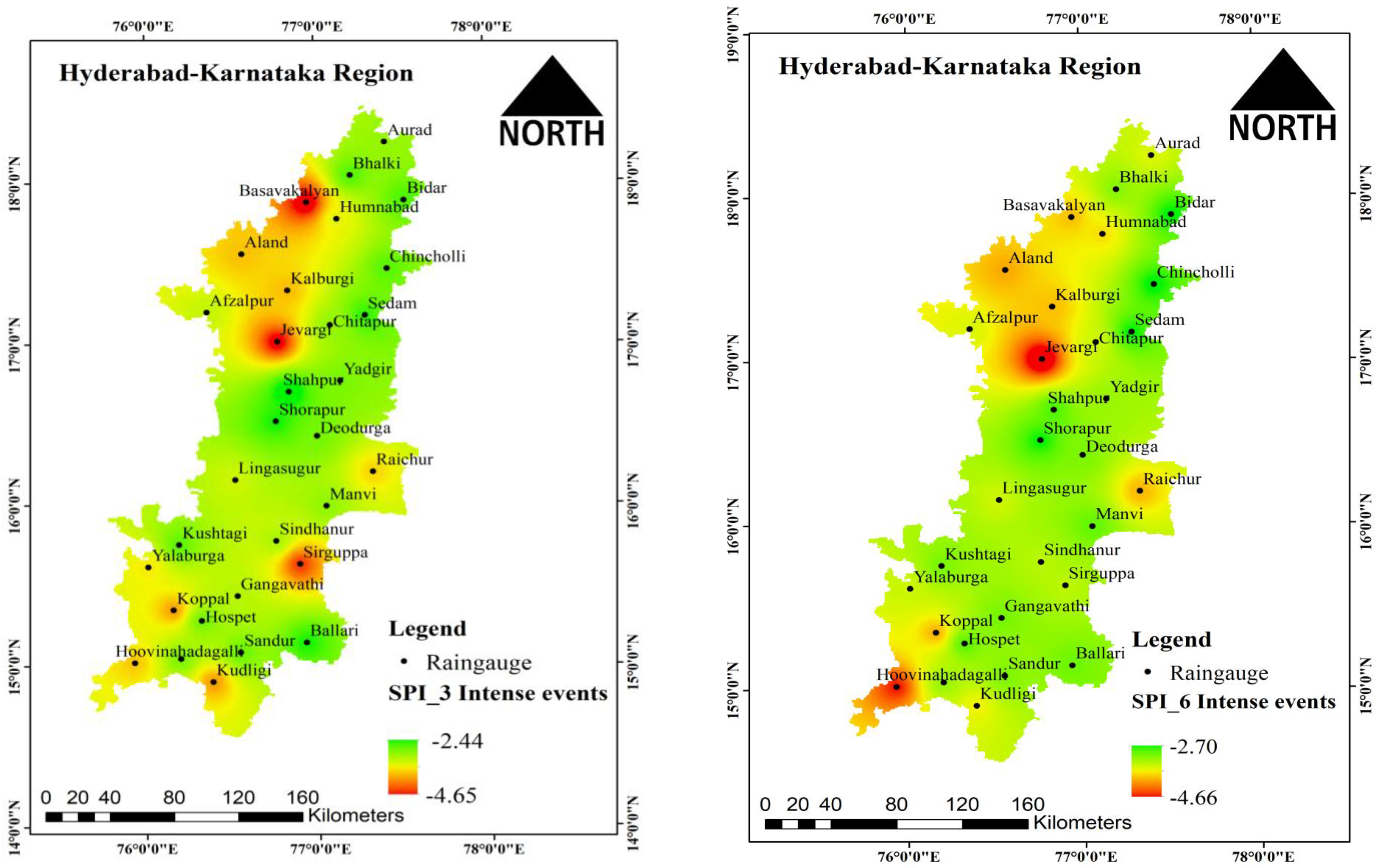
3.1. Spatiotemporal Variation of Drought Events

Figure 3 illustrates the spatial distribution of the most severe droughts across different timescales. For the SPI_3 timescales, the longest drought event occurred during 1992 (April–December) and 1984–1985 (May–January) in Jeevargi and Aland, lasting 9 months with severity values of −21.68 and −14.33, respectively. Furthermore, an intense drought event was observed in Ballari in June 2003, with a severity value of −4.66 (Table 2). Regarding the SPI_6 timescales, the longest events were identified as 1984–1985 (June–September) and 1991–1993 (December–March) in Aland and Jeevargi, lasting 16 months with a severity value of −29.38 and −43.48, respectively. Additionally, an intense drought event was recorded in February 1993 in Jeevargi under SPI_6, with a severity value of −4.67 (Table 3). It is crucial to effectively utilize this information to address the challenges posed by drought disasters.

Based on a 48-year analysis (1961 to 2008), it was found that significant areas of the district faced severe drought conditions in 1972 and 2003 [42]. In the Bellary region, SPI_1, SPI_6, and SPI_12 were employed as drought indicators, indicating the occurrence of moderate, severe, and extreme droughts at a high frequency [43]. For SPEI-1, the highest intensity that occurred in geophysics station Lembang –Bandung about −2.931 in October 2012 with a value of severity −2.931 with a month duration. And thehighest intensity for SPEI-3 was recorded in meteorology station Selaparang–Mataram about −2.485 with severity −7.455 and duration of 3 months occurred in June–August 2009 [44].

Table 2. Magnitude and duration of the longest, strongest, and intense drought events in HK region using SPI_3 [44].

Station	Longest		Strongest		Highest
	Year	D	Year	S	Year	I
Afzalpur	1972 (June–November)	6	1972 (June–November)	−13.33	1976 (June)	−3.28
Aland	1984–1985 (May–January)	9	1984–1985 (May–January)	−14.33	2003 (December)	−3.75
Aurad	1980 (July–December)	6	1980 (July–December)	−8.13	1966 (July)	−3.08
Ballari	1976 (May–December)	8	1976 (May–December)	−14.55	2003 (June)	−4.66
Basavakalyan	1972 (July–October)	6	1972 (July–October)	−10.98	1984 (July)	−2.65
Bhalki	1972 (July–November)	2	1972 (July–November)	−10.93	1972 (September)	−2.8
Bidar	1979 (April–August)	5	1979 (April–August)	−7.36	1972 (August)	−2.78
Chincholli	1971 (June–November)	6	1971 (June–November)	−11.54	1972 (September)	−2.83
Chitapur	1972 (May–December)	8	1972 (May–December)	−15.5	1994 (July)	−3.07
Deodurga	1971 (June–September)	4	1972 (September–November)	−7.23	2011 (November)	−2.94
Gangavathi	2016 (October–December)	3	2016 (October–December)	−6.88	2003 (June)	−3.22
Hoovinahadagali	1965 (April–July), 2002 (August–November) and 2008 (June–September)	4	2008 (June–September)	−7.24	1976 (October)	−2.96
Hagaribommanahalli	2003 (May–November)	7	2003 (May–November)	−14.72	2003 (July)	−3.72
Hospet	2001 (April–July), 2004 (September–December) and 2016 (September–December)	4	2016 (September–December)	−8.59	2016 (December)	−2.92
Humnabad	2001 (March–August)	6	2001 (March–August)	−10.68	1965 (May)	−3.47
Jeewargi	1992 (April–December)	9	1992 (April–December)	−21.68	1992 (November)	−4.55
Kalburgi	1972 (July–October)	4	1972 (July–October)	−10.06	1965 (June)	−3.77
Koppal	2003 (May–September) and 2016 (August–December)	5	2003 (May–September)	−11.35	2003 (July)	−3.9
Kudligi	1970 (June–November)	6	1970 (June–November)	−12.51	1976 (July)	−3.92
Kustigi	2003 (May–November)	7	2003 (May–November)	−12.69	2011 (November)	−2.85
Lingasugur	2001 (May–August)	4	2014 (May–July)	−8.03	2014 (June)	−3.34
Manvi	1994 (June–September)	4	1994 (June–September)	−7.25	2015 (July)	−3.06
Raichur	1994 (May–September)	5	1994 (May–September)	−10.49	2011 (November)	−3.67
Sandur	1976 (June–December)	7	1976 (June–December)	−10.68	2003 (July)	−2.89
Sedam	1972 (July–December)	6	1972 (July–December)	−10.96	1979 (August)	−2.71
Shahpur	1992 (Junee–October) and 1994 (May–September)	5	1994 (May–September)	−8.31	1972 (August)	−2.44
Shorapur	1986 (July–November)	5	1986 (July–November)	−7.5	2011 (November)	−2.64
Sindhanur	1997 (June–October)	5	2006 (August–November)	−7.97	1989 (May)	−3.18
Sirguppa	1972 (August–December)	5	1972 (August–December)	−6.37	2008 (June)	−4.31
Yadgir	1971 (July–November), 2014(April–August) and 2015(June–October)	5	2014 (April–August)	−9.61	2015 (August)	−2.96
Yalburga	1985 (September–December), 1991 (September–December) and 2001 (May–August)	4	2001 (May–August)	−8.08	1984 (June)	−3.58

Table 2. Magnitude and duration of the longest, strongest, and intense drought events in HK region using SPI_3 [44].

Station	Longest		Strongest		Highest
	Year	D	Year	S	Year	I
Afzalpur	1972 (June–November)	6	1972 (June–November)	−13.33	1976 (June)	−3.28
Aland	1984–1985 (May–January)	9	1984–1985 (May–January)	−14.33	2003 (December)	−3.75
Aurad	1980 (July–December)	6	1980 (July–December)	−8.13	1966 (July)	−3.08
Ballari	1976 (May–December)	8	1976 (May–December)	−14.55	2003 (June)	−4.66
Basavakalyan	1972 (July–October)	6	1972 (July–October)	−10.98	1984 (July)	−2.65
Bhalki	1972 (July–November)	2	1972 (July–November)	−10.93	1972 (September)	−2.8
Bidar	1979 (April–August)	5	1979 (April–August)	−7.36	1972 (August)	−2.78
Chincholli	1971 (June–November)	6	1971 (June–November)	−11.54	1972 (September)	−2.83
Chitapur	1972 (May–December)	8	1972 (May–December)	−15.5	1994 (July)	−3.07
Deodurga	1971 (June–September)	4	1972 (September–November)	−7.23	2011 (November)	−2.94
Gangavathi	2016 (October–December)	3	2016 (October–December)	−6.88	2003 (June)	−3.22
Hoovinahadagali	1965 (April–July), 2002 (August–November) and 2008 (June–September)	4	2008 (June–September)	−7.24	1976 (October)	−2.96
Hagaribommanahalli	2003 (May–November)	7	2003 (May–November)	−14.72	2003 (July)	−3.72
Hospet	2001 (April–July), 2004 (September–December) and 2016 (September–December)	4	2016 (September–December)	−8.59	2016 (December)	−2.92
Humnabad	2001 (March–August)	6	2001 (March–August)	−10.68	1965 (May)	−3.47
Jeewargi	1992 (April–December)	9	1992 (April–December)	−21.68	1992 (November)	−4.55
Kalburgi	1972 (July–October)	4	1972 (July–October)	−10.06	1965 (June)	−3.77
Koppal	2003 (May–September) and 2016 (August–December)	5	2003 (May–September)	−11.35	2003 (July)	−3.9
Kudligi	1970 (June–November)	6	1970 (June–November)	−12.51	1976 (July)	−3.92
Kustigi	2003 (May–November)	7	2003 (May–November)	−12.69	2011 (November)	−2.85
Lingasugur	2001 (May–August)	4	2014 (May–July)	−8.03	2014 (June)	−3.34
Manvi	1994 (June–September)	4	1994 (June–September)	−7.25	2015 (July)	−3.06
Raichur	1994 (May–September)	5	1994 (May–September)	−10.49	2011 (November)	−3.67
Sandur	1976 (June–December)	7	1976 (June–December)	−10.68	2003 (July)	−2.89
Sedam	1972 (July–December)	6	1972 (July–December)	−10.96	1979 (August)	−2.71
Shahpur	1992 (Junee–October) and 1994 (May–September)	5	1994 (May–September)	−8.31	1972 (August)	−2.44
Shorapur	1986 (July–November)	5	1986 (July–November)	−7.5	2011 (November)	−2.64
Sindhanur	1997 (June–October)	5	2006 (August–November)	−7.97	1989 (May)	−3.18
Sirguppa	1972 (August–December)	5	1972 (August–December)	−6.37	2008 (June)	−4.31
Yadgir	1971 (July–November), 2014(April–August) and 2015(June–October)	5	2014 (April–August)	−9.61	2015 (August)	−2.96
Yalburga	1985 (September–December), 1991 (September–December) and 2001 (May–August)	4	2001 (May–August)	−8.08	1984 (June)	−3.58

Table 3. Magnitude and duration of the longest, strongest and intense drought events in HK region using SPI_6 [44].

Station	Longest		Strongest		Highest
	Year	D	Year	S	Year	I
Afzalpur	1972–1973 (April–March)	12	1972–1973 (April–March)	−27.64	1972 (October)	−3.4
Aland	1984–1985 (June–September)	16	1984–1985 (June–September)	−29.38	2004 (March)	−3.81
Aurad	1965–1966 (October–August)	11	1965–1966 (October–August)	−20.21	1971 (March)	−3.41
Ballari	1976–1977 (May–March)	11	1976–1977 (May–March)	−25.25	2003 (September)	−3.72
Basavakalyan	1972–1973 (July–March)	9	1972–1973 (July–March)	−20.02	1972 (December)	−2.98
Bhalki	1972–1973 (July–February)	8	1972–1973 (July–February)	−20.14	1972 (October)	−3.08
Bidar	1971 (March–December)	10	1972–1973(June–Jan)	−17.15	1972(October)	−2.71
Chincholli	1971–1972 (January–February)	9	1971–1972 (January–February)	−19.57	1971 (September)	−2.7
Chitapur	1972–1973 (June–March)	10	1972–1973 (June–March)	−24.7	1972 (August)	−3.36
Deodurga	1972–1973 (August–February)	7	1972–1973 (August–February)	−13.7	1971 (July)	−3.03
Gangavathi	1972 (June–Jan)	8	1972 (June–Jan)	−13.29	1963 (July)	−3
Hoovinahadagalli	2002–2003 (August–March) and 2003 (May–December)	8	2003 (May–December)	−15.57	2000 (May)	−3.13
Hagaribommanahalli	2003–2004 (April–February)	11	2003–2004 (April–February)	−27.45	2003 (July)	−4.3
Hospet	1997 (May–November)	7	1997 (May–November)	−12.13	2017 (March)	−2.91
Humnabad	1972–1973 (June–February)	9	1972–1973 (June–February)	−21.59	1965 (May)	−3.61
Jeewargi	1991–1993 (December–March)	16	1991–1993 (December–March)	−43.48	1993 (February)	−4.67
Kalburgi	1972–1973 (July–March)	9	1972–1973 (July–March)	−21.61	1965 (June)	−3.73
Koppal	2016–2017 (August–March)	8	2003 (May–November)	−15.86	2003 (July)	−3.78
Kudligi	1976–1977 (June–February)	9	1976–1977 (June–February)	−19.81	1990 (March)	−3.51
Kustigi	1985–1988 (June–March)	10	1985–1988 (June–March)	−21.35	2017 (March)	−3.02
Lingasugur	2011–2012 (October–April)	7	2011–2012 (October–April)	−11.96	2014 (June)	−3.36
Manvi	2002 (April–November)	8	1994 (June–November)	−11.23	1994 (September)	−2.94
Raichur	2012–2013 (May–June)	9	2012–2013 (May–June)	−15.4	2012 (February)	−3.76
Sandur	1976–1977 (June–March)	10	1976–1977 (June–March)	−19.08	2003 (July)	−3.03
Sedam	1972–1973 (July–March)	9	1972–1973 (July–March)	−20.06	1972 (December)	−2.72
Shahpur	2002–2003 (June–Jan), 2000–2004 (September–April) and 2014 (April–November)	9	2014 (April–November)	−15.37	2016 (March)	−2.87
Shorapur	1967–1968 (May–March)	11	1967–1968 (May–March)	−17.48	2012 (February)	−2.72
Sindhanur	2016–2017 (November–August)	10	2016–2017 (November–August)	−19.59	1989 (May)	−3.27
Sirguppa	2002–2003 (June–Jan)	8	2002–2003 (June–Jan)	−17.12	2002 (September)	−3.28
Yadgir	2014 (April–December)	9	2014 (April–December)	−17.38	1981 (March)	−3.14
Yalburga	2012–2013 (May–February)	10	2012–2013 (May–February)	−15.26	2001 (July)	−3.35

Table 3. Magnitude and duration of the longest, strongest and intense drought events in HK region using SPI_6 [44].

Station	Longest		Strongest		Highest
	Year	D	Year	S	Year	I
Afzalpur	1972–1973 (April–March)	12	1972–1973 (April–March)	−27.64	1972 (October)	−3.4
Aland	1984–1985 (June–September)	16	1984–1985 (June–September)	−29.38	2004 (March)	−3.81
Aurad	1965–1966 (October–August)	11	1965–1966 (October–August)	−20.21	1971 (March)	−3.41
Ballari	1976–1977 (May–March)	11	1976–1977 (May–March)	−25.25	2003 (September)	−3.72
Basavakalyan	1972–1973 (July–March)	9	1972–1973 (July–March)	−20.02	1972 (December)	−2.98
Bhalki	1972–1973 (July–February)	8	1972–1973 (July–February)	−20.14	1972 (October)	−3.08
Bidar	1971 (March–December)	10	1972–1973(June–Jan)	−17.15	1972(October)	−2.71
Chincholli	1971–1972 (January–February)	9	1971–1972 (January–February)	−19.57	1971 (September)	−2.7
Chitapur	1972–1973 (June–March)	10	1972–1973 (June–March)	−24.7	1972 (August)	−3.36
Deodurga	1972–1973 (August–February)	7	1972–1973 (August–February)	−13.7	1971 (July)	−3.03
Gangavathi	1972 (June–Jan)	8	1972 (June–Jan)	−13.29	1963 (July)	−3
Hoovinahadagalli	2002–2003 (August–March) and 2003 (May–December)	8	2003 (May–December)	−15.57	2000 (May)	−3.13
Hagaribommanahalli	2003–2004 (April–February)	11	2003–2004 (April–February)	−27.45	2003 (July)	−4.3
Hospet	1997 (May–November)	7	1997 (May–November)	−12.13	2017 (March)	−2.91
Humnabad	1972–1973 (June–February)	9	1972–1973 (June–February)	−21.59	1965 (May)	−3.61
Jeewargi	1991–1993 (December–March)	16	1991–1993 (December–March)	−43.48	1993 (February)	−4.67
Kalburgi	1972–1973 (July–March)	9	1972–1973 (July–March)	−21.61	1965 (June)	−3.73
Koppal	2016–2017 (August–March)	8	2003 (May–November)	−15.86	2003 (July)	−3.78
Kudligi	1976–1977 (June–February)	9	1976–1977 (June–February)	−19.81	1990 (March)	−3.51
Kustigi	1985–1988 (June–March)	10	1985–1988 (June–March)	−21.35	2017 (March)	−3.02
Lingasugur	2011–2012 (October–April)	7	2011–2012 (October–April)	−11.96	2014 (June)	−3.36
Manvi	2002 (April–November)	8	1994 (June–November)	−11.23	1994 (September)	−2.94
Raichur	2012–2013 (May–June)	9	2012–2013 (May–June)	−15.4	2012 (February)	−3.76
Sandur	1976–1977 (June–March)	10	1976–1977 (June–March)	−19.08	2003 (July)	−3.03
Sedam	1972–1973 (July–March)	9	1972–1973 (July–March)	−20.06	1972 (December)	−2.72
Shahpur	2002–2003 (June–Jan), 2000–2004 (September–April) and 2014 (April–November)	9	2014 (April–November)	−15.37	2016 (March)	−2.87
Shorapur	1967–1968 (May–March)	11	1967–1968 (May–March)	−17.48	2012 (February)	−2.72
Sindhanur	2016–2017 (November–August)	10	2016–2017 (November–August)	−19.59	1989 (May)	−3.27
Sirguppa	2002–2003 (June–Jan)	8	2002–2003 (June–Jan)	−17.12	2002 (September)	−3.28
Yadgir	2014 (April–December)	9	2014 (April–December)	−17.38	1981 (March)	−3.14
Yalburga	2012–2013 (May–February)	10	2012–2013 (May–February)	−15.26	2001 (July)	−3.35

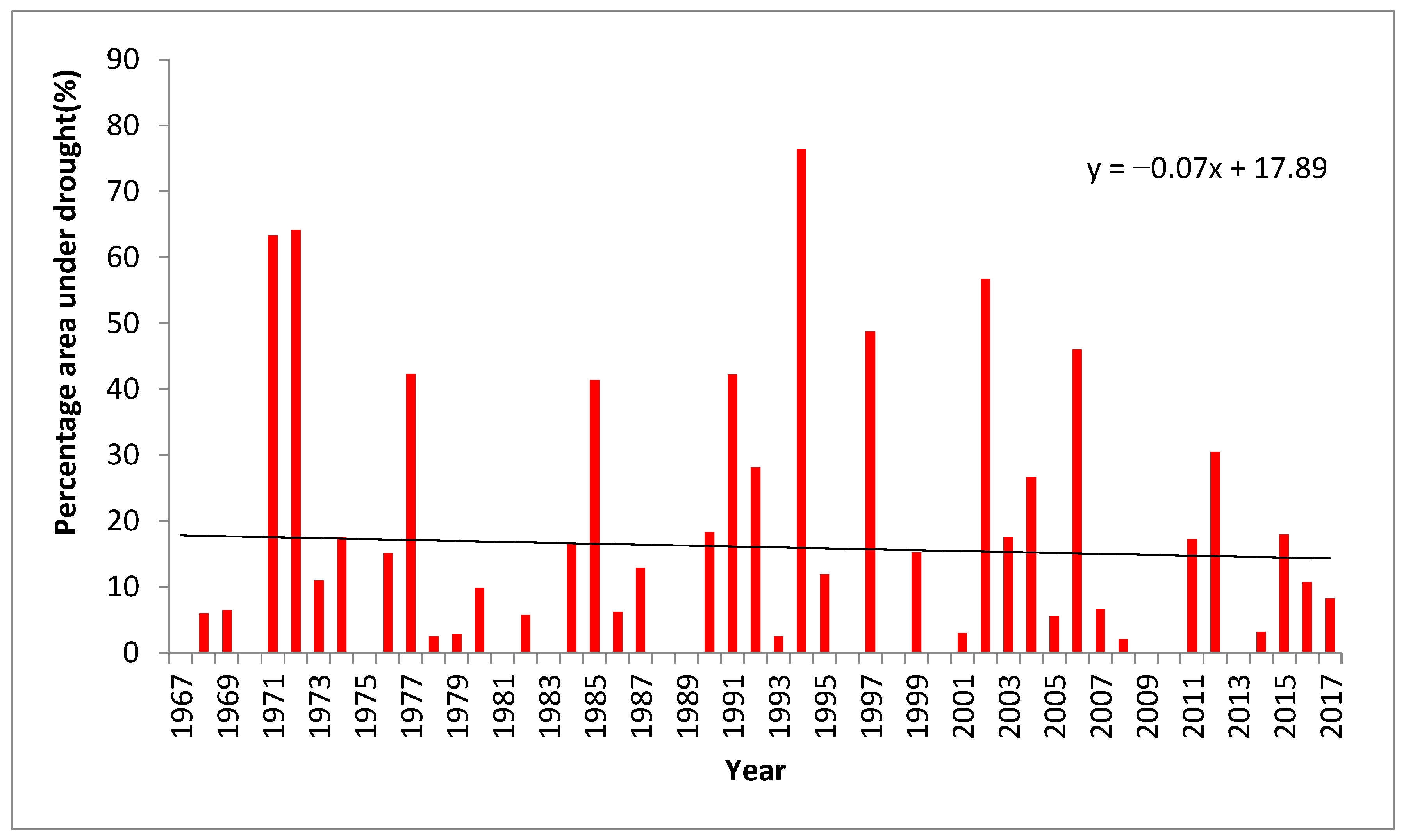
3.2. Areal Extent of Drought Severity in the Hyderabad Karnataka Region Based on Different Timescales

To assess the spatial extent of drought, the study area was examined using SPI_3 for September (Figure 4) and SPI_6 for October (Figure 5). There was no significant trend in the drought area over time period, as the fitted lines in Figure 4 and Figure 5 are straight with no significant slope. The Thiessen polygon method, employed in ArcGIS was also used by Wambua et al. [45] across drought-affected areas in the central highland region of Vietnam to determine contributing areas of each rain gauge station. The analysis of the areal extent of drought under SPI_3 for September (Figure 4) confirmed that drought has impacted more than 41 percent of the study area during the years 1971, 1972, 1977, 1985, 1991, 1994, 1997, 2002, and 2006 with percentages of 63.33, 64.12, 42.34, 41.41, 42.45, 76.40, 48.73, 56.75, and 46.02, respectively. Such results indicate that approximately 15 percent of the examined period experienced agricultural drought, encompassing an area of more than 40 percent under SPI_3 September. Additionally, the years 1971, 1972 and 1994 were particularly critical, with an area of influence exceeding 60 percent. Overall, 1994 was identified as the year with the highest drought impact (Figure 4).

Based on the analysis of the areal extent of drought under SPI_6 for October (Figure 5), it was observed that during 1972, 1976, 1997, 2003, 2011, and 2012, drought conditions affected more than 40 percent of the examined area, with percentages ranging from 43.38 to 72.01. Throughout the entire study period, 1972 emerged as the year with the most severe drought conditions (Figure 5). There was no significant trend in the drought area over time period, as the fitted lines in Figure 4 and Figure 5 are straight with no significant slope.

3.3. Timescale–Magnitude–Frequency (TMF) for Different Timescales in the Hyderabad–Karnataka Region

The historical record of droughts for each rain gauge station and different timescales were identified and tabulated based on the computed SPI time series. These successive drought events were summed up annually and fitted to Extreme value type-I (EV1) distribution. Return periods at various intervals, including 2, 5, 10, 20, 30, 50, and 100 years, were estimated for all 31 stations after fitting the data to EV1 (

Table 4. Severity and return periodfor SPI_3 and SPI_6 timescalesover the Hyderabad–Karnataka region.

Stations	Return Period (SPI_3)							Return Period (SPI_6)
	2	5	10	20	30	50	100	2	5	10	20	30	50	100
Afzalpur	−4.33	−6.88	−8.56	−10.18	−11.11	−12.28	−13.85	−4.88	−10.05	−13.47	−16.76	−18.64	−21.00	−24.19
Aland	−4.55	−7.40	−9.29	−11.10	−12.14	−13.45	−15.20	−6.02	−12.18	−16.26	−20.18	−22.43	−25.24	−29.04
Aurad	−4.52	−6.59	−7.96	−9.27	−10.03	−10.98	−12.25	−5.68	−10.21	−13.20	−16.07	−17.72	−19.79	−22.57
Ballari	−5.24	−8.77	−11.11	−13.36	−14.65	−16.26	−18.44	−5.89	−10.26	−13.16	−15.94	−17.54	−19.54	−22.24
Basavakalyan	−4.12	−5.99	−7.23	−8.42	−9.10	−9.96	−11.11	−4.82	−8.71	−11.29	−13.76	−15.18	−16.96	−19.36
Bhalki	−3.90	−5.79	−7.04	−8.24	−8.93	−9.80	−10.96	−4.62	−8.29	−10.72	−13.06	−14.40	−16.07	−18.34
Bidar	−4.11	−6.01	−7.28	−8.49	−9.19	−10.06	−11.23	−5.88	−9.57	−12.01	−14.35	−15.70	−17.38	−19.65
Chincholli	−4.19	−6.37	−7.82	−9.20	−10.00	−10.99	−12.33	−4.75	−8.59	−11.13	−13.57	−14.97	−16.73	−19.09
Chitapur	−5.13	−8.22	−10.26	−12.22	−13.35	−14.76	−16.66	−5.23	−10.13	−13.37	−16.49	−18.28	−20.51	−23.53
Deodurga	−4.09	−5.43	−6.32	−7.17	−7.66	−8.27	−9.09	−4.90	−7.77	−9.68	−11.50	−12.55	−13.87	−15.64
Gangavathi	−4.24	−5.44	−6.23	−7.00	−7.43	−7.98	−8.72	−5.23	−8.09	−9.98	−11.80	−12.84	−14.15	−15.91
Hoovinahadagalli	−3.88	−5.28	−6.21	−7.10	−7.61	−8.25	−9.11	−5.07	−8.18	−10.24	−12.21	−13.35	−14.77	−16.68
Hagaribommanahalli	−4.70	−7.52	−9.40	−11.19	−12.22	−13.52	−15.26	−6.22	−11.67	−15.28	−18.75	−20.74	−23.23	−26.59
Hospet	−3.95	−5.43	−6.41	−7.36	−7.90	−8.58	−9.49	−4.89	−7.68	−9.52	−11.29	−12.31	−13.58	−15.29
Humnabad	−4.46	−6.79	−8.34	−9.82	−10.67	−11.74	−13.18	−5.63	−9.87	−12.67	−15.36	−16.91	−18.84	−21.45
Jevargi	−4.11	−6.39	−7.89	−9.34	−10.17	−11.21	−12.61	−5.42	−10.44	−13.77	−16.96	−18.79	−21.09	−24.18
Kalburgi	−4.46	−6.42	−7.71	−8.96	−9.67	−10.57	−11.77	−5.96	−11.01	−14.35	−17.56	−19.40	−21.71	−24.82
Koppal	−5.17	−7.41	−8.89	−10.31	−11.12	−12.15	−13.52	−5.41	−9.01	−11.39	−13.68	−15.00	−16.64	−18.86
Kudligi	−3.43	−4.73	−5.60	−6.43	−6.91	−7.50	−8.31	−4.99	−8.56	−10.92	−13.18	−14.48	−16.11	−18.31
Kustigi	−4.02	−6.12	−7.52	−8.86	−9.63	−10.59	−11.89	−5.63	−9.84	−12.62	−15.28	−16.82	−18.74	−21.33
Lingasugur	−4.53	−6.02	−7.02	−7.97	−8.51	−9.20	−10.12	−5.11	−8.03	−9.97	−11.82	−12.89	−14.23	−16.03
Manvi	−3.68	−5.04	−5.94	−6.80	−7.30	−7.92	−8.76	−5.66	−8.13	−9.76	−11.33	−12.23	−13.36	−14.88
Raichur	−3.60	−5.45	−6.67	−7.85	−8.53	−9.37	−10.51	−5.08	−8.50	−10.76	−12.93	−14.17	−15.73	−17.84
Sandur	−4.36	−6.93	−8.63	−10.26	−11.20	−12.37	−13.96	−4.88	−9.57	−12.67	−15.65	−17.36	−19.50	−22.38
Sedam	−4.57	−6.38	−7.58	−8.74	−9.40	−10.23	−11.35	−5.38	−9.12	−11.59	−13.97	−15.33	−17.04	−19.34
Shahpur	−3.74	−5.16	−6.09	−6.99	−7.51	−8.16	−9.03	−5.44	−8.72	−10.88	−12.96	−14.16	−15.66	−17.68
Shorapur	−4.17	−5.52	−6.41	−7.26	−7.75	−8.36	−9.19	−6.38	−10.01	−12.41	−14.72	−16.05	−17.71	−19.94
Sindhanur	−4.37	−6.02	−7.11	−8.16	−8.76	−9.51	−10.53	−5.73	−9.81	−12.52	−15.12	−16.61	−18.48	−21.00
Sirguppa	−4.29	−5.99	−7.12	−8.20	−8.83	−9.61	−10.66	−4.94	−8.37	−10.64	−12.83	−14.08	−15.65	−17.77
Yadgir	−4.01	−5.82	−7.02	−8.17	−8.83	−9.66	−10.78	−6.07	−9.68	−12.07	−14.36	−15.68	−17.33	−19.55
Yalaburga	−4.00	−5.44	−6.38	−7.30	−7.82	−8.47	−9.36	−6.14	−9.22	−11.26	−13.21	−14.33	−15.74	−17.63

). Analysis of the timescale–magnitude–frequency (TMF) results revealed variations in the magnitude of drought events across different locations and timescales for a 5-year return period. Specifically, for Raichur, the magnitude values were −5.45 and −8.50 for SPI_3 and SPI_6, respectively (Table 4). In Ballari, the magnitudes were −8.77 and −10.26 for SPI_3 and SPI_6, respectively. Kalburgi exhibited magnitudes of −6.42 and −11.01 for SPI_3 and SPI_6, respectively. For Bidar, the magnitudes were −6.01 and −11.57 for SPI_3 and SPI_6, respectively. Koppal experienced magnitudes of −7.41 and −9.01 for SPI_3 and SPI_6, respectively, while Yadgir had magnitudes of −5.82 and −9.68 for SPI_3 and SPI_6, respectively (Table 4). These findings align with the observations made by Juliani and Okawa [36], who stated that higher return periods and longer timescales generally correspond to greater durations and magnitudes of drought events.

Figure 6 shows drought events with a 5-year return period at different locations, confirming that Ballari, Chitapur, and Aland had the most significant magnitude drought events. Sarvi et al. [46] further support this observation by stating that greater durations and magnitudes are expected to occur in higher return periods and timescales.

4. Conclusions with Future Research Remarks

The analysis revealed that the longest drought events occurred in Jevargi and Aland in 1992 (April–December) and 1984–1985 (May–January) with a duration of 9 months and severities of −21.68 and −21.58, respectively. The most intense drought event took place in Ballari in June 2003, with a severity value of −4.66. In terms of SPI 6, Aland and Jeevargi experienced the longest event lasting 16 months, with severe drought conditions of −43.48 observed in 1984–1985 (June–September) and 1991–1993 (December–March). The most intense SPI 6 event occurred in February 1993, with a severity of −4.67. The study revealed that more than 41% of the study area experienced drought in specific years, with 1971, 1972, and 1994 identified as the most critical years, with over 60% of the area affected by drought. TMF results showed that drought magnitudes ranged from −5.45 to −8.50 for SPI_3 and from −8.77 to −11.57 for SPI_6 across Raichur, Ballari, Kalburgi, Bidar, Koppal, and Yadgir regions.

The results highlight the high risk of frequent droughts in the study area, emphasizing the need for policy measures such as watershed development and natural resource management programs. These measures should include surface and groundwater monitoring to improve in situ water use and extend the growing season in agroecosystems. The use of SPI is crucial for sustainable and effective water resource management, mitigating the impact of droughts on food security and local economies, and adapting to climate change conditions. The inclusion of SPI indecision-making processes will enable the formulation of reliable and sustainable long-term water management strategies at regional and national levels.

Finally, to promote resilience, mitigate the impacts of drought, and foster sustainable water management practices in the study area, future research should prioritize the following areas:

(1)  

Understanding the relationship between climate change and drought: Thorough investigation is needed to assess how climate change influences drought events, including their frequency, intensity, and duration. This research will provide critical insights into the mechanisms driving drought under changing climatic conditions.

(2)  

Advancing drought mitigation strategies: The development of innovative and targeted strategies is essential to effectively mitigate the adverse effects of drought. These strategies should consider local contexts and incorporate a range of measures such as water conservation, demand management, infrastructure improvements, and more efficient irrigation systems.

(3)  

Socioeconomic consequences of drought: Comprehensive studies should be conducted to understand the socioeconomic impacts of drought on communities, economies, and livelihoods. This research will aid in identifying vulnerable groups, assessing economic losses, and formulating appropriate policies and support mechanisms.

(4)  

Integrated water resources management: The implementation of integrated approaches to water resources management is crucial for drought resilience. This involves coordinated planning, efficient allocation, and sustainable use of water resources across different sectors, considering environmental, social, and economic factors.

(5)  

Enhancing drought forecasting and early-warning systems: Research efforts should focus on improving the accuracy and lead time of drought forecasting models and developing robust early-warning systems. Timely and reliable information will enable proactive drought preparedness and effective response measures.

(6)  

Climate-resilient agricultural practices: Promoting and adopting climate-resilient agricultural practices, such as drought-tolerant crop varieties, precision irrigation, agroforestry, and soil-conservation techniques, can enhance agricultural productivity and reduce vulnerability to drought.

(7)  

Evaluating ecological impacts: Comprehensive studies are needed to evaluate the ecological consequences of drought on ecosystems, including biodiversity loss, changes in vegetation patterns, and impacts on water-dependent habitats. This research will help guide conservation and restoration efforts.

(8)  

Designing and developing regional water plans: Developing robust and adaptable water management plans at the regional level is essential for ensuring water availability during droughts. These plans should incorporate diverse water sources, demand management strategies, and consider potential climate change scenarios.

(9)  

Long-term drought monitoring: Establishing and maintaining long-term drought monitoring networks and data collection systems is vital for the accurate and continuous assessment of drought conditions. This data can support decision-making processes and inform proactive drought management strategies.

(10)

Stakeholder engagement and capacity building: Engaging stakeholders, including local communities, policymakers, water managers, and relevant organizations, in capacity building and awareness campaigns are crucial for fostering a shared understanding of drought risks, promoting sustainable water practices, and facilitating effective drought management.

References

- Galletti, A.; Formetta, G.; Majone, B. A Screening Procedure for Identifying Drought Hot-Spots in a Changing Climate. Water 2023, 15, 1731. [Google Scholar] [CrossRef]
- Ondrasek, G. Water Scarcity and Water Stress in Agriculture. In Physiological Mechanisms and Adaptation Strategies in Plants under Changing Environment; Ahmad, P., Wani, M., Eds.; Springer: New York, NY, USA, 2014. [Google Scholar] [CrossRef]
- Beithou, N.; Qandil, A.; Khalid, M.B.; Horvatinec, J.; Ondrasek, G. Review of Agricultural-Related Water Security in Water-Scarce Countries: Jordan Case Study. Agronomy 2022, 12, 1643. [Google Scholar] [CrossRef]
- Adnan, R.M.; Mostafa, R.R.; Islam, A.R.M.T.; Gorgij, A.D.; Kuriqi, A.; Kisi, O. Improving Drought Modeling Using Hybrid Random Vector Functional Link Methods. Water 2021, 13, 3379. [Google Scholar] [CrossRef]
- Zeleňáková, M.; Abd-Elhamid, H.F.; Krajníková, K.; Smetanková, J.; Purcz, P.; Alkhalaf, I. Spatial and Temporal Variability of Rainfall Trends in Response to Climate Change—A Case Study: Syria. Water 2022, 14, 1670. [Google Scholar] [CrossRef]
- Mostafa, R.R.; Kisi, O.; Adnan, R.M.; Sadeghifar, T.; Kuriqi, A. Modeling Potential Evapotranspiration by Improved Machine Learning Methods Using Limited Climatic Data. Water 2023, 15, 486. [Google Scholar] [CrossRef]
- Rost, S.; Gerten, D.; Bondeau, A.; Lucht, W.; Rohwer, J.; Schaphoff, S. Agricultural green and blue water consumption and its influence on the global water system. Water Resour. Res. 2008, 44, W09405. [Google Scholar] [CrossRef] [Green Version]
- IPCC. Managing the Risks of Extreme Events and Disasters to Advance Climate Change Adaptation. In A Special Report of Working Groups I and II of the Intergovernmental Panel on Climate Change; Cambridge University Press: Cambridge, UK; New York, NY, USA, 2012; pp. 1–19. [Google Scholar]
- Reljić, M.; Romić, M.; Romić, D.; Gilja, G.; Mornar, V.; Ondrasek, G.; Bubalo Kovačić, M.; Zovko, M. Advanced Continuous Monitoring System—Tools for Water Resource Management and Decision Support System in Salt Affected Delta. Agriculture 2023, 13, 369. [Google Scholar] [CrossRef]
- Ondrasek, G.; Rengel, Z.; Petosic, D.; Filipovic, V. Land and water management strategies for the improvement of crop production. In Emerging Technologies and Management of Crop Stress Tolerance; Academic Press: Cambridge, MA, USA, 2014; pp. 291–313. [Google Scholar] [CrossRef]
- Mishra, A.K.; Singh, V.P. A review of drought concepts. J. Hydrol. 2010, 391, 202–216. [Google Scholar] [CrossRef]
- Kumar, R.; Gautam, H.R. Climate change and its impact on agricultural productivity in India. J. Climatol. Weather. Forecast. 2014, 2, 109–112. [Google Scholar] [CrossRef] [Green Version]
- Patil, R.; Polisgowdar, B.S.; Rathod, S.; Satishkumar, U.; Wali, V.; Reddy, G.V.S.; Rao, S. Comparison and evaluation of drought indices Using Analytical Hierarchy Process (AHP) over Raichur district, Karnataka. Mausam 2023, 74, 43–56. [Google Scholar] [CrossRef]
- Chandrashekhar, H.; Venugopal, T.N. Drought Assessment and Response System Chitradurga District Karnataka; Drought Report 94–95; India Meteorological Department: New Delhi, India, 1995.
- Rajendran, S. Drought in Karnataka: Need for Long-Term Perspective. Econ. Political Wkly. 2001, 36, 3423–3426. Available online: http://www.jstor.org/stable/4411078 (accessed on 21 April 2023).
- Anonymous. 25 Years Research on Soil and Water Conservation in Semi-Arid DEEP Black Soils; CSWCRTI, Research Centre: Bellary, India, 1980. [Google Scholar]
- Niemeijer, S. New drought indices. In Proceedings of the 1st International Conference on Drought Management: Scientific and Technological Innovations, Zaragoza, Spain, 12–14 June 2008; pp. 267–274. [Google Scholar]
- Reyes-Gómez, V.M.; López, D.N.; Robles, C.A.M.; Pineda, J.A.R.; Gadsden, H. Caractérisation de la sécheressehydrologiquedans le bassin-versant du Río Conchos (état de Chihuahua, Mexique). Sci. Chang. Planétaires/Sécheresse 2006, 17, 475–484. [Google Scholar]
- Wanders, N.; Van Lanen, H.A.J.; Van Loon, A.F. Indicators for Drought Characterization on a Global Scale; WATCH Technical Report 24; Wageningen University: Wageningen, The Netherlands, 2010; pp. 172–189. [Google Scholar]
- Goodarzi, M.; Abedi-Koupai, J.; Heidarpour, M.; Safari, H.R. Development of a new drought index for Groundwater and its application in Sustainable groundwater extraction. J. Water Resour. Plan. Manag. 2016, 142, 04016032. [Google Scholar] [CrossRef]
- Kamble, M.V.; Ghosh, K.; Rajeevan, M.; Samui, R.P. Drought monitoring over India through Normalized Difference Vegetation Index (NDVI). Mausam 2010, 61, 537–546. [Google Scholar] [CrossRef]
- Brown, J.F.; Wardlow, B.D.; Tadesse, T.; Hayes, M.J.; Reed, B.C. The vegetation drought response index (VegDRI): A new integrated approach for monitoring drought stress in vegetation. GISci. Remote Sens. 2008, 45, 16–46. [Google Scholar] [CrossRef]
- McKee, T.B.; Doesken, N.J.; Kleist, J. The relationship of drought frequency and duration to time scales. In Proceedings of the 8th Conference on Applied Climatology, Anaheim, CA, USA, 17–22 January 1993; pp. 179–184. [Google Scholar]
- Vélez-Nicolás, M.; García-López, S.; Ruiz-Ortiz, V.; Zazo, S.; Molina, J.L. Precipitation Variability and Drought Assessment Using the SPI: Application to Long-Term Series in the Strait of Gibraltar Area. Water 2022, 14, 884. [Google Scholar] [CrossRef]
- Gorlapalli, A.; Kallakuri, S.; Sreekanth, P.D.; Patil, R.; Bandumula, N.; Ondrasek, G.; Admala, M.; Gireesh, C.; Anantha, M.S.; Parmar, B.; et al. Characterization and Prediction of Water Stress Using Time Series and Artificial Intelligence Models. Sustainability 2022, 14, 6690. [Google Scholar] [CrossRef]
- Morid, S.; Smakhtin, V.; Moghaddasi, M. Comparison of seven meteorological indices for drought monitoring in Iran. Int. J. Climatol. 2006, 26, 971–985. [Google Scholar] [CrossRef]
- Spinoni, J.; Barbosa, P.; Bucchignani, E.; Cassano, J.; Cavazos, T.; Christensen, J.H.; Christensen, O.B.; Coppola, E.; Evans, J.; Geyer, B. Future Global Meteorological Drought Hot Spots: A Study Based on CORDEX Data. J. Clim. 2020, 33, 3635–3661. [Google Scholar] [CrossRef]
- Meresa, H.K.; Osuch, M.; Romanowicz, R. Hydro-Meteorological Drought Projections into the 21-st Century for Selected Polish Catchments. Water 2016, 8, 206. [Google Scholar] [CrossRef] [Green Version]
- Monitoring Drought. The Standardized Precipitation Index. Interpretation of SPI Maps. National Climatic Data Center (NDMC). 2006. Available online: www.drought.unl.edu (accessed on 21 April 2023).
- Deo, R.C. Meteorological droughts in tropical Pacific Islands: Time-series analysis of observed rainfall using Fiji as a case study. Meteorol. Appl. 2011, 18, 171–180. [Google Scholar] [CrossRef]
- Hayes, M.J.; Svoboda, M.D.; Wilhite, D.A.; Vanyarkho, O.V. Monitoring the 1996 drought using the standardized precipitation index. Bull. Am. Meteorol. Soc. 1999, 80, 429–438. [Google Scholar] [CrossRef]
- Sonmez, F.K.; Komuscu, A.U.; Erkan, A.; Turgu, E. An analysis of spatial and temporal dimension of drought vulnerability in Turkey using the Standardized Precipitation Index. Nat. Hazards 2005, 35, 243–264. [Google Scholar] [CrossRef]
- Abramowitz, M.; Stegun, I.A. Handbook of Mathematical Functions with Formulas, Graphs and Mathematical Table; Courier Dover Publications: New York, NY, USA, 1965; pp. 175–179. [Google Scholar]
- Yevjevich, V. Objective Approach to Definitions and Investigations of Continental Hydrologic Droughts; Hydrology Paper 23; Colorado State University: Fort Collins, CO, USA, 1967; pp. 72–79. [Google Scholar]
- Wu, R.; Zhang, J.; Bao, Y.; Guo, E. Run Theory and Copula-Based Drought Risk Analysis for Songnen Grassland in Northeastern China. Sustainability 2019, 11, 6032. [Google Scholar] [CrossRef] [Green Version]
- Juliani, B.H.T.; Okawa, C.M.P. Application of a Standardized Precipitation Index for Meteorological Drought Analysis of the Semi-Arid Climate Influence in Minas Gerais, Brazil. Hydrology 2017, 4, 26. [Google Scholar] [CrossRef] [Green Version]
- Subedi, M.R.; Xi, W.; Edgar, C.B.; Rideout-Hanzak, S.; Hedquist, B.C. Assessment of geostatistical methods for spatiotemporal analysis of drought patterns in East Texas, USA. Spat. Int. Res. 2019, 27, 11–21. [Google Scholar] [CrossRef]
- Rase, W.D. Volume preserving interpolation of a smooth surface from polygon related data. J. Geogr. Syst. 2001, 3, 199–213. [Google Scholar] [CrossRef]
- Dracup, J.A.; Lee, K.S.; Paulson, E.G. On statistical characteristics of drought events. J. Water Resour. Res. 1980, 16, 289–296. [Google Scholar] [CrossRef]
- Dalezios, N.; Loukas, A.; Vasiliades, L.; Liakopoulos, E. Severity-duration-frequency analysis of droughts and wet periods in Greece. Hydrol. Sci. J. 2000, 45, 751–769. [Google Scholar] [CrossRef]
- David, A.O.; Nwaogazielfy, L.; Agunwanba, J.C. Development of models for rainfall intensity duration frequency for Akure, south-west Nigeria. Int. J. Environ. Clim. Change 2019, 9, 457–466. [Google Scholar] [CrossRef]
- Devappa, V.M.; Khageshan, P.; Mise, S.R. Long term assessment of southwest monsoon drought events at taluka levels in Gulbarga district of Karnataka. Mausam 2011, 62, 449–462. [Google Scholar] [CrossRef]
- Alam, N.M.; Raizada, A.; Jana, R.K.M.; Sharma, N.K. Statistical modeling of extreme drought occurrence in Bellary District of Eastern Karnataka. Proc. Natl. Acad. Sci. India Sect. B Biol. Sci. 2015, 85, 423–430. [Google Scholar] [CrossRef]
- Adhyani, N.L.; June, T.; Sopaheuwakan, A. Exposure to Drought: Duration, Severity and Intensity (Java, Bali and Nusa Tenggara). IOP Conf. Ser. Earth Environ. Sci. 2015, 58, 012040. [Google Scholar] [CrossRef]
- Wambua, R.M.; Benedict, M.M.; James, M.R. Analysis of drought and wet-events using SWSI-based severity- duration-frequency (SDF) curves for the upper Tana river basin, Kenya. Hydrology 2018, 6, 43–52. [Google Scholar] [CrossRef] [Green Version]
- Saravi, M.M.; Safdari, A.A.; Malekian, A. Intensity-Duration-Frequency and spatial analysis of droughts using the Standardized Precipitation Index. Hydrol. Earth Syst. Sci. Discuss 2009, 6, 1347–1383. [Google Scholar]