
Temporal Evolution of Phytoplankton Metacommunity in a Disused Mediterranean Saltwork

Abstract
:1. Introduction
2. Materials and Methods
2.1. The Study Site
2.2. Field Activities
2.3. Laboratory Analyses
2.4. Statistical Analyses
3. Results
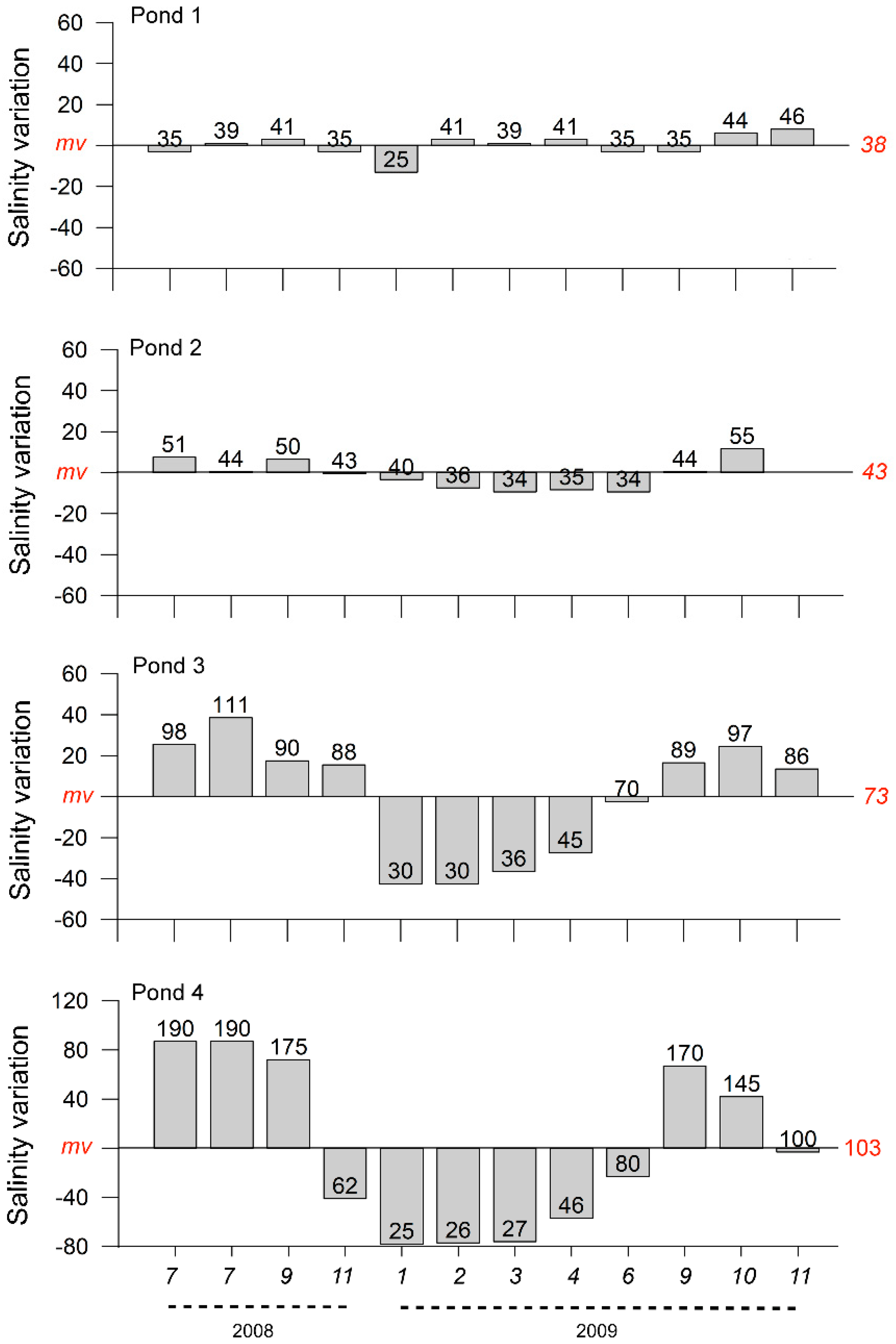
3.1. Salinity
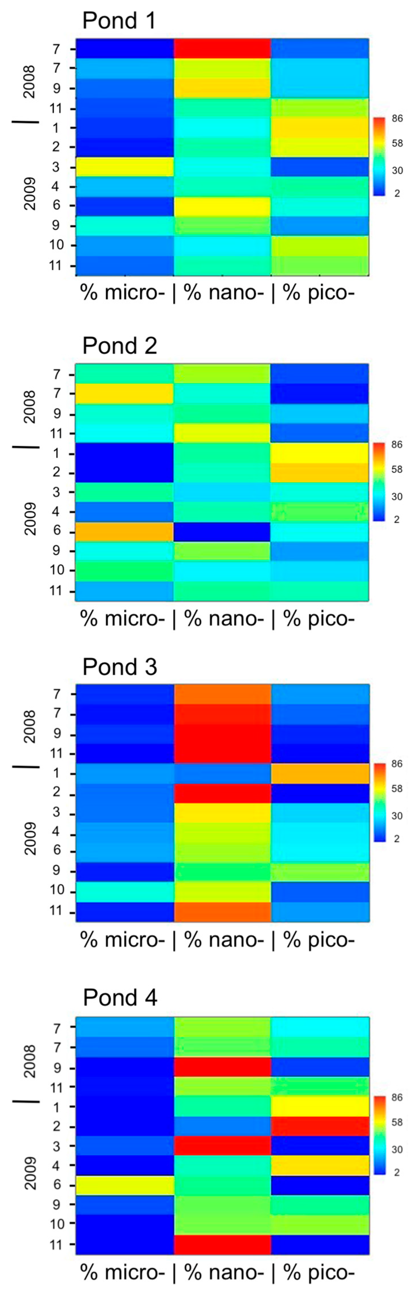
3.2. Total Phytoplankton Biomass and Size Classes
3.3. Chemotaxonomical Composition of Phytoplankton
3.4. Similarity Tests and Neighbor Joining Clustering Analyses
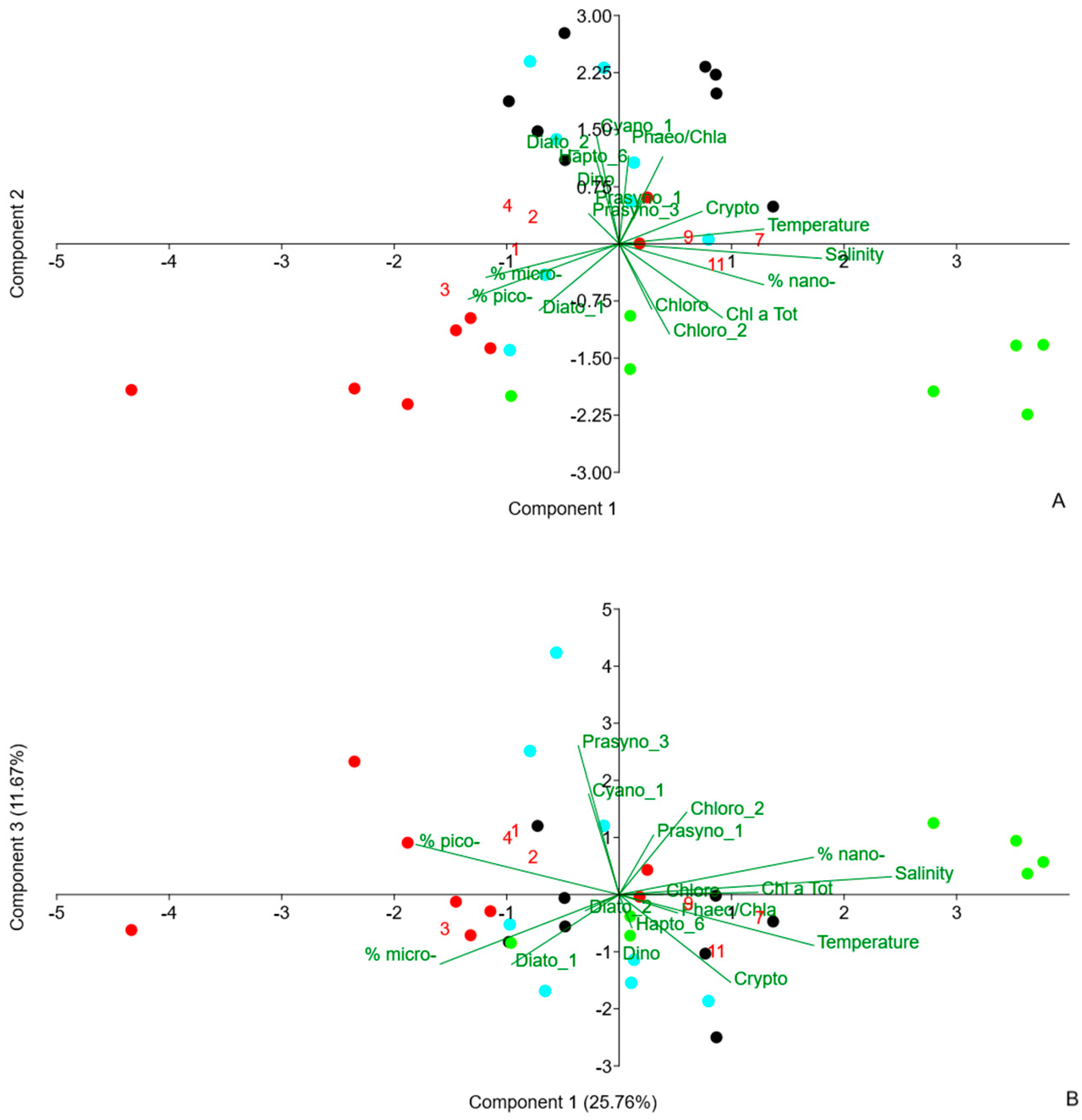
3.5. PCA
4. Discussion
5. Conclusions
Supplementary Materials
Author Contributions
Funding
Data Availability Statement
Acknowledgments
Conflicts of Interest
References
- Petanidou, T. Salt-Salt in European History and Civilization. In Hellenic Saltworks S.A.; Bilingual Publication: Athens, Greece, 1997. [Google Scholar]
- Petanidou, T. Non-typical salinas and salt harvesting in the Mediterranean. In Salt and Salinas in the Mediterranean; Neves, R., Petanidou, T., Rufino, R., Pinto, S., Eds.; Lisbon Municipality of Figueira da Foz-ALAS, Portugal, 2003; pp. 34–35. Available online: www.aegean.gr/alas/final_publ.htm (accessed on 4 October 2022).
- Britton, R.H.; Johnson, A.R. An ecological account of a Mediterranean salina: The Salin de Giraud, Camargue (S. France). Biol. Conserv. 1987, 42, 185–230. [Google Scholar] [CrossRef]
- Velasquez, C.R. Managing artificial saltpans as a waterbird habitat: Species’ responses to water level manipulation. Colonial Waterbirds 1992, 15, 43–55. [Google Scholar] [CrossRef]
- Masero, J.A. Assessing alternative anthropogenic habitats for conserving waterbirds: Salinas as buffer areas against the impact of natural habitat loss for shorebirds. Biodivers. Conserv. 2003, 12, 1157–1173. [Google Scholar] [CrossRef]
- Soares, R.H.R.D.H.; Assunção, C.A.D.; Fernandez, F.D.O.; Marinho-Soriano, E. Identification and analysis of ecosystem services associated with biodiversity of saltworks. Ocean Coast. Manag. 2018, 163, 278–284. [Google Scholar] [CrossRef]
- Pedrós-Alió, C.; Calderón-Paz, J.I.; MacLean, M.H.; Medina, G.; Marrasé, C.; Gasol, J.M.; Guixa-Boixereu, N. The microbial food web along salinity gradients. FEMS Microbiol. Ecol. 2000, 32, 143–155. [Google Scholar] [CrossRef]
- Oren, A. Diversity of halophilic microorganisms: Environments, phylogeny, physiology, and applications. J. Ind. Microbiol. Biotechnol. 2002, 28, 56–63. [Google Scholar] [CrossRef]
- Oren, A. Saltern evaporation ponds as model systems for the study of primary production processes under hypersaline conditions. Aquat. Microb. Ecol. 2009, 56, 193–204. [Google Scholar] [CrossRef]
- Reynolds, C.S. The Ecology of Phytoplankton; Cambridge University Press: Cambridge, UK, 2006. [Google Scholar] [CrossRef]
- Padisak, J.; Naselli-Flores, L. Phytoplankton in extreme environments: Importance and consequences of habitat permanency. Hydrobiologia 2021, 848, 157–176. [Google Scholar] [CrossRef]
- Bonifazi, A.; Galli, S.; Gravina, M.F.; Ventura, D. Macrozoobenthos Structure and Dynamics in a Mediterranean Hypersaline Ecosystem with Implications for Wetland Conservation. Water 2023, 15, 1411. [Google Scholar] [CrossRef]
- Teodoresco, E.C. Observations morphologiques et biologiques sur le genere Dunaliella. Rev. Générale De Bot. 1906, 18, 353–371, and 18, 409–427. [Google Scholar]
- Artom, C. Osservazioni Generali sull’Artemia Salina delle Saline di Cagliari; Zoologischer Anzeiger XXIX No. 9: Leiden, The Netherlands, 1905; pp. 284–291. [Google Scholar]
- Artom, C. L’origine e l’evoluzione della partenogenesi attraverso i differenti biotipi di una specie collettiva (Artemia salina L.) con speciale riferimento al biotipo diploide partenogenetico di Sète. Mem. d.r. Accad. D’Italia II 1931, 2, 219–273. [Google Scholar]
- Diaz, S.; Cabido, M. Vive la différence: Plant functional diversity matters to ecosystem processes. Trends in Ecology and Evolution. Trends Ecol. Evol. 2001, 16, 646–655. [Google Scholar] [CrossRef]
- Petchey, O.L.; Gaston, K.J. Functional diversity (FD), species richness, and community composition. Ecol. Lett. 2002, 5, 402–411. [Google Scholar] [CrossRef]
- Mason, N.W.H.; Mouillot, D.; Lee, W.G.; Wilson, J.B. Functional richness, functional evenness and functional divergence: The primary components of functional diversity. Oikos 2005, 111, 112–118. [Google Scholar] [CrossRef]
- Grime, J.P. Trait convergence and trait divergence in herbaceous plant communities: Mechanisms and consequences. J. Veg. Sci. 2006, 17, 255–260. [Google Scholar] [CrossRef]
- McGill, B.J.; Enquist, B.J.; Weiher, E.; Westoby, M. Rebuilding community ecology from functional traits. Trends Ecol. Evol. 2006, 21, 178–185. [Google Scholar] [CrossRef]
- Cloern, J.E.; Jassby, A.D. Patterns and Scales of Phytoplankton Variability in Estuarine–Coastal Ecosystems. Estuaries Coasts 2010, 33, 230–241. [Google Scholar] [CrossRef] [Green Version]
- Roscher, C.; Schumacher, J.; Gubsch, M.; Lipowsky, A.; Weigelt, A.; Buchmann, N.; Schmid, B.; Schulze, E.D. Using Plant Functional Traits to Explain Diversity–Productivity Relationships. PLoS ONE 2012, 7, e36760. [Google Scholar] [CrossRef]
- Roselli, L.; Litchman, E.; Stanca, E.; Cozzoli, F.; Basset, A. Individual trait variation in phytoplankton communities across multiple spatial scales. J. Plankton Res. 2017, 39, 577–588. [Google Scholar] [CrossRef] [Green Version]
- Ayadi, H.; Abid, O.; Elloumi, J.; Bouaïn, A.; Sime-Ngando, T. Structure of the phytoplankton communities in two lagoons of different salinity in the Sfax saltern (Tunisia). J. Plankton Res. 2004, 26, 669–679. [Google Scholar] [CrossRef] [Green Version]
- Bec, B.; Husseini-Ratrema, J.; Collos, Y.; Souchu, P.; Vaquer, A. Phytoplankton seasonal dynamics in a Mediterranean coastal lagoon: Emphasis on the picoeukaryote community. J. Plankton Res. 2005, 27, 881–894. [Google Scholar] [CrossRef] [Green Version]
- Evagelopoulos, A.; Spyrakos, E.; Koutsoubas, D. Phytoplankton and macrofauna in the low salinity ponds of a productive solar saltworks: Spatial variability of community structure and its major abiotic determinants. Glob. Nest J. 2009, 11, 64–72. [Google Scholar] [CrossRef] [Green Version]
- Elliott, M.; Whitfield, A.K. Challenging paradigms in estuarine ecology and management. Estuar. Coast. Shelf Sci. 2011, 94, 306–314. [Google Scholar] [CrossRef]
- Estrada, M.; Henriksen, P.; Gasol, J.M.; Casamayor, E.O.; Pedrós-Alió, C. Diversity of planktonic photoautotrophic microorganisms along a salinity gradient as depicted by microscopy, flow cytometry, pigment analysis and DNA-based methods. FEMS Microbiol. Ecol. 2004, 49, 281–293. [Google Scholar] [CrossRef]
- Asencio, A.D. Permanent salt evaporation ponds in a semi-arid Mediterranean region as model systems to study primary production processes under hypersaline conditions. Estuar. Coast. Shelf Sci. 2013, 6, 124. [Google Scholar] [CrossRef]
- Wilson, D.S. Complex Interactions in Metacommunities, with Implications for Biodiversity and Higher Levels of Selection. Ecology 1992, 73, 1984–2000. [Google Scholar] [CrossRef]
- Leibold, M.A.; Holyoak, M.; Mouquet, N.; Amarasekare, P.; Chase, J.M.; Hoopes, M.F.; Holt, R.D.; Shurin, J.B.; Law, R.; Tilman, D.; et al. The metacommunity concept: A framework for multi-scale community ecology. Ecol. Lett. 2004, 7, 601–613. [Google Scholar] [CrossRef]
- Declerck, S.A.; Winter, C.; Shurin, J.B.; Suttle, C.A.; Matthews, B. Effects of patch connectivity and heterogeneity on metacommunity structure of planktonic bacteria and viruses. ISME J. 2013, 7, 533–542. [Google Scholar] [CrossRef]
- Dallas, T.A.; Kramer, A.M.; Zokan, M.; Drake, J.M. Ordination obscures the influence of environment on plankton metacommunity structure. Limnol. Oceanogr. Lett. 2016, 1, 54–61. [Google Scholar] [CrossRef] [Green Version]
- Bortolini, J.C.; Pineda, A.; Rodrigues, L.C.; Jati, S.; Velho, L.F.M. Environmental and spatial processes influencing phytoplankton biomass along a reservoirs-river-floodplain lakes gradient: A metacommunity approach. Freshw. Biol. 2017, 62, 1756–1767. [Google Scholar] [CrossRef]
- Di Maio, A. Campo Idrodinamico Nella Salina di Tarquinia a Supporto di studi Ecologici e di Soluzioni Operative: Applicazione di un Modello Numerico ad Elementi Finiti. Ph.D. Thesis, Università degli Studi della Tuscia, Viterbo, Italy, 2006; pp. 1–129. [Google Scholar]
- Cimmaruta, R.; Blasi, S.; Angeletti, D.; Nascetti, G. The recent history of the Tarquinia Salterns offers the opportunity to investigate parallel changes at the habitat and biodiversity levels. Transit. Waters Bull. 2010, 4, 2. [Google Scholar] [CrossRef]
- Allavena, S.; Zapparoli, M. Gestione e tutela della Riserva Naturale di Popolamento Animale Salina di Tarquinia. In L’ambiente della Tuscia Laziale; Olmi, M., Zapparoli, M., Eds.; Union Printing: Viterbo, Italy, 1992; pp. 189–192. [Google Scholar]
- Allavena, S.; Zapparoli, M. Aspetti faunistici della Riserva Naturale di Popolamento Animale Salina di Tarquinia e aree adiacenti. In L’ambiente della Tuscia Laziale; Olmi, M., Zapparoli, M., Eds.; Union Printing: Viterbo, Italy, 1992; pp. 209–216. [Google Scholar]
- Serra, L.; Casini, L.; Della Toffola, M.; Magnani, A.; Meschini, A.; Tinarelli, R. Results of a survey on wader spring migration in Italy (March–May 1990). Wader Study Group Bull. 1992, 66, 54–60. [Google Scholar]
- Angeletti, D.; Cimmaruta, R.; Nascetti, G. Genetic diversity of the killifish Aphanius fasciatus paralleling the environmental changes of Tarquinia salterns habitat. Genetica 2010, 138, 1011–1021. [Google Scholar] [CrossRef]
- Bellisario, B.; Novelli, C.; Cerfolli, F.; Angeletti, D.; Cimmaruta, R.; Nascetti, G. The ecological restoration of the Tarquinia Salterns drives the temporal changes in the benthic community structure. Transit. Waters Bull. 2010, 4, 3–62. [Google Scholar]
- Bellisario, B.; Carere, C.; Cerfolli, F.; Angeletti, D.; Nascetti, G.; Cimmaruta, R. Infaunal macrobenthic community dynamics in a manipulated hyperhaline ecosystem: A long-term study. Aquat. Biosyst. 2013, 9, 20. [Google Scholar] [CrossRef] [Green Version]
- Mattiucci, S.; Sbaraglia, G.L.; Palomba, M.; Filippi, S.; Paoletti, M.; Cipriani, P.; Nascetti, G. Genetic identification and insights into the ecology of Contracaecum rudolphii A and C. rudolphii B (Nematoda: Anisakidae) from cormorants and fish of aquatic ecosystems of Central Italy. Parasitol. Res. 2020, 119, 1243–1257. [Google Scholar] [CrossRef]
- Jeffrey, S.W.; Humphrey, G.F. New spectrophotometric equations for determining chlorophylls a, b, c1 and c2 in higher plants, algae and natural phytoplankton. Biochem. Physiol. Der Pflanz. 1975, 167, 191–194. [Google Scholar] [CrossRef]
- Vidussi, F.; Claustre, H.; Bustillos-Guzman, J.; Cailliau, C.; Marty, J.C. Determination of chlorophylls and carotenoids of marine phytoplankton: Separation of chlorophyll a from divinyl-chlorophyll a and zeaxanthin from lutein. J. Plankton Res. 1996, 18, 2377–2382. [Google Scholar] [CrossRef] [Green Version]
- Mantoura, R.F.C.; Repeta, D.J. Calibration methods for HPLC. In Phytoplankton Pigments in Oceanography; Jeffrey, W., Mantoura, R.F.C., Wright, S.W., Eds.; UNESCO Publishing: Paris, France, 1997; pp. 407–428. [Google Scholar]
- Latasa, M. Improving estimations of phytoplankton class abundances using CHEMTAX. Mar. Ecol. Prog. Ser. 2007, 329, 13–21. [Google Scholar] [CrossRef] [Green Version]
- Saitou, N.; Nei, M. The neighbor-joining method: A new method for reconstructing phylogenetic trees. Mol. Biol. Evol. 1987, 4, 406–425. [Google Scholar] [CrossRef]
- Clarke, K.R. Non-parametric multivariate analysis of changes in community structure. Aust. J. Ecol. 1993, 18, 117–143. [Google Scholar] [CrossRef]
- Nascetti, G.; Scardi, M.; Fresi, E.; Cimmaruta, R.; Bondanelli, P.; Gatti, S.; Blasi, S.; Serrano, S.; Meschini, L.; Lanera, P.; et al. Caratterizzazione ecologica delle Saline di Tarquinia al fine di un loro recupero e per lo sviluppo dell’acquacoltura. Biol. Mar. Med. 1998, 5, 1365–1374. [Google Scholar]
- Davis, J.S. Structure, function and management of the biological system for seasonal solar saltworks. Glob. Nest J. 2000, 2, 217–226. [Google Scholar]
- Walmsley, J.G. The ecological importance of Mediterranean Salinas. In Saltworks: Preserving Saline Coastal Ecosystems; Korovessis, N., Lekkas, T.D., Eds.; Glob Nest-Hellenic Saltworks S.A.: Athens, Greece, 2000; pp. 81–95. [Google Scholar]
- Crisman, T.; Takavakoglou, V.; Alexandridis, T.; Antonopoulos, V.; Zalidis, G. Rehabilitation of Abandoned Saltworks to Maximize Conservation, Ecotourism and Water Treatment Potential. Glob. Nest J. 2009, 11, 24–31. [Google Scholar]
- Salmaso, N.; Naselli-Flores, L.; Padisák, J. Functional classifications and their application in phytoplankton ecology. Freshw. Biol. 2015, 60, 603–619. [Google Scholar] [CrossRef] [Green Version]
- Weithoff, G.; Beisner, B.E. Measures and Approaches in Trait-Based Phytoplankton Community Ecology—From Freshwater to Marine Ecosystems. Front. Mar. Sci. 2019, 6, 40. [Google Scholar] [CrossRef] [Green Version]
- Kim, H.G.; Hong, S.; Kim, D.K.; Joo, G.J. Drivers shaping episodic and gradual changes in phytoplankton community succession. Taxonomic versus functional groups. Sci. Total Environ. 2020, 734, 138940. [Google Scholar] [CrossRef]
- Kruk, C.; Mazzeo, N.; Lacerot, G.; Reynolds, C.S. Classification schemes for phytoplankton: A local validation of a functional approach to the analysis of species temporal replacement. J. Plankton Res. 2002, 24, 901–912. [Google Scholar] [CrossRef]
- Wentzky, V.C.; Tittel, J.; Jäger, C.G.; Bruggeman, J.; Rinke, K. Seasonal succession of functional traits in phytoplankton communities and their interaction with trophic state. J. Ecol. 2020, 108, 1649–1663. [Google Scholar] [CrossRef] [Green Version]
- Abid, O.; Sellami-Kammoun, A.; Ayadi, H.; Drira, Z.; Bouain, A.; Aleya, L. Biochemical adaptation of phytoplankton to salinity and nutrient gradients in a coastal solar saltern, Tunisia. Estuar. Coast. Shelf Sci. 2008, 80, 391–400. [Google Scholar] [CrossRef]
- Madkour, F.F.; Gaballah, M.M. Phytoplankton assemblage of a solar saltern in Port Fouad, Egypt. Oceanologia 2012, 54, 687–700. [Google Scholar] [CrossRef]
- Costa, R.S.; Molozzi, J.; Hepp, L.U.; Rocha, R.M.; Barbosa, J.E.L. Diversity partitioning of a phytoplankton community in semiarid salterns. Mar. Freshw. Res. 2016, 67, 238–245. [Google Scholar] [CrossRef]
- Tempesta, S.; Paoletti, M.; Pasqualetti, M. Morphological and molecular identification of a strain of the unicellular green alga Dunaliella sp. isolated from Tarquinia salterns. Transit. Waters Bull. 2010, 4, 60–70. [Google Scholar]
- Pasqualetti, M.; Tempesta, S. Dunaliella salina: Isolamento, determinazione e caratterizzazione di popolazioni identificate nelle vasche delle Saline di Tarquinia. In 2014–La Riserva Naturale Statale “Saline di Tarquinia”; Colletti, L., Ed.; Corpo forestale dello Stato, Ufficio territoriale per la Biodiversità di Roma: Rome, Italy, 2014; pp. 65–73. [Google Scholar]
- Pasqualetti, M.; Bernini, R.; Carletti, L.; Crisante, F.; Tempesta, S. Salinity and nitrate concentration on the growth and carotenoids accumulation in a strain of Dunaliella salina (Chlorophyta) cultivated under laboratory conditions. Transit. Waters Bull. 2010, 4, 94–104. [Google Scholar]
- Stauffer, D.; Aharony, A. Introduction to Percolation Theory, 2nd ed.; Taylor and Francis: Abingdon, UK, 1992. [Google Scholar] [CrossRef]
- Presley, S.; Higgins, C.; Willig, M. A comprehensive framework for the evaluation of metacommunity structure. Oikos 2010, 119, 908–917. [Google Scholar] [CrossRef]
- Sadoul, N.; Walmsley, J.; Charpentier, B. Salinas and Nature Conservation. In Conservation of Mediterranean Wetlands; Crivelli, A.J., Jalbert, J., Eds.; 9. MedWet/Tour du Valat Publications: Arles, France, 1998. [Google Scholar]
- Gálvez, Á.; Peres-Neto, P.R.; Castillo-Escrivà, A.; Bonilla, F.; Camacho, A.; García-Roger, E.M.; Iepure, S.; Miralles-Lorenzo, J.; Monrós, J.S.; Olmo, C.; et al. Inconsistent Response of Taxonomic Groups to Space and Environment in Mediterranean and Tropical Pond Metacommunities. Ecology 2023, 104, e3835. [Google Scholar] [CrossRef]
- Amat, F.; Hontoria, F.; Navarro, J.C.; Vieira, N.; Mura, G. Biodiversity loss in the genus Artemia in the Western Mediterranean Region. Limnetica 2007, 26, 177–194. [Google Scholar] [CrossRef]


| Lat. N | Lon. E | Depth (cm) | |
|---|---|---|---|
| Pond 1 | 42.210502 | 11.70997 | 100 |
| Pond 2 | 42.205383 | 11.71502 | 80 |
| Pond 3 | 42.199698 | 11.72096 | ~30 |
| Pond 4 | 42.195687 | 11.72161 | ~15 |
| Anosim Test—Functional Groups | p-Values. Uncorrected Significance | ||||||
|---|---|---|---|---|---|---|---|
| Permutation N: | 9999 | Pond 1 | Pond 2 | Pond 3 | Pond 4 | ||
| Mean rank within: | 158.9 | Pond 1 | 0.4272 | 0.0017 | 0.0004 | ||
| Mean rank between: | 235.2 | Pond 2 | 0.4272 | 0.0055 | 0.0009 | ||
| R: | 0.3507 | Pond 3 | 0.0017 | 0.0055 | 0.4403 | ||
| p (same): | 0.0001 | Pond 4 | 0.0004 | 0.0009 | 0.4403 | ||
| Simper Test—Functional groups | |||||||
| Taxon | Av. Dissim | Contrib. % | Cumul. % | Pond 1 | Pond 2 | Pond 3 | Pond 4 |
| Chloro2 | 19.79 | 29 | 29 | 5.91 | 6.1 | 49.5 | 58 |
| Diato1 | 14.69 | 21.53 | 50.53 | 18 | 30.1 | 36.4 | 31.5 |
| Diato2 | 9 | 13.24 | 63.77 | 27.8 | 10.6 | 0.973 | 3.53 |
| Dino | 8.34 | 12.22 | 75.99 | 14.4 | 24.1 | 0.281 | 0.0814 |
| Cyano_1 | 7 | 10.15 | 86.14 | 16.3 | 17.3 | 0.367 | 0.98 |
| Crypto | 6 | 9 | 94.82 | 14.8 | 5.22 | 8.34 | 2.68 |
| Prasyno1 | 1 | 2 | 96.7 | 1.73 | 2.48 | 1.17 | 1.11 |
| Chloro | 1 | 2 | 98.47 | 0.0613 | 1.79 | 2.66 | 1.21 |
| Prasyno3 | 0.8032 | 1 | 99.64 | 0.121 | 2.18 | 0.303 | 0.957 |
| Hapto6 | 0.2436 | 0.357 | 100 | 0.859 | 0.104 | 0.0243 | 0.0214 |
| Anosim Test—Size classes | p-values. Uncorrected significance | ||||||
| Permutation N: | 9999 | Pond 1 | Pond 2 | Pond 3 | Pond 4 | ||
| Mean rank within: | 513.1 | Pond 1 | 0.1742 | 0.0283 | 0.3073 | ||
| Mean rank between: | 580.2 | Pond 2 | 0.1742 | 0.0002 | 0.0161 | ||
| R: | 0.119 | Pond 3 | 0.0283 | 0.0002 | 0.1401 | ||
| p (same): | 0.0051 | Pond 4 | 0.3073 | 0.0161 | 0.1401 | ||
| Simper Test–Size classes | |||||||
| Taxon | Av. Dissim | Contrib. % | Cumul. % | Pond 1 | Pond 2 | Pond 3 | Pond 4 |
| % nano- | 12.35 | 36.28 | 36.28 | 46 | 37.2 | 64.7 | 53.9 |
| % pico- | 11.98 | 35.21 | 71.49 | 36.2 | 30.6 | 22.6 | 35.5 |
| % micro- | 10 | 28.51 | 100 | 17.8 | 32.2 | 12.7 | 10.5 |
| Anosim Test—Functional Groups | p-Values. Uncorrected Significance | |||||||||||
|---|---|---|---|---|---|---|---|---|---|---|---|---|
| Permutation N: | 9999 | July | Sept. | Nov. | Jan. | Feb. | Mar. | April | ||||
| Mean rank within: | 211.8 | July | 0.4221 | 0.7028 | 0.6576 | 0.3562 | 0.7466 | 0.7646 | ||||
| Mean rank between: | 202.3 | Sept. | 0.4221 | 0.4054 | 0.1731 | 0.46 | 0.4007 | 0.3377 | ||||
| R: | −0.0466 | Nov. | 0.7028 | 0.4054 | 0.2559 | 0.1997 | 0.3736 | 0.5565 | ||||
| p (same): | 0.6919 | Jan. | 0.6576 | 0.1731 | 0.2559 | 0.5484 | 0.4283 | 0.5446 | ||||
| Fabr. | 0.3562 | 0.46 | 0.1997 | 0.5484 | 0.9705 | 1 | ||||||
| Mar. | 0.7466 | 0.4007 | 0.3736 | 0.4283 | 0.9705 | 0.7257 | ||||||
| April | 0.7646 | 0.3377 | 0.5565 | 0.5446 | 1 | 0.7257 | ||||||
| SIMPER TEST—Functional groups | ||||||||||||
| Taxon | Av. dissim | Contrib. % | Cumul. % | July | Sept. | Nov. | Jan. | Feb. | Mar. | April | ||
| Chloro2 | 17.49 | 26.95 | 26.95 | 34.3 | 43.6 | 27.8 | 32.6 | 10 | 20.3 | 23.7 | ||
| Diato1 | 14.66 | 22.59 | 49.54 | 30 | 5.71 | 21.3 | 37.1 | 40.4 | 38.4 | 26.1 | ||
| Diato2 | 9 | 13.68 | 63.22 | 4.2 | 22.7 | 1.28 | 3.88 | 26.9 | 13.2 | 12.6 | ||
| Dino | 8 | 11.95 | 75.17 | 8.88 | 8.15 | 22.5 | 1.42 | 6.11 | 13.8 | 13.7 | ||
| Cyano_1 | 6 | 10.01 | 85.17 | 7.85 | 4.8 | 0.192 | 20.6 | 12 | 6.9 | 15 | ||
| Crypto | 6 | 9 | 94.56 | 11.1 | 11.3 | 24.5 | 0.427 | 0 | 3.54 | 0.217 | ||
| Prasyno1 | 1.35 | 2 | 96.64 | 1.44 | 2.67 | 0.47 | 0.733 | 0.645 | 0.075 | 7.03 | ||
| Chloro | 1 | 2 | 98.41 | 1.48 | 0.865 | 1.47 | 0 | 1.41 | 3.87 | 0.35 | ||
| Prasyno3 | 0.8088 | 1 | 99.65 | 0.474 | 0.208 | 0 | 2.71 | 2.11 | 0.005 | 1.27 | ||
| Hapto6 | 0.225 | 0.3467 | 100 | 0.287 | 0.055 | 0.515 | 0.42 | 0.47 | 0 | 0.0567 | ||
| Anosim Test—Size classes | p-values. uncorrected significance | |||||||||||
| Permutation N: | 9999 | July | Sept. | Nov. | Jan. | Feb. | Mar. | April | June | Oct. | ||
| Mean rank within: | 518.7 | July | 0.9241 | 0.4553 | 0.0165 | 0.0235 | 0.4402 | 0.1514 | 0.2835 | 0.1347 | ||
| Mean rank between: | 570 | Sept. | 0.9241 | 0.5909 | 0.0417 | 0.0351 | 0.3908 | 0.2693 | 0.2103 | 0.165 | ||
| R: | 0.09093 | Nov. | 0.4553 | 0.5909 | 0.1803 | 0.2247 | 0.2898 | 0.5754 | 0.2139 | 0.3316 | ||
| p (same): | 0.0621 | Jan. | 0.0165 | 0.0417 | 0.1803 | 0.6617 | 0.0624 | 0.4831 | 0.0734 | 0.827 | ||
| Feb. | 0.0235 | 0.0351 | 0.2247 | 0.6617 | 0.2248 | 0.2259 | 0.1178 | 0.5948 | ||||
| Mar. | 0.4402 | 0.3908 | 0.2898 | 0.0624 | 0.2248 | 0.0851 | 1 | 0.4567 | ||||
| Apr. | 0.1514 | 0.2693 | 0.5754 | 0.4831 | 0.2259 | 0.0851 | 0.2524 | 0.5281 | ||||
| June | 0.2835 | 0.2103 | 0.2139 | 0.0734 | 0.1178 | 1 | 0.2524 | 0.6075 | ||||
| Oct | 0.1347 | 0.165 | 0.3316 | 0.827 | 0.5948 | 0.4567 | 0.5281 | 0.6075 | ||||
| Simper Test–Size classes | ||||||||||||
| Taxon | Av. diss. | Con. % | Cum. % | July | Sept. | Nov. | Jan. | Feb. | Mar. | April | June | Oct. |
| % pico- | 12.21 | 36.4 | 36.4 | 19.2 | 24 | 27.6 | 51.1 | 50.6 | 18.4 | 44 | 23.9 | 42.9 |
| % nano- | 11.97 | 35.67 | 72.07 | 59.8 | 58.3 | 61.2 | 36.1 | 44.2 | 50.8 | 41.5 | 38.6 | 35.5 |
| % micro- | 9.37 | 27.93 | 100 | 21 | 17.6 | 11.1 | 12.9 | 5.17 | 30.8 | 14.5 | 37.5 | 21.6 |
Disclaimer/Publisher’s Note: The statements, opinions and data contained in all publications are solely those of the individual author(s) and contributor(s) and not of MDPI and/or the editor(s). MDPI and/or the editor(s) disclaim responsibility for any injury to people or property resulting from any ideas, methods, instructions or products referred to in the content. |
© 2023 by the authors. Licensee MDPI, Basel, Switzerland. This article is an open access article distributed under the terms and conditions of the Creative Commons Attribution (CC BY) license (https://creativecommons.org/licenses/by/4.0/).
Share and Cite
Bolinesi, F.; Talamo, A.; Mangoni, O. Temporal Evolution of Phytoplankton Metacommunity in a Disused Mediterranean Saltwork. Water 2023, 15, 2419. https://doi.org/10.3390/w15132419
Bolinesi F, Talamo A, Mangoni O. Temporal Evolution of Phytoplankton Metacommunity in a Disused Mediterranean Saltwork. Water. 2023; 15(13):2419. https://doi.org/10.3390/w15132419
Chicago/Turabian StyleBolinesi, Francesco, Annunziata Talamo, and Olga Mangoni. 2023. "Temporal Evolution of Phytoplankton Metacommunity in a Disused Mediterranean Saltwork" Water 15, no. 13: 2419. https://doi.org/10.3390/w15132419