Evolution Pattern of Blue–Green Space in New Urban Districts and Its Driving Factors: A Case Study of Zhengdong New District in China

Abstract

Understanding the spatial–temporal evolution of the blue–green space (BGS) is crucial for urban planning and ecological security protection. However, the evolutionary patterns and driving factors of the BGS in new urban districts remain unclear. Based on the classical qualitative models, “patch–corridor–matrix” and “sustainability prism”, this study adopted the land use transition matrix and landscape index to quantify evolution patterns, and Pearson correlation and geographical detector analysis methods to reveal the driving factors. Taking Zhengdong New District as a case study, the results indicated the following: (1) The BGS rate was reduced by 35% from 2003 to 2021, with the most significant decrease in cultivated lands. (2) The evolution pattern of BGS alternated sequentially among ecological, disorderly, and balanced states. Among them, urban green spaces tended towards a more stable and aggregated state. Other BGSs became more fragmented and discontinuous. (3) The “sustainability prism” model consists of four driving factors, including social economy, rainwater safety, ecological liveability, and physical geography. (4) Socioeconomic factors significantly decreased the BGS, as indicated by the correlation coefficients of −0.988 and −0.978 between built-up areas and population and gross domestic products, respectively. Physical geographic factors played weak roles in the evolution of the BGS. Meanwhile, rainwater safety and ecological liveability positively affected the BGS.

1. Introduction

Rapid urbanisation makes new urban districts increasingly crucial for supporting economic development and urban construction. However, urbanisation reduces blue–green space (BGS), such as rivers, dikes, and paddy fields, as they are occupied by urban land [1,2]. Inappropriate development and unreasonable planning of BGS are common problems in new urban districts [3]. Accurately assessing the evolution process of BGS is crucial for addressing these problems. Therefore, this study attempts to clarify the spatial–temporal evolution and driving factors of the BGS in new urban districts, conforming to “ecological security bottom line protection” during the planning transformation.

BGS generally refers to an open spatial system composed of all kinds of blue and green spaces in a city [4,5]. Green spaces include agricultural and ecological spaces, such as farmlands, forests, grasslands, parks, and protective green belts in urban areas, and blue spaces are the water bodies of various forms, such as rivers, lakes, reservoirs, ponds, beaches, and swamps [5,6]. These open spaces play a crucial role in regulating climate [7], preserving biodiversity [8], promoting human health [9], and improving the quality of life [10,11]. However, China’s ecological space area has shown a downward trend for nearly two decades [12]. The BGS is essential for implementing an ecological priority strategy in territorial spatial planning. The planning and design strategy for BGS suggests the rational construction of ecological patterns. And it is an essential basis for land use decisions [13] and sustainable urban development [14].

Regarding evolutionary patterns, current research has primarily agreed with the conclusion that urban expansion is the leading cause of the decline in BGS. This process is most prominent in Asian, Australian, and global cities represented by the UK [12,15,16]. Most scholars use the landscape pattern index to analyse the spatial distribution characteristics of BGS [17,18,19], enabling the quantification of the dynamic patterns of BGS. For example, landscape pattern indices of land use change in different regions of Nevada, the central United States, and the southern United States were easily quantified, described, and compared using the Frastates software [20]. Also, urban built-up areas in Wuhan occupied the blue–green space intensively and decreased heterogeneity, resulting in increased landscape fragmentation and reduced heterogeneity [21]. Other scholars have focused on the evolutionary patterns and mechanisms of specific types of BGS, such as urban green spaces [22]. But few studies have systematically described the landscape’s structure, function, and dynamics, potentially resulting in inaccurate urban planning.

Regarding evolutionary mechanisms, many scholars agree that socioeconomic and physical geographical factors influence the evolution of BGS and show different patterns of change [23,24]. They often use correlation analysis methods, such as multivariate logistic regression or geographical detectors, to establish a correlation between BGS and these factors [24,25]. However, these quantitative methods are mainly applied to the macro scale, such as in city areas or river basins. In practice, land use is also influenced by local policies and strategic land planning factors [26]. For example, some scholars have concluded that implementing the ecological protection red line policy has significantly altered the runoff and storage capacity of the surface [27]. In addition, all municipalities in France are required to implement blue and green infrastructure networks [28]. The BGS plays a role in rainwater storage. However, a unified research paradigm for driving mechanisms has yet to be established at the scale of new urban areas dominated by planning interventions.

In summary, spatial patterns and the driving mechanisms of BGS present unresolved problems. First, limited studies have analysed the evolution of BGS in new urban districts. Second, there is a lack of descriptive spatial language to describe pattern changes. Third, understanding the drivers of BGS spatial evolution is currently limited to the macro scale. Thus, this study proposes utilising the “patch–corridor–matrix” model [29] of landscape ecology and the “sustainability prism” [30] for planning and implementation. Referring to previous studies and research scales, this study defines cultivated land, woodland, grassland, wetland, urban green space, and water as components of BGS. The study area, Zhengdong New District, serves as a representative example of China’s new districts.

2. Theoretical Framework and Methods

2.1. Theoretical Framework

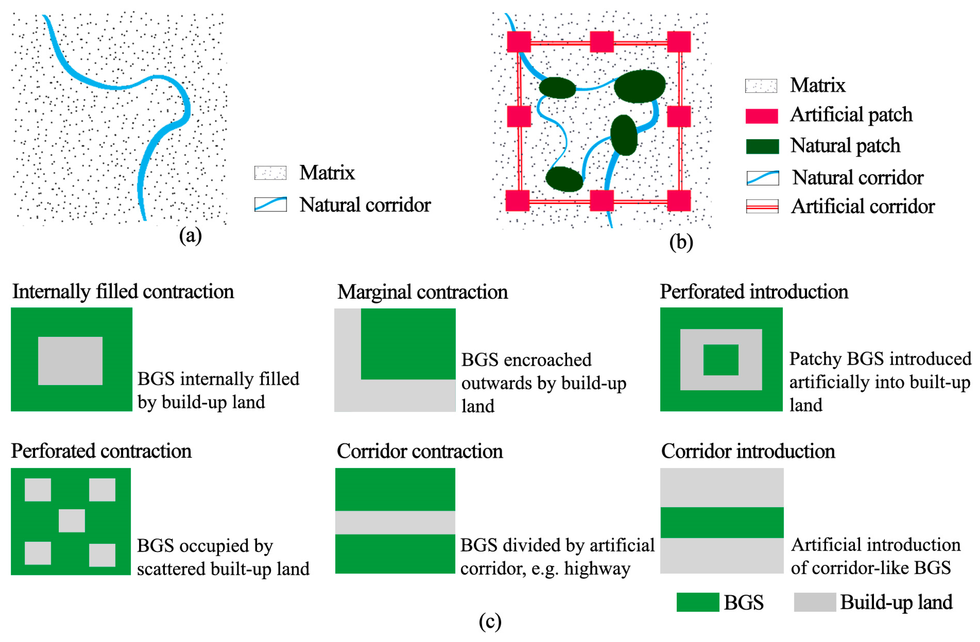
2.1.1. Theory of Spatial Pattern: “Patch–Corridor–Matrix” Model

Landscape ecology identifies natural or anthropogenic disturbances as the primary causes of spatial patterns across different scales. Before urbanisation, the BGS was primarily a continuous background structure. Later, the expansion of construction land led to the reduction, division, perforation, disappearance, and fragmentation of the BGS, forming space patches of different scales. Forman, an ecologist, proposed the “patch-corridor-matrix” model [31]. The matrix is the most extensive space, mainly in large agricultural ponds. Patches and corridors are embedded in the matrix [29,31]. On the one hand, a patch refers to a spatial unit that differs from the surrounding environment and displays a certain internal homogeneity. Patches serve as BGS that accommodate and eliminate rainwater, such as wetlands, woodlands, urban green spaces, and rural settlements. On the other hand, corridors are linear or band-like structures that differ from the adjacent environment and mainly consist of BGSs along rivers and their banks. Some scholars applied this model to construct ecological conservation networks [32] and rainwater safety patterns [33]. Therefore, it is evident that this model is appropriate for describing the spatial pattern of the BGS. In conclusion, the “patch–corridor–matrix” model provides a “spatial language” to describe the spatial dynamics of BGS and facilitate time-based comparisons. Based on existing studies, the evolution of the BGS is summarised as marginal contraction, internally filled contraction, perforated contraction, perforated introduction, and corridor cutting, which are determined by the interactions between the patch, corridor, and matrix (Figure 1).

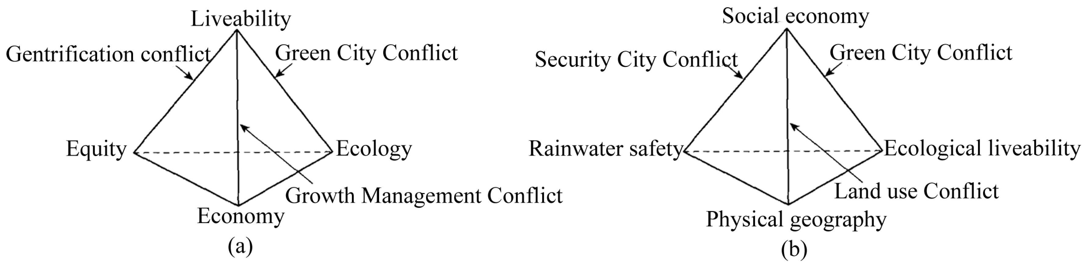
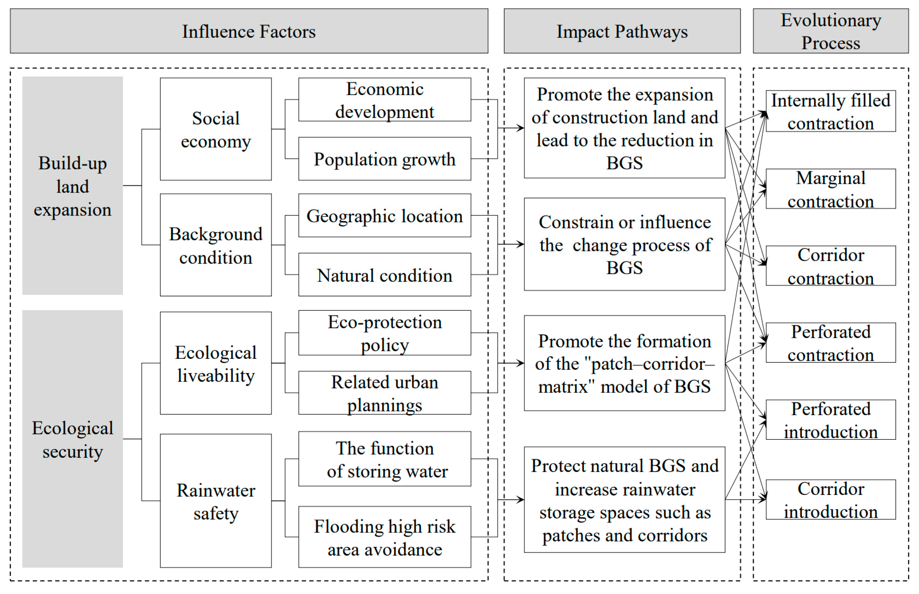
2.1.2. Theory of Driving Mechanism: “Sustainability Prism” Model

The “Sustainability prism” model was first applied to Denver regional planning and clearly showed the above goals’ interaction [34]. Urban planners use the “sustainability prism” model to understand the direct conflicts between stakeholders when developing and implementing plans [30]. The vertices of the prism initially represented the four goals of economy, equity, liveability, and ecology, with the central point representing the ideal or unattainable state. For the past 20 years, land use in Zhengdong New District has adhered to a specific plan, making it appropriate to utilise the sustainability prism model to explicate the spatial evolution mechanism of BGS.

As mentioned in the literature review [25,26], it is evident that the region’s physical geography and socioeconomic factors mainly influence blue–green space. In addition to socioeconomic factors, existing studies have established correlations between stormwater safety and ecological conservation with BGS [9,33]. Thus, the evolution of BGS should be determined by multiple factors, including social economy, physical geography, rainwater safety, and ecological liveability. These four factors are designated as the four vertices of the “Sustainability Prism” model (Figure 2), which is analysed quantitatively and qualitatively. This model demonstrates higher scientific validity than the commonly applied quantitative correlation analyses of several factors, such as social, economic, and natural factors with land use.

2.2. Methods

2.2.1. Land Use Transition Matrix

The land use transition matrix applies the Markov model to understand land use changes. It can quantify the structural characteristics, transfer direction, and degree of land types in different periods by listing their interconversion relationships in a matrix [35]. A comprehensive dynamic degree of land change can be derived based on the transfer matrix. And it refers to the degree of change of the whole land use type in a specific time range, which is an indicator for judging transformation hotspot areas [36]. The land use transition matrix and comprehensive dynamic degree of land change can be used to analyse the variation in BGS in Zhengdong New District regarding the number. It requires land use data for different periods. The general form of the transition matrix (Pij) and comprehensive dynamic degree of land change (S) are as follows:

$$P_{ij}=\left[\begin{array}{cccc}{P}_{11}& P_{12}& ...& P_{1n}\\ P_{21}& P_{22}& ...& P_{2n}\\ ...& ...& ...& ...\\ P_{n1}& P_{n2}& P_{n3}& P_{nn}\end{array}\right]$$

(1)

$$S=\left(\sum _{n=1}^m\frac{\Delta S_{i-j}}{S_i}\right)\times \frac{1}{T}\times 100\%$$

(2)

where P is the land area, i is the land use type at the beginning, j is the land use type at the end, n is the number of land use types, Si is the total area of land type i at the beginning of the study, ΔSi − j is the total area of land type i converted into land type j during the study period, and T is the year.

2.2.2. Landscape Index Analysis

Landscape index analysis was introduced to evaluate changes in the spatial clustering and connectivity characteristics of the BGS. The indices used in this study included the connectivity index (Connect), patch density index (PD), and aggregation index (AI), which are closely related to the “patch-corridor-matrix” model. All indices were quantified using Fragstats 4.2 software. These indices can be used to analyse the variation of BGS in Zhengdong New District regarding the spatial pattern. Connect refers to the connectivity between patches of the BGS based on the action distance. A higher Connect indicates higher connectivity. A higher PD indicates a higher degree of landscape fragmentation. AI indicates the degree of patch aggregation, reflecting the mutual dispersion of a certain number of elements. A higher AI indicates more significant aggregation, whereas a lower AI indicates greater dispersion [37]. The respective formulas are as follows:

$$Connect=\left(\sum _{j=k}^n{C}_{ijk}\right)/\left[\frac{n_i\left(n_i-1\right)}{2}\right]\times 100$$

(3)

$$PD=\left(n/A\right)\times \mathrm{10,000}\times 100$$

(4)

$$AI=\left[\sum _{i=1}^m\left(\frac{g_{ii}}{\mathit{max}{g}_{ii}}\right)p_i\right]\times 100$$

(5)

where $C_{ijk}$ is the connection between a given connection distance and the same type of patches within j and k (1 means connected, 0 means not connected), $n_i$ is the number of patches of landscape type i, $n$ is the number of patches, A is the area of the whole landscape or a landscape type, and $g_{ii}$ is the number of nodes between the image elements of patch type i.

2.2.3. Pearson Correlation Analysis

This study uses Pearson correlation analysis to measure the linear relationship between two normal continuous variables. This method is used to analyse the direct correlation between socioeconomic and BGS changes. The correlation coefficient r, measured between [−1, 1], reflects the degree of correlation between variables, identifying variables with 0.8 ≦ r ≦ 1 as strong positive correlation, variables with 0.3 ≦ r < 0.8 as weak positive correlation, variables with −0.3 ≦ r < 0.3 as no correlation, variables with −0.8 ≦ r < −0.3 as weak negative correlation, and variables with −1 ≦ r < −0.8 as strong negative correlation [38]. The calculation formula is as follows:

$$r=\frac{{\sum }_{i=1}^n(x_i-\overline{X}\left)\right(Y_i-\overline{Y})}{\sqrt{{\sum }_{i=1}^n(x_i-\overline{x{)}^2}}\sqrt{{\sum }_{i=1}^n(Y_i-\overline{Y{)}^2}}}$$

(6)

where $x_i$ and $Y_i$ represent the two variables; $\stackrel{-}{X}$ and $\stackrel{-}{Y}$ represent the mean of X and Y variables, respectively; n represents the number of samples.

2.2.4. Geographical Detector Analysis

A geographical detector is a set of statistical methods for detecting spatial heterogeneity and the magnitude of the explanatory power of the driving factors [39]. This study uses factor detection to identify the physical geography factors on the spatial variation in BGS and express the magnitude of the explanatory power of each driver on BGS variation by the q-value. Q-values range from 0 to 1, identifying factors with q > 0.5 as strong influence factors, factors with 0.4 < q < 0.5 as general influence factors, and factors with q < 0.4 as relatively weak influence factors [40], the model of which is as follows:

$$q=1-\frac{1}{N{\sigma }^2}\sum _{i=1}^n{N}_i{\sigma }_i^2$$

(7)

where $N_i$ and $N$ represent the number of the i-th layer region and the whole region, respectively; $n$ is the number of regions; $N_i{\sigma }_i^2$ and $N{\sigma }^2$ denote the variance in the i-th layer and whole region in the BGS, respectively.

3. Study Area and Materials

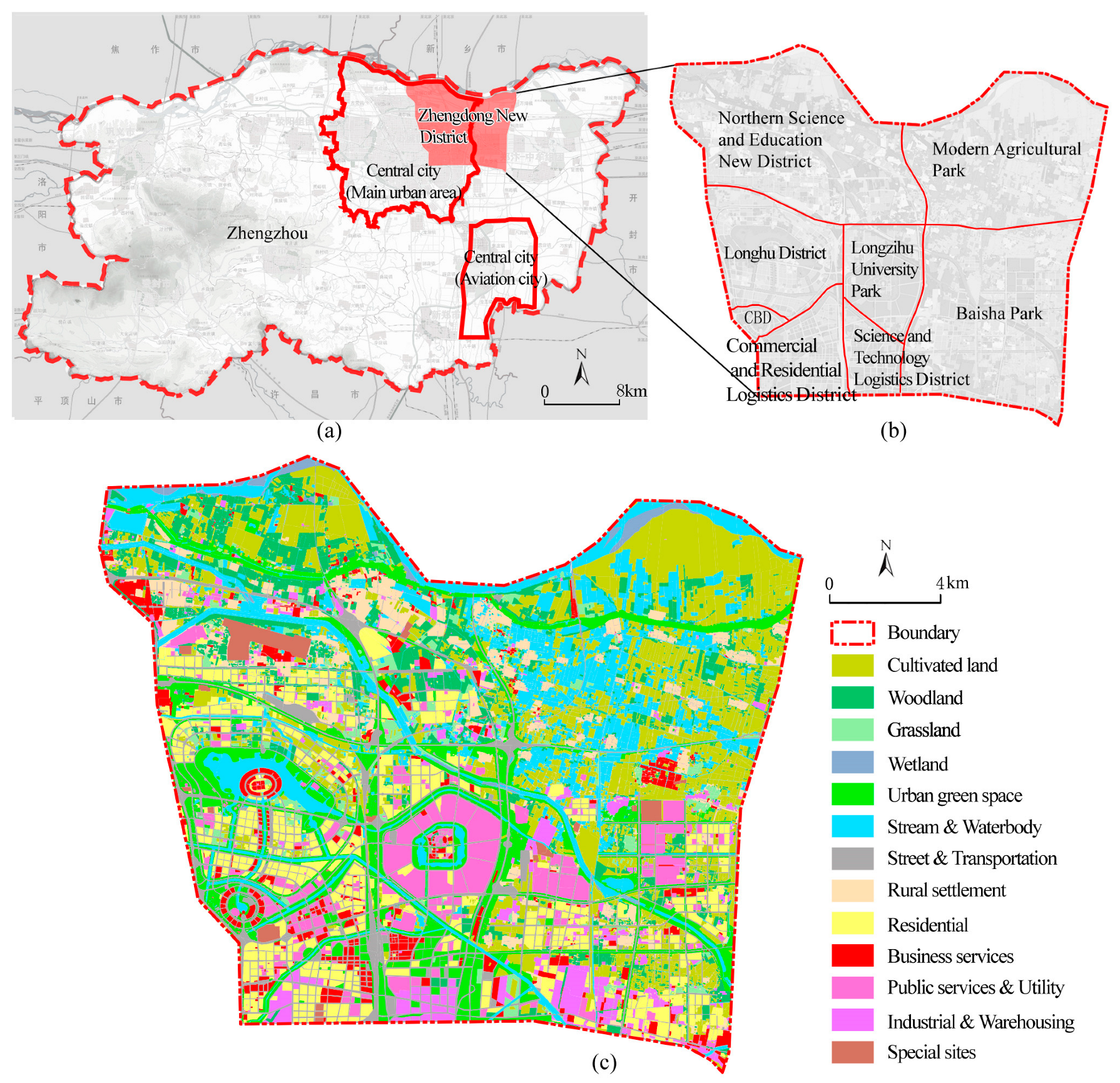
3.1. Study Area

Zhengdong New District is a typical example of urban space expansion driven by rapid urbanisation, which was launched in 2003. The district is situated in a low-lying region compared to the old city, experiencing year-round waterlogging with expansive swamplands and fish ponds before construction. The BGS has changed dramatically during the development process of the last two decades due to the new district occupying cultivated land, ponds, and ditches on a large scale while constructing several artificial lakes. In addition, the “7–20” heavy floods in 2021 severely impacted Zhengzhou. However, there is a gap in the research on the spatial evolution of BGS, which may lead to an inadequate scientific basis for constructing ecological safety networks. Therefore, Zhengdong New District serves as a representative case for this study.

The district extends from Zhongzhou Avenue to the west and is adjacent to the old city. It stretches as far as the Yellow River in the north, the Wansan Highway in the east, and the Longhai Railway in the south. The planned area covers approximately 395.28 m², with a current built-up area of around 209.65 m². The district is designated as a modern service centre and is divided into eight groups: (1) Central Business District (CBD), (2) Commercial and Residential Logistics District, (3) Longhu Park, (4) Longzihu University Park, (5) Science and Technology Logistics District, (6) Northern Science and Education New District, (7) Baisha Park, and (8) Modern Agricultural Park (Figure 3). The CBD, Longhu District, Longzihu University Park, and Commercial and Residential Logistics District were built incorporating the old city, while the other groups are in a dotted development state.

This study selects four study years: 2003, 2009, 2015, and 2021. Among them, 2003 marks the beginning of new area construction, 2009 serves as the base year of the Zhengbian New District Master Plan (2009–2020), and 2021 represents the current situation. Before 2003, the land primarily comprised cultivated land and water, accounting for approximately 85.40% of the total area, with the built-up area mainly consisting of villages. The “Zhengdong New District Overall Development Concept Plan” specifies that the construction of the CBD and the southern commercial and residential logistics space began after 2003. The starting area (CBD) and the commercial and residential logistics areas began construction after 2003. From 2009 to 2015, the new area displayed a multi-point-driven construction state, especially in the Longhu District and Baisha Park. During this period, the BGS was occupied by cultivated land, and forests expanded considerably, leading to increased water in Longhu Lake and Longzi Lake. From 2015 to 2021, the BGS in other clusters has been extensively developed, except for the Modern Agricultural Park, which still retains natural features such as pits and cultivated land (Figure 4).

3.2. Data Sources and Pre-Processing

This study utilises four types of data: land use data, socioeconomic data, natural environment data, and geographical location data.

The land use data include remote sensing images of Landsat TM 4–5 (acquired in 2003 and 2009) and Landsat 8 ETM (acquired in 2015 and 2021), with a spatial resolution of 30 m and a temporal resolution of 16 d. The geographic spatial data cloud platform of the Computer Network Information Centre of the Chinese Academy of Sciences derived the images. Moreover, this study utilises the Zhengbian New District Master Plan (2009–2020), Zhengzhou Master Plan (2010–2020), Zhengzhou Master Plan (2010–2020) (revised in 2017), and other related plans provided by the Henan Provincial General Institute of Urban and Rural Planning and Design Co. The site’s current status for different periods is mapped by integrating the current site status vector information from these plans. The current site status vector information from these plans is combined to map the site’s current status for different periods. Socioeconomic data, including Population and GDP data, are obtained from the “Zhengzhou Statistical Yearbook”. Natural environment data include a 30 m digital elevation model (DEM) from the geospatial data cloud (http://www.gscloud.cn, accessed on 30 March 2022). The geographic location and administrative boundary data are obtained from the National Geographic Information Resources Catalogue Service (http://www.webmap.cn, accessed on 30 March 2022).

Among these data, land use data necessitates processing and interpretation. Land use data processing follows a series of steps. First, ENVI was applied to interpret the remote sensing image. After pre-processing these images, such as correcting radiation and geometry, and aligning the image, a support vector machine was used to supervise the classification. Then, the interpretation results were manually visually corrected using Arcgis software combined with remote sensing images and planning information, which is an arduous yet accurate and credible method. Finally, the interpretation outputs were verified using the confusion matrix method to improve their accuracy. The Kappa coefficients indicated the accuracies of 0.75, 0.82, 0.85, and 0.92 for the remote sensing image interpretation in 2003, 2009, 2015, and 2021, respectively. The accuracy in 2003 was lower than that in the other three years due to the cloudy layer of Google images.

4. Results

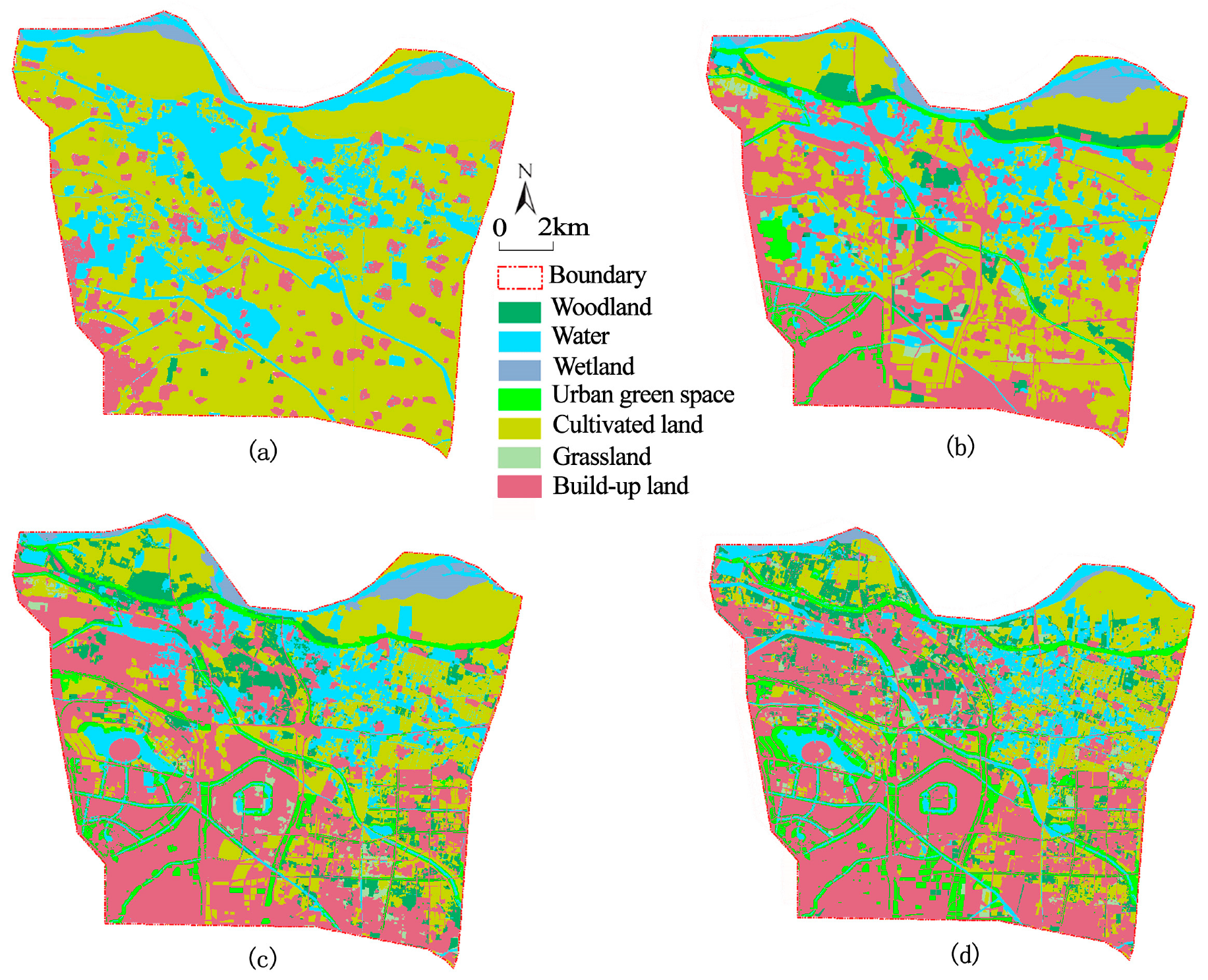
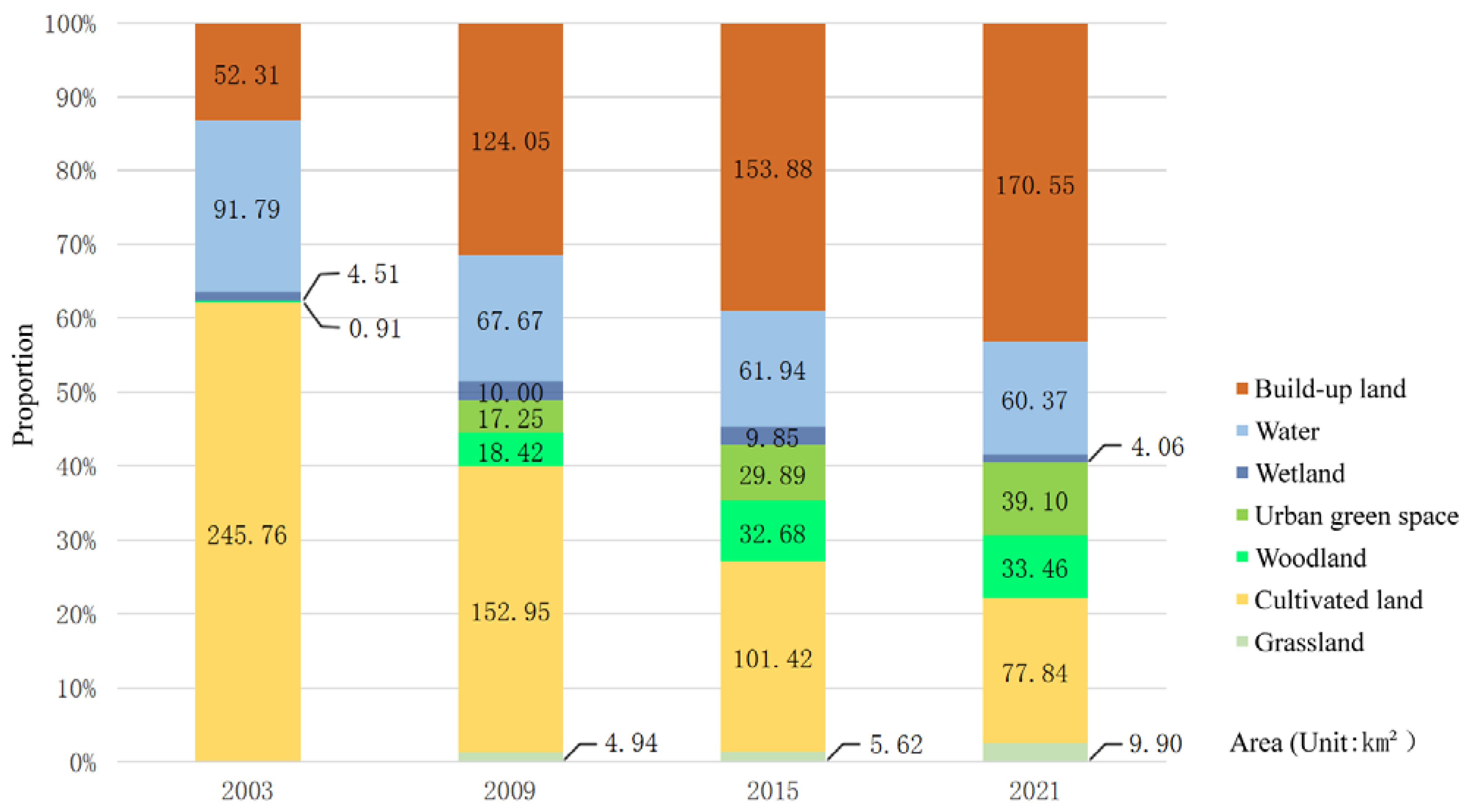
4.1. Characteristics of BGS Changes

4.1.1. Quantitative Changes of BGS from 2003 to 2021

The land use transfer matrix can be obtained by processing land use data with ArcGIS and Excel software using the transition matrix formula (

Table 1. Transition matrix of BGS during the period of 2003–2021 in Zhengdong New District (unit: km²).

Year	Land Use Type	Grassland	Cultivated Land	Woodland	Urban Green Space	Wetland	Water	Built-Up Land	Total
2003–2009	Cultivated land	4.10	131.52	14.97	7.62	3.55	13.28	70.72	245.76
	Woodland	0.00	0.32	0.00	0.13	0.00	0.00	0.46	0.91
	Wetland	0.00	1.81	0.00	0.01	2.19	0.45	0.05	4.51
	Water	0.54	13.04	1.74	6.17	4.24	51.65	14.41	91.79
	Built-up land	0.30	6.40	1.72	3.33	0.00	2.19	38.37	52.31
	Total	4.94	153.09	18.43	17.26	9.98	67.57	124.01	395.28
2009–2015	Grassland	0.92	1.63	0.11	0.10	0.00	0.07	2.11	4.94
	Cultivated land	2.83	80.04	17.17	7.96	0.46	9.90	34.59	152.95
	Woodland	0.34	4.85	7.20	2.07	0.00	0.54	3.42	18.42
	Urban green space	0.00	1.82	0.90	12.12	0.06	1.38	0.97	17.25
	Wetland	0.00	0.70	0.04	0.03	9.23	0.00	0.00	10.00
	Water	0.35	6.11	3.15	2.71	0.01	45.36	9.98	67.67
	Built-up land	1.16	7.06	4.11	4.88	0.00	4.02	102.82	124.05
	Total	5.60	102.21	32.68	29.87	9.76	61.27	153.89	395.28
2015–2021	Grassland	0.17	1.10	0.58	0.42	0.00	0.05	3.30	5.62
	Cultivated land	2.77	55.63	10.53	8.95	0.75	7.19	15.60	101.42
	Woodland	1.09	5.01	15.80	3.88	0.03	0.31	6.56	32.68
	Urban green space	0.20	0.56	0.58	21.27	0.20	5.19	1.89	29.89
	Wetland	0.20	5.05	0.39	0.14	1.02	2.96	0.09	9.85
	Water	1.90	4.89	2.28	0.76	2.02	43.27	6.82	61.94
	Built-up land	3.57	5.60	3.30	3.68	0.04	1.40	136.29	153.88
	Total	9.90	77.84	33.46	39.10	4.06	60.37	170.55	395.28

). The proportional composition, transfer rate of each type of land (Figure 5), and the comprehensive dynamic degree can be calculated. Regarding the overall scale and speed of change, the BGS area reduced from 342.97 km² in 2003 to 224.73 km² in 2021, with an average annual reduction of 6.57 km² and an average annual reduction rate of 1.92%. Cultivated land experienced the most significant decrease of 167.92 km², with a reduced rate of 68.33%, mainly converted to built-up land. The average annual reduction rates of BGS were 3.49% from 2003 to 2009 and 1.43% from 2009 to 2021. This rate was higher before 2009 because of the rough occupation of cultivated lands.

Among the three periods, 2003 to 2009 experienced the highest degree of comprehensive land dynamics at 4.84%, indicating the highest level of land activity. This period experienced a reduction rate of 20.92%, while the built-up land area increased drastically from 52.31 km² to 124.05 km². The reduction rate of the land area of BGS was 20.92%, and the area of built-up land increased dramatically from 52.31 km² to 124.05 km², which became the most significant proportion of land besides cultivated land in 2009. The increased built-up land was mainly transformed from cultivated land and water areas of 70.72 km² and 14.41 km², respectively. This transformation was associated with accelerated urbanisation and growing demand for construction land. Changes in BGS included increased woodland areas, urban green spaces, grasslands, and wetlands from the cultivated land of 14.97 km², 7.62 km², 4.10 km², and 3.55 km², respectively. These changes were attributed to Zhengzhou’s positive response to the national policy of returning cultivated land to woodlands and grasslands since 2002. However, urban green space is growing notably with construction land expansion. This was a period of expansion in which construction activities in Zhengdong New District occupied considerable agricultural resources. A large amount of BGS was converted into built-up land. And the insufficient environmental protection awareness caused a gradual encroachment of the water area.

From 2009 to 2015, the area of BGS that transformed into built-up land was 51.07 km², with a reduction rate of 11%. The transformation rates of grassland, cultivated land, woodland, and water were 42.71%, 22.62%, 18.57%, and 14.75%, respectively. The transferred area was smaller compared to 2003–2009 due to the changes within each type of land, including the demolition of villages into urban building land. The reduction area of cultivated land remains the largest, with the reduction rate of cultivated land decreasing from 37.71% to 33.17% during 2003–2009. The areas of water and wetlands showed a decreasing trend. The reduction area of water became smaller than that during 2003–2009 due to the excavation and storage of Long Lake and Longzi Lake in 2012. The areas of green land and woodland continued to increase by 12.62 km² and 14.26 km², respectively, mainly due to the transfer of cultivated land. The comprehensive dynamic degree of land change decreased to 3.88% during this period.

From 2015 to 2021, the area of built-up land increased by 16.67 km², with an increased rate of 10.83%. This increase was mainly due to the transfer of BGS, such as cultivated land, grassland, and water. A total of 15.38% of the cultivated land was transferred to built-up land. However, the reduction rate of the cultivated land was reduced to 23.25% due to the implementation of the cultivated land protection system of the occupancy–replenishment balance. Benefiting Zhengzhou’s construction of a national central city and development of a greening system of “patches” and “corridors”, urban green space increased steadily with a rate of 30.81%. The transformation area from BGS to built-up land was the lowest among the three periods. And the changes in all the land types were relatively mild. The comprehensive dynamic degree of land change was 3.44%, which was the smallest among the three periods. These results show that the development of new districts aimed at the intensive use of urban land and improving its intrinsic quality in the transformation from rapid urbanisation to high-quality development.

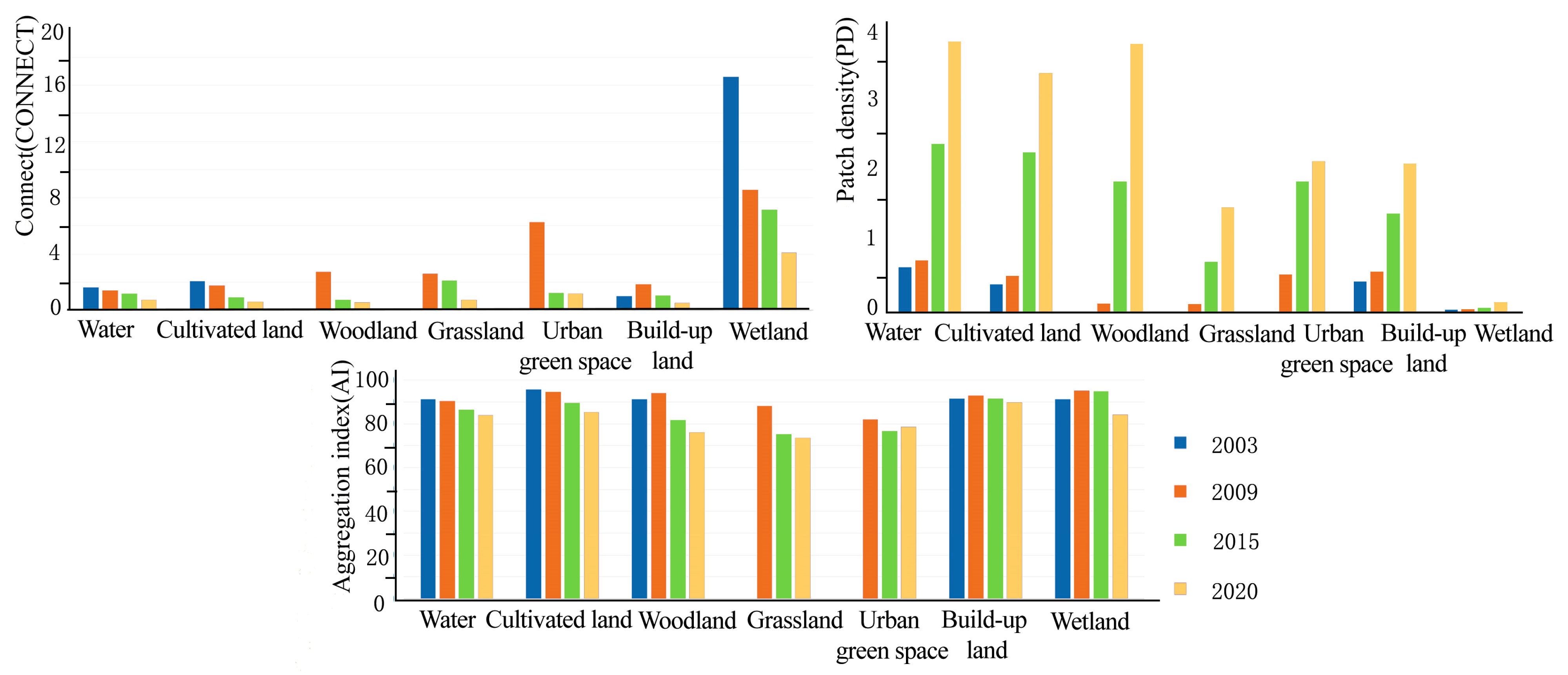
4.1.2. Landscape Indices Changes of BGS from 2003 to 2021

The three landscape pattern indices of patch density (PD), connectivity (Connect), and aggregation index (AI) of various BGS were analysed by combining Arcgis and Fragstats software. The results are shown in Figure 6.

According to the results, the patch density (PD) of both BGS and built-up land increased from 2003 to 2021, indicating an increased number of patches per square kilometre for all land types. The connectivity (Connect) of all types of BGS decreased from 2003 to 2021, indicating that BGS presents a fragmented state. These results imply that construction land expansion dismembered various BGS and led to their fragmentation under accelerated urbanisation.

According to the AI results, the AI of cultivated land, water, and grassland decreased from 2003 to 2021, indicating that the patches were more dispersed and consisted of more small patches. The AI of woodlands and wetlands increased and then decreased, demonstrating the tendency of aggregation and then dispersion. Urban green space fell from 81.6 in 2009 to 77.0 in 2015, while PD increased significantly from 0.5 in 2009 to 1.8 in 2015, illustrating greater urban green space diffusion during this period. From 2015 to 2021, the AI and PD of urban green spaces increased, indicating that urban green spaces evolved more in aggregation than diffusion forces. These evolutions contributed to a more balanced spatial distribution. From 2003 to 2021, the AI of the built-up land first increased and then decreased. Construction land presented a clustered distribution from 2003 to 2009 and then trended to a dispersed distribution with small patches in the following two periods.

4.2. Driving Factors of BGS Changes

Combined with the Pearson correlation analysis results, the correlation coefficient between the population and the BGS area is −0.988. The correlation coefficient between GDP and population is 0.993. And the correlation coefficient between GDP and BGS area is −0.978 (

Table 2. Correlation between socioeconomic factors and spatial variation in BGS.

Factor		Pearson Correlation Coefficient	Significance (Two-Tailed)
Population	GDP	0.993 **	0.001
	BGS area	−0.988 **	0.002
GDP	population	0.993 **	0.001
	BGS area	−0.978 **	0.004
BGS area	population	−0.988 **	0.002
	GDP	−0.978 **	0.004

Note: ** indicates a significant correlation at the 0.01 level (two-tailed).

). The results indicate a significant negative relationship between economic development, population growth, and BGS contraction. Economic development and increased population size contributed to continuous urban expansion, resulting in the inevitable reduction in BGS in Zhengdong New District, including cultivated land, grassland, ponds, and waterways.

Various physical geographic factors, such as distance from the main urban area, major roads, and major rivers, as well as natural conditions like slope, elevation, and water, influence the evolution of BGS to varying degrees. According to the results of the geographic detector (

Table 3. The result of the geographical detector factor.

Drive Factor	Water Area	Slope	Distance from Major Roads	Elevation	Distance from River Systems	Distance from the Main Urban Area
q Statistical	0.23	0.09	0.11	0.16	0.10	0.24
Sig. q	0.07	0.95	0.43	0.02	0.53	0.04

), the explanatory powers for BGS evolution include the distance from the main urban area (0.24), distance from major roads (0.11), and distance from river systems (0.10), slope (0.09), water area (0.23), and elevation (0.16). An explanatory power of less than 0.4 indicates that these physical geographic factors have little impact on the changes in BGS, but there is still some correlation. These factors are ranked as the distance from the main urban area > water area > distance from major roads > elevation > distance from river systems > slope.

5. Discussion

5.1. The Overall Evolution of the “Patch–Corridor–Matrix” Model of BGS

The above results show that the spatial pattern of the “patch–corridor–matrix” has changed dramatically after the anthropogenic disturbance of the new urban district. Combining landscape indices with ecological processes can enhance the scientific validity of examining the evolutionary pattern [29]. Before the 2003 development of Zhengdong New District, the BGS consisted of a large area of agricultural land. The water and ponds were embedded as the original resource-based environmental corridors and patches. In contrast, the spatial pattern artificially stabilised after 2020. This aligns with most major cities’ development paths, where green spaces become increasingly fragmented as cities grow [41].

From 2003 to 2009, the old city expanded northward and eastward along the peripheral Zhongzhou Avenue and National Highway 310, forming the CBD and commercial and residential logistics area. Simultaneously, Longzihu University Park began construction as the centre of the study area. Several new roads, such as highways, expressways, and main roads, were built to divide the matrix into a corridor style. Therefore, the BGS showed the coexistence of marginal contraction, internally filled contraction, and corridor cutting. These changes suggest that the BGS was disturbed in the early stages of constructing the new area, resulting in a considerable change in the “patch–corridor–matrix” model. However, ecological effects remained dominant in the landscape pattern during this period.

From 2009 to 2015, the built-up land showed an overall trend of “large scattering and small concentration”. The built-up land expanded from the CBD to Longhu District. The Longzihu University Park continued to expand. The southeastern Baisha Park presented a dotted status. This trend led to extensive fragmentation of BGS that showed a combined pattern of marginal contraction, internally filled contraction, perforated contraction, and perforated introduction. The stream and the green belt on both sides of the road formed a clear skeleton, and the corridor was almost formed. Overall, the BGS displayed disorganisation and disorderliness during this period.

From 2015 to 2021, all land groups were fully developed, except for the modern agricultural park. The built-up land expanded to a new science and education district in the north and Baisha Park in the east. And the Longzi Lake area was almost built. The results of the AI show that the urban green space, which was artificially introduced as patches, has become more agglomerative at this stage, indicating a tendency towards a state of artificial equilibrium. This change marks the gradual transition of urban development from the “era of increment” to the “era of stock”. The next step should fully use the existing natural ecological space to protect the BGS, for example, via a systematic methodology for planning urban green infrastructure networks to enhance landscape connectivity and reduce green space fragmentation in Detroit [42].

5.2. The Combined Effect of the Four Factors of the “Sustainability Prism” Model

Our results suggest that socioeconomic factors significantly influence the spatial evolution of the BGS compared to physical geography, which differs from the findings of previous macro-scale studies [23,24]. The old city cannot cope with rapid urbanisation’s economic activity and population density. Therefore, new district expansion becomes essential for urban development. It is known from previous studies that BGS is positively correlated with water and elevation and negatively correlated with distance from the central city, major roads, and major rivers. Therefore, BGS susceptible to occupation include areas close to the main urban area, roads and rivers, and areas with flatter topography and higher elevations. While physical geography played a constraining role in this process, it did not change the trend towards large-scale occupation of the BGS. From 1998 to 2021, the population growth rate of Zhengzhou New District was 102.61%, and the GDP growth rate was 1835.03%. Zhengdong New District is the best location for Zhengzhou’s urban expansion due to its proximity to the Zhengzhou National Economic and Technological Development Zone, multiple external transportation, and the relocation of the former Dongjiao Airport. Consequently, the urban expansion inevitably occupied the BGS of Zhengdong New District.

Ecological liveability and economic development are the two main conflicts in the spatial evolution of land use, as sustainable urban development needs to be achieved by preserving environmental resources and economic vitality. Ecological liveability factors drive the value of urban ecological space for rainwater storage. In the detailed conceptual planning of Zhengdong New District, Kisho Kurokawa Architects and the Urban Design Office paid attention to an ecological environment. A spatial structure of clusters was adopted regarding eco-city concepts, such as symbiotic cities, metabolism, and circular cities. The water system and greenery connected these clusters. In these clusters, Ruyi Lake, Long Lake, and Longzi Lake connect the main rivers to the city. Driven by the ecological conservation eco-protection policy for Zhengzhou, the planning for Zhengdong New District is well implemented to form a blue–green network structure of “one screen, five belts, three lakes, and multiple dots”. These plans include the “Zhengzhou National Central City Ecological Construction Master Plan (2016–2025)” and the “Forest Henan Ecological Construction Plan (2018–2027)”. Driven by ecological liveability factors, the urban green space of Zhengdong New District increased from 0 km² to 39.1 km² in 2021, and the length of the river network increased from 98.14 km to 154.68 km. This is similar to the urban development paths of developed countries, such as France and the United States [15,28].

According to the “Zhengzhou Water Chronicle.” [43], Zhengdong New District is located on the alluvial sector plains by the Yellow River, formed by many historical floods and riverway changes. It belongs to the Yellow River Huayuankou Irrigation District and the Yangqiao Irrigation District. The northern area was once pits and fish ponds, so flood safety was a priority. The modern agricultural park in the northeast sits on a prominent low-lying terrain, with almost half of the surface area being pond water and still undeveloped. From 2003 to 2021, dredging, connecting, and expanding the “three rivers and one canal”, namely, the Jinshui River, Qili River, Xiong’er River, and Dongfeng Canal, were carried out to ensure flood safety. This project increased the river network density from 0.25 km/km² to 0.39 km/km². The Long Lake preserves the existing pond surface to the maximum extent, covering an area of about 5.6 km² and storing rainwater with a volume of 1.93 million m³. Rainwater safety factors positively affect artificially introduced patches and corridors. Therefore, Australian academics suggest that a preferable planning process should consider stormwater safety requirements to maximise water-sensitive urban design outcomes [44]. Some Chinese scholars often discuss maximising rainwater storage patches and corridors to achieve rainwater dissipation and land conservation [45]. The watershed pattern evolves from the natural ecological state of large ponds to the “patch + corridor” model, which combines artificial and natural factors. It is crucial to develop policies to optimise the BGS layout for flood safety.

In summary, the BGS was driven by the urban social economy, the impact of physical geography, the promotion of ecological liveability, and the need for flood safety, showing different evolutionary processes (Figure 7). These four factors play different roles as the four vertices of the “sustainability prism model”.

6. Conclusions and Implications

6.1. Conclusions

This study systematically analyses the dynamic changes and evolution mechanism of BGS in Zhengdong New District, filling a crucial gap in research cases regarding BGS within the scale of new urban districts. This exploration combines qualitative and quantitative methods to gain insight into BGS evolution. This study arrived at the following conclusions.

The BGS decreased by 35%, with an average reduction of 6.57 km² over the past 20 years. Cultivated land decreased obviously with a reduction rate of about 68%. The water remained relatively stable. Urban green spaces increased steadily and tended towards a more stable and aggregated state in later years. In addition to urban green spaces, the landscape index of BGS indicated decreased connectivity and aggregation, and increased patch density. The patches were more fragmented and discrete and consisted of more small patches. The BGS spread outward, mainly along the edge of the old city. It showed a combined pattern of marginal contraction, internally filled contraction, perforated contraction, perforated introduction, and corridor cutting. Before 2009, construction activities occupied cultivated lands and other previously uninhabitable areas, and the ecological features of BGS remained predominant. Compared to the first period of rough urban expansion, the following two periods focused more on ecological protection, rainwater safety, and improving the overall urban quality. The spatial–temporal evolution of BGS alternated sequentially among ecological, disorderly, and balanced states.

Multiple factors, including social economy, rainwater safety, ecological liveability, and background conditions, influence the above-mentioned evolutionary pattern. The social economy drives the expansion of built-up land, resulting in significant shrinkage and fragmentation of BGS, with feeble influence from physical geography. The correlation coefficients of the BGS area with population and GDP are −0.988 and −0.978, respectively, whereas the explanatory power of natural and geographical factors is less than 0.4. Furthermore, rainwater safety and ecological liveability factors positively affect spatial development. As one of the major contradictions in urbanisation development, ecological liveability factors inhibit the reduction in BGS. For rainwater safety, the original large northeastern pond and other susceptible areas were preserved in the study area, with additional artificially introduced patches and corridors as rainwater storage spaces.

6.2. Implications

6.2.1. Determining the Optimal Spatial Pattern of the BGS

The spatial pattern of BGS is changing from an ecological state to an artificial “patch–corridor–matrix” state. Understanding its evolutionary patterns is the basis for land use planning. To improve the ecological function of the city, future research should identify direct relationships between the BGS layout and various factors, such as resident health and surface flooding dissipation. Furthermore, establishing evaluation indicators can further quantify the “Sustainable Prism” model. The ultimate objective is to achieve a stable “patch-corridor-matrix” spatial pattern, for example, to protect clustered urban green spaces and increase the BGS’s connectivity.

6.2.2. Assessing the Land Suitability of Undeveloped BGS

The qualitative analysis revealed that rainwater safety is a top priority for Zhengdong New District. The results showed that socioeconomic development played a driving role in accelerating the development of the new district. However, the northern region of the study area has not been fully developed, as outlined in the existing urban master plan. Rainwater safety assessment is necessary for the undeveloped BGS. The suitability evaluation of land development is the basis and premise for preparing territorial spatial planning. Most of the current land suitability evaluations use the factor overlay method. Therefore, the land suitability of the BGS regarding rainwater safety must be evaluated and incorporated into territorial spatial planning.

References

1. Solin, L.; Feranec, J.; Novacek, J. Land cover changes in small catchments in Slovakia during 1990-2006 and their effects on frequency of flood events. Nat. Hazards 2011, 56, 195–214. [Google Scholar] [CrossRef]
2. Hussein, K.; Alkaabi, K.; Ghebreyesus, D.; Liaqat, M.U.; Sharif, H.O. Land use/land cover change along the Eastern Coast of the UAE and its impact on flooding risk. Geomat. Nat. Hazards Risk 2020, 11, 112–130. [Google Scholar] [CrossRef] [Green Version]
3. Zhou, J.J.; Liu, J.H.; Shao, W.W.; Yu, Y.D.; Zhang, K.; Wang, Y.; Mei, C. Effective Evaluation of Infiltration and Storage Measures in Sponge City Construction: A Case Study of Fenghuang City. Water 2018, 10, 937. [Google Scholar] [CrossRef] [Green Version]
4. Sander, H.A.; Zhao, C. Urban green and blue: Who values what and where? Land Use Policy 2015, 42, 194–209. [Google Scholar] [CrossRef]
5. European Environment Agency. Green Infrastructure and Territorial Cohesion; Technical Report No. 18/2011; European Environment Agency: Copenhagen, Denmark, 2011. [Google Scholar]
6. Jiao, X.X.; Zhao, Z.M.; Li, X.; Wang, Z.F.; Zhang, Y.J. Advances in the blue-green space evaluation index system. Ecohydrology 2023, 16, e2527. [Google Scholar] [CrossRef]
7. Yang, G.Y.; Yu, Z.W.; Jorgensen, G.; Vejre, H. How can urban blue-green space be planned for climate adaption in high-latitude cities? A seasonal perspective. Sust. Cities Soc. 2020, 53, 11. [Google Scholar] [CrossRef]
8. Beaugeard, E.; Brischoux, F.; Angelier, F. Green infrastructures and ecological corridors shape avian biodiversity in a small French city. Urban Ecosyst. 2021, 24, 549–560. [Google Scholar] [CrossRef]
9. Ebi, K.L.; Bowen, K. Green and blue spaces: Crucial for healthy, sustainable urban futures. Lancet 2023, 401, 529–530. [Google Scholar] [CrossRef]
10. Nghiem, L.T.P.; Zhang, Y.C.; Oh, R.R.Y.; Chang, C.C.; Tan, C.L.Y.; Shannahan, D.F.; Lin, B.B.; Gaston, K.J.; Fuller, R.A.; Carrasco, L.R. Equity in green and blue spaces availability in Singapore. Landsc. Urban Plan. 2021, 210, 104083. [Google Scholar] [CrossRef]
11. White, M.P.; Alcock, I.; Wheeler, B.W.; Depledge, M.H. Would You Be Happier Living in a Greener Urban Area? A Fixed-Effects Analysis of Panel Data. Psychol. Sci. 2013, 24, 920–928. [Google Scholar] [CrossRef]
12. Zhang, Y.; Jiang, P.; Cui, L.Y.; Yang, Y.; Ma, Z.J.; Wang, Y.; Miao, D.H. Study on the spatial variation of China’s territorial ecological space based on the standard deviation ellipse. Front. Environ. Sci. 2022, 10, 16. [Google Scholar] [CrossRef]
13. Kuller, M.; Reid, D.J.; Prodanovic, V. Are we planning blue-green infrastructure opportunistically or strategically? Insights from Sydney, Australia. Blue-Green Syst. 2021, 3, 267–280. [Google Scholar] [CrossRef]
14. Helming, K.; Perez-Soba, M. Landscape Scenarios and Multifunctionality: Making Land Use Impact Assessment Operational. Ecol. Soc. 2011, 16, 50. [Google Scholar] [CrossRef] [Green Version]
15. Pauleit, S.; Ennos, R.; Golding, Y. Modeling the environmental impacts of urban land use and land cover change—A study in Merseyside, UK. Landsc. Urban Plan. 2005, 71, 295–310. [Google Scholar] [CrossRef]
16. Nor, A.N.M.; Corstanje, R.; Harris, J.A.; Brewer, T. Impact of rapid urban expansion on green space structure. Ecol. Indic. 2017, 81, 274–284. [Google Scholar] [CrossRef]
17. Liu, X.P.; Li, X.; Chen, Y.M.; Tan, Z.Z.; Li, S.Y.; Ai, B. A new landscape index for quantifying urban expansion using multi-temporal remotely sensed data. Landsc. Ecol. 2010, 25, 671–682. [Google Scholar] [CrossRef]
18. Masoudi, M.; Tan, P.Y. Multi-year comparison of the effects of spatial pattern of urban green spaces on urban land surface temperature. Landsc. Urban Plan. 2019, 184, 44–58. [Google Scholar] [CrossRef]
19. Turner, M.G. Landscape ecology in North America: Past, present, and future. Ecology 2005, 86, 1967–1974. [Google Scholar] [CrossRef] [Green Version]
20. Raines, G.L. Description and comparison of geologic maps with FRAGSTATS—A spatial statistics program. Comput. Geosci. 2002, 28, 169–177. [Google Scholar] [CrossRef]
21. Wu, J.; Yang, S.; Zhang, X. Interaction Analysis of Urban Blue-Green Space and Built-Up Area Based on Coupling Model-A Case Study of Wuhan Central City. Water 2020, 12, 2185. [Google Scholar] [CrossRef]
22. Haaland, C.; van den Bosch, C.K. Challenges and strategies for urban green-space planning in cities undergoing densification: A review. Urban For. Urban Green. 2015, 14, 760–771. [Google Scholar] [CrossRef]
23. Wang, D.; Fu, J.Y.; Xie, X.L.; Ding, F.Y.; Jiang, D. Spatiotemporal evolution of urban-agricultural-ecological space in China and its driving mechanism. J. Clean Prod. 2022, 371, 9. [Google Scholar] [CrossRef]
24. Hu, Y.F.; Zhang, Y.Z. Spatial-temporal dynamics and driving factor analysis of urban ecological land in Zhuhai city, China. Sci. Rep. 2020, 10, 16174. [Google Scholar] [CrossRef]
25. Xu, Z.; Zhang, Z.; Li, C. Exploring urban green spaces in China: Spatial patterns, driving factors and policy implications. Land Use Policy 2019, 89, 104249. [Google Scholar] [CrossRef]
26. Meyfroidt, P.; Lambin, E.F.; Erb, K.H.; Hertel, T.W. Globalization of land use: Distant drivers of land change and geographic displacement of land use. Curr. Opin. Environ. Sustain. 2013, 5, 438–444. [Google Scholar] [CrossRef]
27. Ju, X.; Xinhui, J.; Weifeng, L.; Liang, H.; Junran, L.; Lijian, H.; Jingqiao, M. Ecological redline policy may significantly alter urban expansion and affect surface runoff in the Beijing-Tianjin-Hebei megaregion of China. Environ. Res. Lett. 2020, 15, 1040b1. [Google Scholar] [CrossRef]
28. Thomas, H.; Gaetan, P.; Roberta, R.; Hugues, B.; Jacques, B.; Xavier, P.; Jean-Baptiste, N.; Manuel, A.M.J.; Stefano, B.; Cendrine, M.; et al. European blue and green infrastructure network strategy vs. the common agricultural policy. Insights from an integrated case study (Couesnon, Brittany). Land Use Policy 2022, 120, 13. [Google Scholar] [CrossRef]
29. Forman, R.T.T. Some general principles of landscape and regional ecology. Landsc. Ecol. 2010, 10, 133–142. [Google Scholar] [CrossRef]
30. Godschalk, D.R. Land use planning challenges—Coping with conflicts in visions of sustainable development and livable communities. J. Am. Plan. Assoc. 2004, 70, 5–13. [Google Scholar] [CrossRef]
31. Forman, R.T.T.; Godron, M. Landscape Ecology; John Wiley: New York, NY, USA, 1986; p. 195. [Google Scholar]
32. Zaccarelli, N.; Riitters, K.H.; Petrosillo, I.; Zurlini, G. Indicating disturbance content and context for preserved areas. Ecol. Indic. 2008, 8, 841–853. [Google Scholar] [CrossRef]
33. Jiao, S.; Zhang, X.L.; Xu, Y. A review of Chinese land suitability assessment from the rainfall-waterlogging perspective: Evidence from the Su Yu Yuan area. J. Clean Prod. 2017, 144, 100–106. [Google Scholar] [CrossRef]
34. Chapin, F.S., Jr.; Kaiser, E.J.; Godschalk, D.R. Urban Land Use Planning; University of Illinois Press: Champaign, IL, USA, 2009; p. 195. [Google Scholar]
35. Guan, D.J.; Li, H.F.; Inohae, T.; Su, W.C.; Nagaie, T.; Hokao, K. Modeling urban land use change by the integration of cellular automaton and Markov model. Ecol. Model. 2011, 222, 3761–3772. [Google Scholar] [CrossRef]
36. Shen, G.; Yang, X.C.; Jin, Y.X.; Luo, S.; Xu, B.; Zhou, Q.B. Land Use Changes in the Zoige Plateau Based on the Object-Oriented Method and Their Effects on Landscape Patterns. Remote Sens. 2020, 12, 14. [Google Scholar] [CrossRef] [Green Version]
37. Uuemaa, E.; Mander, U.; Marja, R. Trends in the use of landscape spatial metrics as landscape indicators: A review. Ecol. Indic. 2013, 28, 100–106. [Google Scholar] [CrossRef]
38. Zhou, Y.; Zhang, Q.; Singh, V.P.; Xiao, M.Z. General correlation analysis: A new algorithm and application. Stoch. Environ. Res. Risk Assess. 2015, 29, 665–677. [Google Scholar] [CrossRef]
39. Wang, J.F.; Li, X.H.; Christakos, G.; Liao, Y.L.; Zhang, T.; Gu, X.; Zheng, X.Y. Geographical Detectors-Based Health Risk Assessment and its Application in the Neural Tube Defects Study of the Heshun Region, China. Int. J. Geogr. Inf. Sci. 2010, 24, 107–127. [Google Scholar] [CrossRef]
40. Chin, C.H.; Lo, M.C. Rural tourism quality of services: Fundamental contributive factors from tourists’ perceptions. Asia Pac. J. Tour. Res. 2017, 22, 465–479. [Google Scholar] [CrossRef] [Green Version]
41. Fahrig, L. Effects of habitat fragmentation on biodiversity. Annu. Rev. Ecol. Evol. Syst. 2003, 34, 487–515. [Google Scholar] [CrossRef] [Green Version]
42. Zhang, Z.; Meerow, S.; Newell, J.P.; Lindquist, M. Enhancing landscape connectivity through multifunctional green infrastructure corridor modeling and design. Urban For. Urban Green. 2019, 38, 305–317. [Google Scholar] [CrossRef]
43. Zhengzhou Water Authority. Zhengzhou Water Chronicle; The Yellow River Water Conservancy Press: Zhengzhou, China, 2015; pp. 138–222. [Google Scholar]
44. Coyne, T.; Zurita, M.D.M.; Reid, D.; Prodanovic, V. Culturally inclusive water urban design: A critical history of hydrosocial infrastructures in Southern Sydney, Australia. Blue-Green Syst. 2020, 2, 364–382. [Google Scholar] [CrossRef]
45. Zhou, K.J.; Jiao, S.; Han, Z.W.; Liu, Y.C. Assessment of flood regulation service based on source-sink landscape analysis in urbanized watershed. River Research and Applications; Wiley: Hoboken, NJ, USA, 2022. [Google Scholar] [CrossRef]
Figure 1. Evolution of BGS in a new urban district: (a) Pre-development status of new urban district; (b) Post-development status of new urban district; (c) Spatial evolution patterns of BGS during the development of new urban district.
Water 15 02417 g001
Figure 2. Application of the “sustainability prism” model: (a) “Sustainability prism” model in land use planning; (b) Application of “sustainability prism” model in the driving factors of BGS.
Water 15 02417 g002
Figure 3. The basic information of Zhengdong New District: (a) Geographical location; (b) Functional zoning; (c) Current land-use in 2021.
Water 15 02417 g003
Figure 4. Spatial evolution of BGS in the study area from 2003 to 2021: (a) 2003; (b) 2009; (c) 2015; (d) 2021.
Water 15 02417 g004
Figure 5. Area and proportion of each land type from 2003 to 2021 in Zhengdong New District.
Water 15 02417 g005
Figure 6. Landscape index of each land type from 2003 to 2021 in Zhengdong New District.
Water 15 02417 g006
Figure 7. Dynamic spatial evolution of BGS in the study area.
Water 15 02417 g007