1. Introduction
During the last two centuries, the exploitation of the water resources has increased many folds as a consequence of industrialization, urbanization, population growth and climate change [
1,
2]. This has resulted in increased dependency on the groundwater for domestic, industrial, and irrigational uses [
3,
4,
5]. Therefore, the monitoring of groundwater quality is an important aspect of the management of water resources, especially in the countries such as Saudi Arabia where the groundwater is depleting continuously [
6,
7,
8,
9]. In the countries of arid and semi-arid regions, the surface water resources are scanty, and dependency on groundwater is high; hence, the depletion and degradation of groundwater is very high in these countries [
10,
11]. Moreover, concern over groundwater quality has grown in several parts of the world due to the contamination of groundwater by natural and anthropogenic factors as well as its overexploitation [
12,
13]. Hence, it is essential to monitor and evaluate the quality of groundwater for its sustainable management and protection from degradation [
13,
14].
Various conventional and advanced techniques have been developed for evaluating groundwater quality, including statistical analysis and the use of geographic information systems (GIS) [
15,
16,
17]. These techniques enable the assessment of different water quality parameters and their spatial distribution. However, when the number of water quality parameters is large, it becomes necessary to integrate physicochemical water characterization into a single parameter that describes water quality. The first effort to evaluate water quality using an index was performed by [
18]. Since then, several indices have been developed, including the United States National Sanitation Foundation Water Quality Index (NSFWQI), Bureau of Indian Standard (BIS), Florida Stream Water Quality Index (FWQI), Canadian Water Quality Index (CWQI), and National Water Quality Standards for Malaysia (INWQS) [
19]. Initially, water quality study and prediction relied on mechanism models that analysed the evolution of water body mechanisms [
20]. Subsequently, data-driven models based on statistical approaches such as frequency ratio, fuzzy logic, and evidential-belief function were developed for groundwater quality monitoring and prediction [
21,
22]. However, these data-driven statistical models have drawbacks such as longer anticipation and assessment times, as well as inconsistent results [
23]. To overcome these limitations, researchers turned to nonphysical models based on artificial intelligence (AI), significantly enhancing the accuracy of water quality monitoring and prediction [
19,
23,
24].
The main advantage of AI is its ability to handle complex, nonlinear structures and big datasets at diverse scales, enabling prompt creation of water quality index (WQI) values [
19,
24]. AI-based machine learning (ML) and deep learning (DL) models are utilized in water quality monitoring because they can predict complex phenomena, handle enormous datasets of varying sizes, and are unaffected by missing data [
25,
26]. Over the past 20 years, the use of AI approaches has expanded across various fields. In the context of simulating and predicting water quality, various machine learning algorithms, including adaptive boosting (Adaboost) [
24], gradient boosting (GBM) [
25], extreme gradient boosting (XGBoost) [
26], decision tree (DT) [
27], extra trees (ExT) [
28], radial basis function (RBF) [
29], artificial neural network (ANN) [
29,
30], random forest (RF) [
31], deep feed-forward neural network (DFNN) [
23], and convolutional neural network (CNN) [
22] have been examined for their efficacy. However, researchers still face the challenge of determining the most suitable techniques for a given problem. In this study, we chose to use gradient boosting (GBM), generalized linear model (GLM), deep neural network (DNN), their ensemble stacking, and CNN to achieve the best possible performance with the available nonlinear water quality data from 122 sites.
Existing models for predicting WQI have demonstrated certain limitations, and our chosen model overcomes these shortcomings while providing additional benefits. Firstly, when dealing with highly nonlinear data such as hydrologic and climatic data, some ML models can suffer from under- and overfitting, resulting in suboptimal performance [
31]. In contrast, our approach incorporates ensemble stacking and CNN models, which were specifically chosen to address these limitations. By combining weak and strong ML and DL algorithms, our ensemble stacking model can more accurately learn highly nonlinear data, leading to improved prediction results [
32]. Additionally, DL models, while effective at learning noisy and highly nonlinear data, typically require a large amount of data to achieve optimal performance [
33,
34]. However, we tackle this limitation by implementing hyperparameter optimization techniques.
The benefits of utilizing these chosen models and optimizing their hyperparameters are twofold. Firstly, we can overcome the under- and overfitting issues often encountered by traditional ML models, ensuring a more accurate representation of the underlying nonlinear relationships in the data. This leads to improved WQI prediction performance compared to existing models [
31]. Secondly, by leveraging the power of DL models and the ensemble stacking approach, we can effectively capture the complex and intricate patterns present in water quality data, resulting in better prediction outcomes. The utilization of CNN allows us to exploit the spatial and temporal features present in the data, which is especially valuable in the context of water quality monitoring [
22]. Moreover, our emphasis on hyperparameter optimization ensures that we fine-tune the models to achieve optimal performance. By systematically exploring and adjusting the hyperparameters of each model, we aim to enhance their predictive capabilities and maximize their efficacy in capturing the inherent characteristics of the water quality data.
In recent years, the “black-box” nature of many ML and DL models has been a significant research issue, as they provide output without revealing the inner workings of the model. While the output of these models can be useful, it may not always provide reliable measures for decision-making in real-world applications. To address this limitation and propose effective strategies, it is crucial to understand the prediction procedure and how the input variables impact the output. This information is not only important for management purposes but also for gaining a better understanding of the model’s behaviour.
The recent discovery of explainable artificial intelligence (XAI) has provided a solution to this problem. XAI allows researchers to gain insights into how ML or DL models process data and make predictions. By utilizing XAI techniques, researchers can extract more information from the model and acquire a deeper understanding of the decision-making process. This, in turn, leads to more reliable and transparent results, which are essential for making informed decisions in various real-world applications. Therefore, in this research, we applied XGBoost-based SHAP as a technique for XAI in water quality management to extract more information. The objectives of this study are twofold. Firstly, we aim to accurately predict WQI using standalone ML models such as gradient boosting, generalized linear model, deep neural network, hybrid ensemble stacking model, and convolutional neural network, even under limited datasets, by fine-tuning their hyperparameters for optimal performance. Secondly, we employ the technique of XAI by utilizing XGBoost-based SHAP to gain insights into how ML or DL models process data and make predictions.
This study contributes to the research field of water quality monitoring by exploring the efficacy of different ML and DL techniques for predicting WQI, including some of the most recent algorithms. Additionally, this study addresses the challenge of determining the most suitable technique for a given problem, a crucial issue in the field. Moreover, this study introduces the use of XAI techniques, specifically XGBoost-based SHAP, to gain insights into how the model processes data and makes predictions, which is a relatively new concept in the field of water quality management. By leveraging XAI techniques, our research aims to extract valuable information from the models, enhance transparency, and provide a more comprehensive understanding of the prediction outcomes. These insights will facilitate informed decision-making in various real-world applications, contributing to improved water quality management strategies.
2. Materials and Methods
2.1. Study Area
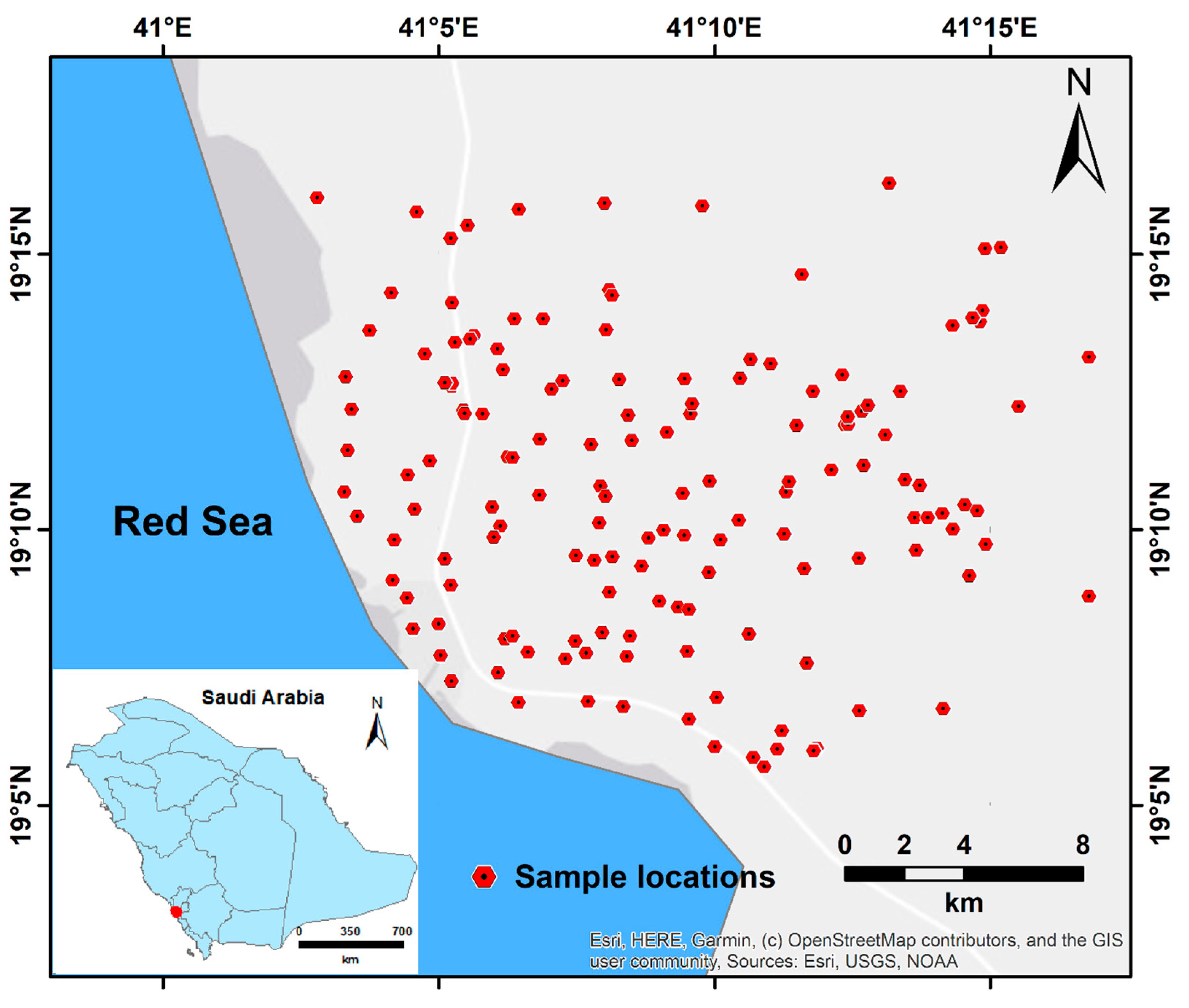
The Red Sea Hills are a prominent outcrop along the Red Sea coastal plain and are composed mostly of Neoproterozoic volcanic-sedimentary rock formations (550–900 Ma). The crystalline basement is covered by broad sedimentary strata from the Cambrian to the present that are not conformable. Al Qunfudhah is located in southwestern Saudi Arabia, on the eastern coastal plain of the Red Sea, and is part of the parallel-running Asir mountain range (
Figure 1). The region has the highest annual average precipitation (AAP) in Saudi Arabia (400–700 mm year
−1) [
35]. Al Qunfudhah and its environs (294 km
2) are among the many cities that fill the Red Sea coastal plain, with a population of approximately 300,000. Through the drainage system, all the precipitation that falls in the high mountains of Asir finally reaches the coastal plain [
36]. The vast majority of the coastal plain is covered by sedimentary strata and friable deposits, which rest above a complex basement that dips roughly westward toward the Red Sea. Consequently, a significant volume of runoff water is able to permeate these sediments and collects in the basement surface basins [
35]. Several communities, including Al Qunfudhah and its surroundings (population: 300,000; area: 294 km
2), are located in the Red Sea coastal plain, which may lead to contamination of the groundwater supply.
2.2. Sample Collection and Processing
The water sample was collected in such a way that it covers almost all parts of the Al Qunfudhah region. The samples were collected from the existing borewells in the region during March and April months of 2022. For calculating the dissolved materials in water, the samples were kept in sealed 2 L polyethylene terephthalate (PET) bottles at 4 degrees Celsius in the dark (P). Each container was labelled with name, the coordinates of the location from where the water was collected, and the sample collection date. All analyses followed the American Public Health Association’s (APHA) standard technique and guide handbook for water and wastewater (CPCB) analysis. We were able to take instantaneous readings of key physicochemical variables and total dissolved solids using a water analyser kit. Overall, we collected and used fourteen water quality parameters, such as total dissolved solids (TDS), electrical conductivity (EC), turbidity (Turb), pH, iron (Fe), total hardness (TH), chloride (Cl), nitrate (NO3), sulfate (SO4), manganese (Mn), copper (Cu), zinc (Zn), chromium (Cr) for further research and WQI calculation.
2.3. Missing Data Treatment Using Random Forest
In statistical analysis, the problem of missing values is regarded as one of the most important concerns. It may significantly affect the analysis and the outcomes of this research. To tackle the problem of missing values, a number of imputation techniques are applied. Imputation is a usual procedure applied to tackle the missing values in a statistical data series. Further, the ML models such as random forest (RF), KNN, and others are also being used for the treatment of missing values [
37]. The use of a random forest for data imputation is a creative and successful imputation technique that possesses almost all of the best imputation techniques’ best qualities. Random forests are fairly good at scaling to large datasets, and they can deal with outliers and nonlinearity in the data. For RF missing data imputation, three general techniques were used:
- (a)
Pre-impute the data, breed the forest, use the closeness of the data, update the initial missing values, iterate to achieve better results.
- (b)
Impute the data while expanding the forest, iterate for better outcomes.
- (c)
Pre-impute the data, build a forest using each variable’s missing values one at a time, use the forest to anticipate the missing values, iterate to achieve better outcomes.
The detailed procedure of missing data imputation using a random forest is given in [
37].
Table 1 provides statistics on various water quality parameters, including TDS, EC, turbidity, pH, Fe, TH, Cl, NO
3, SO
4, Mn, Cu, Zn, Cd, Cr, and WQI. TDS and EC have the highest means and standard deviations, indicating high variability and salinity in the water samples.
2.4. Entropy-Based Groundwater Quality Index Computation
The entropy-based water quality index or entropy-water quality index (EWQI) is an enhanced version of the water quality index (WQI) of Horton [
18]. The entropy model was first introduced by Shannon showing that the amount of information and information entropy are the two key characteristics of this theory [
38]. This strategy significantly minimizes the likelihood of the bias that is frequently brought about by the assignment of parameter weights. The EWQI is considered as an unbiased, precise, consistent, and most robust index and has been utilised for the analysis of water quality across the globe [
17,
39,
40]. The calculation of EWQI involves five steps. In the first step, the information entropy (
ej) is determined using Equation (1).
where
n refers to the number of samples, while
Pij refers to the probability of incidence of the parameter
j’s normalised value expressed as Equation (2).
Suppose
y samples of water (
i = 1, 2, 3…
n) are present, on which
x number of parameters (
j = 1, 2, 3…
n) has to be tested to examine the quality of water, the sample’s ratio of the index values of
j and
i is then provided as Equation (3).
Each parameter’s entropy weight (
wj) was determined using Equation (4) as follows:
In the next step, the quality rating scale (
qj) of the parameters in each sample is calculated using Equation (5).
where
Cj represents the parameter concentration in each water sample, while
Sj represents each parameter’s measured standard in water samples.
Finally, the EWQI is calculated using Equation (6).
2.5. Feature Selection Techniques for Identifying the Most Important Parameters
2.5.1. Recursive Feature Elimination (RFE)
RFE is a feature selection technique that uses the accuracy of a model to identify the most important features. The basic idea behind RFE is to recursively remove the least important features from the dataset while building the model on the remaining features. This process is repeated until a pre-determined number of features is reached. When using RFE with XGBoost, the accuracy of the model is used as a measure to evaluate the importance of each feature. The XGBoost algorithm is trained on the entire dataset, and the feature importance values are determined using the built-in feature importance function. The feature with the lowest importance score is removed from the dataset, and the process is repeated until the desired number of features is reached.
Cross-validation is used to evaluate the performance of the model with different feature sets. It helps to avoid overfitting and to achieve better generalisation of the model. In summary, RFE with XGBoost and cross-validation is a powerful feature selection method, as it makes it possible to identify the most important features in the dataset while evaluating the performance of the model with different feature sets, which helps to avoid overfitting and achieve better generalisation of the model.
2.5.2. Random Forest (RF)
RF is an ensemble learning method that is often used for feature selection because it provides an easy way to determine the importance of features. The basic idea behind the random forest is to train several decision trees on different subsets of the data and then average the results to obtain a final model. When you use a random forest to select features, the feature values are calculated by taking the average of the feature values of all the decision trees in the forest. For each feature, a feature importance is calculated that represents the average decrease in fuzziness (e.g., Gini fuzziness or information gain) when that feature is used to partition a node in the decision trees.
2.5.3. Boruta
Boruta is a feature selection algorithm that uses the concept of “shadow features” to determine the importance of features in a dataset. It is a feature selection method which means that it aims to select all relevant features and reject all irrelevant and redundant features. Boruta uses random forest as its underlying algorithm and can therefore be used with any type of data, including continuous, ordinal, categorical, and binary data. It can also work with both classification and regression problems.
In summary, Boruta is a method for selecting all relevant features that uses the concept of “shadow features” to determine the importance of features in a dataset. It is a powerful and efficient method that can be used for any type of data and for both classification and regression problems.
2.6. Prediction of EWQI Using Machine Learning, Proposed Stacking Model and Deep Learning Model
We used GBM, GLM, and DNN as standalone model to predict EWQI for this study. Then, we used the mentioned three models as a base model and DNN model as a meta-leaner to create a hybrid model such as stacking model. Moreover, we used CNN model to predict WQI to compare the performance with standalone and hybrid models.
In this study, we utilized various ML and DL models, which involved several stages, including data normalization, data splitting, feature selection, model training, model optimization, and model validation.
2.6.1. Data Normalization
This approach involves scaling the input data to ensure that all features have equal importance in the model. Without normalization, features with large values can dominate the model and skew the predictions. In this case, the StandardScaler normalization method was used to scale the data. This method scales the data in such a way that the mean is 0, and the standard deviation is 1. Normalization helps to reduce the impact of outliers and to make the model more stable and robust.
2.6.2. Data Splitting
This approach involves dividing the available data into two sets: training data and testing data. The model is trained on the training data, and its performance is evaluated using the testing data. This approach helps to evaluate the generalization ability of the model and prevent overfitting. In this case, an 80–20 ratio was used for training and testing, which is a commonly used ratio for machine learning [
41].
2.6.3. Feature Selection
The details of feature selection are described in the previous
Section 2.5.
2.6.4. ML and DL Models Used for WQI Prediction
The theoretical background of the models used for predicting WQI is given below:
Gradient Boosting Machine (GBM)
GBM is an ensemble tree-based model which combines several decision trees using a gradient-based optimization as well as boosting algorithms [
41,
42]. It causes an improvement in the performance of model in prediction [
43]. In prediction models, the datasets are separated into various groups using single decision tree model [
44], but in GBM, a sequence of multiple decision trees are built iteratively through the GBM to minimize the loss (error between actual and predicted data) [
45]. The mathematical foundation and resampling procedure details of GBM were presented by Friedman [
46,
47].
Generalized Linear Model (GLM)
The GLM is an advanced version of the most widely used linear regression model. It provides a comprehensive function that can handle datasets for regression analysis that are both linear and nonlinear [
48,
49]. It creates the output model using the exponential family. By maximizing the log-likelihood, the model can be estimated over the parameter vector of the observations [
50]. Although, GLM is an easy model, it has been widely applied for the analysis and prediction of WQI in different parts of the world. Thus, in the current study, the GLM was applied for the prediction of water quality in the Al Qunfudhah region of Saudi Arabia.
Dense Neural Network (DNN)
Due to its greater accuracy, capacity to handle big and nonlinear datasets, training stability, ability to address complicated nonlinear problems, and hierarchical feature selection, the DL method has recently garnered significant prominence over ML techniques [
51,
52,
53]. A multi-layer feed-forward DL architecture was employed in this research in the context of H
2O [
50]. This technique employs a structure similar to that of a typical multilayer perceptron (MLP). Each neuron computed the weights of the input parameters, which were then transmitted to the next neuron through a transfer function [
50]. This model is made up of three levels: an input layer, many hidden layers, and an output layer. The H
2O framework is a powerful artificial neural network that optimizes backpropagation (stochastic gradient decent). In this study, the DL algorithm in the H
2O framework was tailored to the training data using the random grid search approach with 5-fold cross-validation.
CNN
A CNN is a sort of neural network that uses convolutions to extract patterns from data with the goal of developing filters that obtain the most relevant characteristics from the input to accomplish a given job [
54,
55,
56]. As a result, by learning from the data pattern, this algorithm can recognise and resize new items automatically [
55]. As a consequence, researchers have dubbed this method the “object-recognition organisms”, which perform object detection and picture categorization. However, the CNN algorithm’s design differs from that of other neural networks in that it includes a convolutional layer as well as a pooling layer [
57]. These layers may significantly lower the original network’s complexity and the vast number of parameters, allowing for more efficient forward propagation. The convolution kernel of the convolution layer can identify the local time characteristic of the data by sliding the window, and the weights can be determined from the sliding convolution kernel [
57]. Furthermore, the pooling layer is employed to reduce dimensionality by abstracting the various feature extractions using numerous convolution kernels. Finally, the global feature was created by combining local characteristics via the use of completely linked layers. The CNN model is often used for spatial and geometric feature extraction from two- and three-dimensional input data, although it also works well with one-dimensional data. As a result, the one-dimensional convolutional layer should be employed to execute this one-dimensional CNN model. Previous studies employed this 1D CNN model effectively and attained greater accuracy [
58,
59,
60,
61]. Because our data format is one-dimensional, we employed a 1D CNN model in this investigation.
Proposed Stacking Framework
In this study, the stacking framework based on DL model was proposed for forecasting the WQI in the Saudi Arabia’s Al Qunfudhah region. The stacking framework combines numerous learning algorithms in two different ways, making it a type of robust ensemble learning algorithm [
62]. Many different research domains have successfully used the stacking ensemble approach [
63,
64,
65,
66]. Stacking begins with the implementation of multiple ML algorithms to predict the target variables, known as a base learner (level-0), and then the predictions of multiple ML algorithms are integrated by another ML algorithm, known as meta-learner (level-1). In this study, we used GBM, GLM, and DL as base learners (level-0) and combined all algorithms with DL as a meta-learner (level-1).
2.6.5. Model Calibration
This approach involves adjusting model parameters to optimize model performance based on the provided data. In this study, we used grid search algorithm under H2O framework to optimize the hyperparameters of GBM, GLM, and DNN models to obtain the optimal values. In the case of CNN model, we tune the hyperparameters using Bayesian optimization model. The scikit-optimize library’s gp_minimize function uses a Gaussian process (GP) surrogate model to approximate the objective function and suggests new points to evaluate based on Bayesian optimization. The algorithm starts with a set of randomly selected points and fits a GP model to the evaluated points. It then selects the next point based on an acquisition function that balances between exploiting the current best estimate and exploring less certain regions of the search space. This process continues until the maximum number of allowed evaluations is reached, or the minimum threshold is reached. The result is the set of hyperparameters that minimize the objective function, subject to the search space constraints.
2.6.6. Evaluation of the Models
In the context of validating a model for predicting WQI, six metrics can be used to determine the accuracy and precision of the model’s predictions and to compare the performance of different models. RMSE (root mean square error), MAE (mean absolute error), MAPE (mean absolute percentage error), RMSLE (root mean squared logarithmic error), R2 (coefficient of determination), and adjusted R2 are all common metrics for evaluating the performance of a predictive model.
RMSE is a measure of the difference between predicted values and actual values, where the differences are squared and averaged before taking the square root. A lower RMSE value indicates better performance. MAE is similar, but without squaring the differences. A lower MAE value indicates better performance. MAPE measures the average percentage difference between predicted and actual values. A lower MAPE value indicates better performance. RMSLE is similar to RMSE but is calculated on the logarithm of the predicted and actual values. A lower RMSLE value indicates better performance. R2 measures how much of the variance in the actual values is explained by the model’s predictions. Adjusted R2 is a modified version of R2 that accounts for the number of variables used in the model. A higher R2 and adjusted R2 value indicates better performance.
2.7. Improvement in Decision-Making by Integrating WQI Prediction and Explainable Artificial Intelligence (XAI)
Decision-making is a crucial aspect of water resource management, and the accuracy of decision-making depends on the quality of the information on which it is based on. water quality index (WQI) prediction is a tool that helps to assess the overall quality of water in a given region. Conventional methods of WQI prediction, such as statistical and empirical models, have limitations in terms of accuracy and interpretability.
Deep learning, on the other hand, is a subfield of machine learning that uses artificial neural networks to model complex relationships between inputs and outputs [
67]. Deep learning algorithms can process large amounts of data and identify patterns and relationships that are difficult for human analysts to recognise. Using deep learning for WQI prediction can significantly improve the accuracy of decision-making compared to traditional methods. However, the black-box nature of deep learning models can limit the interpretability of the results and make it difficult to understand the underlying relationships between inputs and outputs.
XAI is a branch of AI that aims to create models that are transparent and interpretable, yet have high accuracy [
68]. XAI methods, such as rule-based systems and decision trees, can provide insights into the decision-making process, making it easier to understand the relationships between inputs and outputs. The use of deep learning for WQI prediction in combination with XAI can significantly improve the accuracy and interpretability of decision-making in water resource management. XAI provides a way to make deep learning models more transparent and understandable, so that decision-makers can better understand the relationships between inputs and outputs and make informed decisions based on this knowledge.
In this research, SHAP (SHapley Additive exPlanations) is a popular XAI method based on XGBoost. XGBoost is a gradient boosting algorithm that is widely used for machine learning tasks, including classification and regression problems. SHAP values provide a way to understand the contributions of each feature to the prediction made by XGBoost. SHAP values are based on the Shapley value, a well-established mathematical concept in game theory, and they measure the contribution of each feature to the prediction. The SHAP values are interpretable and provide a clear explanation of the decision-making process, making it easier for the decision-makers to understand the relationships between inputs and outputs.
3. Results
3.1. Missing Value Treatment Using Random Forest
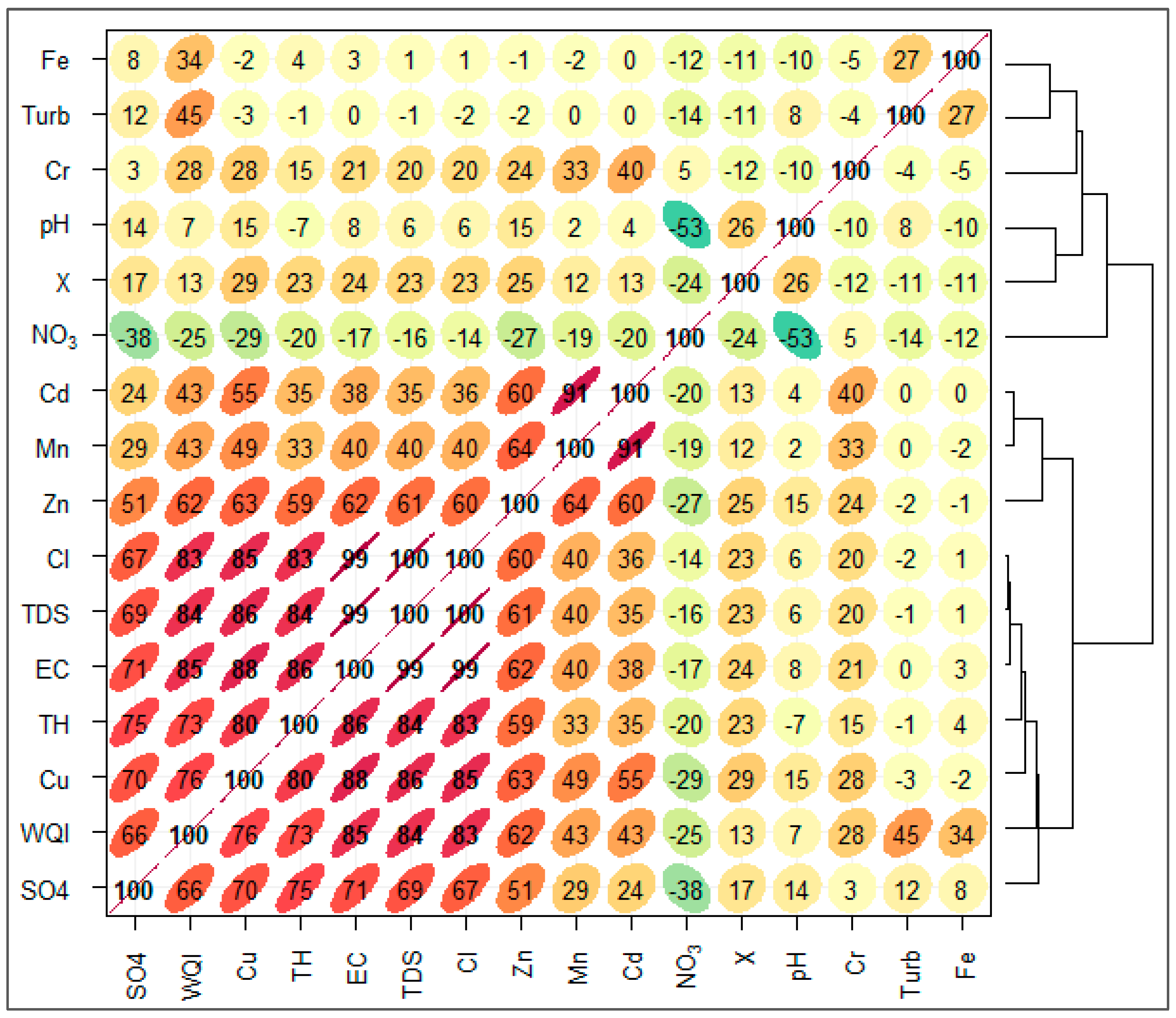
The problem of missing value is very common in hydrogeological research. In this study, the water samples were collected from a large number of sites, and hence the dataset may have some missing values. To check whether the data have some missing values, we visualized the whole data using the heat map in
Figure 2. It shows that the samples such as sulphate (SO
4), manganese (Mn), copper (Cu), zinc (Zn), cadmium (Cd), and chromium (Cr) had missing values of nearly 49%. Thus, we implemented the Rf algorithm for the imputation of missing values from the dataset. After the imputation, the dataset was again visualized, and it was found that there were no more missing values in the data (
Supplementary Figure S1). Finally, the dataset generated after the imputation was used for further analysis in this research.
3.2. Entropy-Based Groundwater Quality Index Computation
In this study, fifteen physiochemical and metal parameters of the groundwater water are used to calculate and predict the WQI. The laboratory analysis of physicochemical and metal properties reveals considerable insights of groundwater water quality. In this study, we identified the parameters that are most responsible for the deterioration of water quality using the entropy analysis. This study revealed that turbidity (0.143) has the maximum weightage for estimating the WQI, followed by Fe (0.128), Mn (0.127), Cd (0.11), and Cl (0.07), while the minimum weightage was observed in pH (0.004), followed by NO3. Therefore, it can be concluded that only a few samples have an acceptable limit for turbidity and Fe, and Mn causes a lower average value, indicating polluted water quality. The maximum values of these parameters are far from the WHO drinking water standards, indicating contamination of groundwater water by pollutants. However, the calculated WQI shows that the present is characterised by a minimum WQI value of 90.75 and a maximum WQI value of 145.29, with an average value of 112.62 (
Figure 2). Yadav et al. (2010) classified the WQI values into five levels: excellent (0–25), good (26–50), poor (51–75), very poor (76–100), and unsuitable (above 100). When we compared our WQI result with the classification scheme of Yadav et al. (2010), we found that most of the samples in this study are classified as very poor, while some of the samples have an unsuitable WQI. Therefore, this is a threat to aquatic ecology and requires urgent monitoring and management. Moreover, the correlation between parameters and WQI showed that TDS, turbidity, Mn, Cd, Cl, Zn, Cu, and TH have strong correlation with WQI, which indicates their influence on the WQI.
3.3. Implementation of Machine Learning and Deep Learning Models for Predicting WQI
3.3.1. Feature Selection
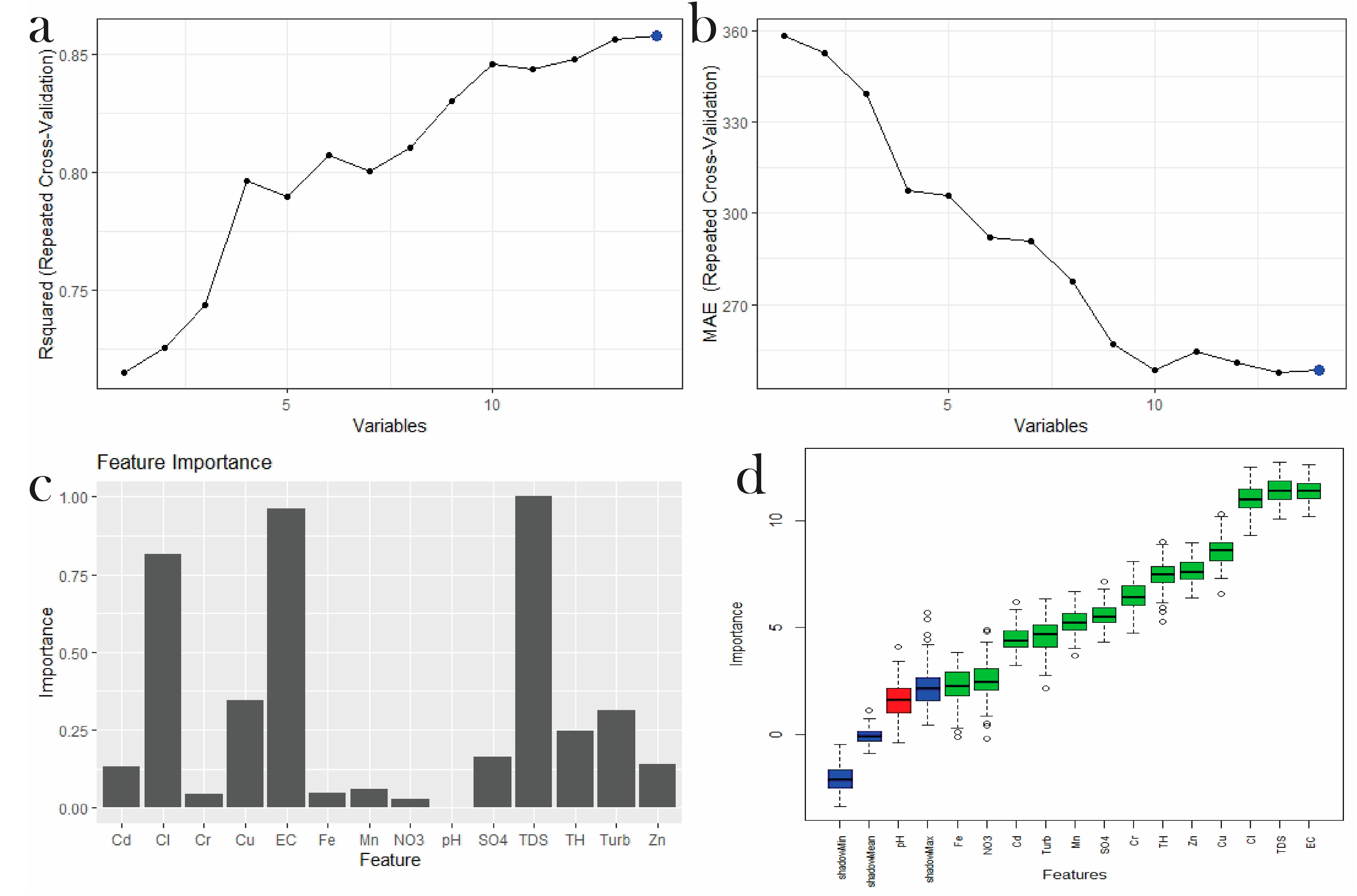
In the present study, we used RF-based REF with cross-validation, RF, and Boruta as feature selection before proceeding with modelling. The three advanced methods were trained and tested with higher accuracy. The result from the REF shows that an accuracy of over 0.86 can be achieved when fourteen variables are included in the modelling, while a smaller number of variables results in a lower accuracy (
Figure 3a,b). The kappa value also indicates that the inclusion of a larger number of parameters can reduce the probability of error (
Figure 3c). On the other hand, in the feature selection technique of RF and Boruta, pH is the redundant variable for WQI prediction and should therefore be excluded from the modelling (
Figure 3d). However, the advanced method REF provides some significance for pH, and since we theoretically assume that pH might have some significance for WQI, we decided to include it in the modelling.
3.3.2. Model Calibration under H2O Framework
In this study, four models, such as GBM, GLM, DNN, and the proposed stacking models were implemented under the H2O framework. The hyperparameters of GBM, GLM, and DNN models were tuned using the grid search technique. The calibration process involves testing various combinations of hyperparameters and selecting the combination that yields the lowest residual deviance. The hyperparameters of GBM model used for the grid search are the number of trees in the model (ntrees), the maximum depth of each tree (max_depth), the learning rate of the model (learn_rate), the fraction of rows to be used for each tree (sample_rate), the fraction of columns to be used for each tree (col_sample_rate), and the number of stopping rounds to prevent overfitting (stopping_rounds). Residual deviance is a measure of the difference between the observed and predicted response values. The lower the residual deviance, the better the model’s fit.
The ranges of the hyperparameters are as follows:
ntrees: 50, 100, 200, 500;
max_depth: 3, 5, 7, 9;
learn_rate: 0.01, 0.1, 0.3, 0.5, 0.7;
sample_rate: 0.5, 0.7, 0.9;
col_sample_rate: 0.5, 0.7, 0.9;
stopping_rounds: 5, 10, 15.
A grid search hyperparameter tuning is performed using the H2O GridSearch function. The function trains multiple models with different hyperparameter combinations, and the best performing model is selected. In this case, 81 models were generated and ranked by increasing residual deviance. The best performing model had a learn_rate of 0.2, max_depth of 6, ntrees of 29, and stopping_rounds of 0, with a residual deviance of 693,061.54.
The grid search hyperparameters for GLM are defined as alpha (regularization parameter), lambda (penalty parameter), and standardize (boolean variable indicating whether the data should be standardized before fitting the model). The range of alpha is 0.1, 0.5, and 0.7, lambda is 0.1, 0.5, 0.7, and standardize is [True, False].
The grid search hyper-tuning process is performed using the H2OGridSearch function, and the best combination of hyperparameters is selected based on the minimum residual deviance. In this case, 18 models were generated, and the best GLM model was selected from the grid search. The best combination of hyperparameters was alpha = 0.7, lambda = 0.1, and standardize = False, with a residual deviance of 14,902.67.
In this study, a grid search is performed on a DNN model with 729 possible combinations of hyperparameters. The hyperparameters include the number of hidden layers, number of neurons in each layer, activation function, dropout rate, learning rate, and regularization parameters. The ranges of different hyperparameters are as follows:
“hidden”: [32, 32], [64, 64], [128, 128] (number of neurons in each hidden layer);
“epochs”: 10, 20, 30 (number of passes through the training data);
“activation”: rectifier, tanh, maxout (type of activation function);
“input_dropout_ratio”: 0.1, 0.2, 0.3 (dropout rate for input layer);
“hidden_dropout_ratios”: [0.1, 0.1], [0.2, 0.2], [0.3, 0.3] (dropout rates for hidden layers);
“l1”: 1 × 10⁻⁵, 1 × 10⁻⁴, 1 × 10⁻³ (L1 regularization parameter);
“l2”: 1 × 10⁻⁵, 1 × 10⁻⁴, 1 × 10⁻³ (L2 regularization parameter);
“adaptive_rate”: True, False (learning rate adaptation);
“rho”: 0.9, 0.95, 0.99 (learning rate decay factor).
After training and evaluating all possible hyperparameter combinations using a fivefold cross-validation, the best model is selected based on the residual deviance metric, which measures the difference between predicted and actual values. In this case, the best model has the following hyperparameter values:
Activation function: Maxout;
Number of epochs: 30;
Number of neurons in each hidden layer: [64, 64];
L1 regularization parameter: 1 × 10⁻⁵;
L2 regularization parameter: 0.001;
Learning rate decay factor: 0.99.
This model achieved a residual deviance of 49,832.02, which is the lowest among all evaluated models.
3.3.3. Development of Stacking Model
The development of a stacking model involves combining multiple machine learning models to improve the predictive performance of the ensemble model. In the above example, the base models are three different models: best_gbm, best_glm, and best_dnn. These models are trained independently on the same dataset and generate their respective predictions.
The stacking ensemble model combines the predictions of these base models and uses them as input to a meta-learner model. The meta-learner model takes the base models’ predictions as input and generates the final prediction. In this example, the meta-learner algorithm is a deep learning algorithm, which is trained on the predictions of the base models.
During the training process, the stacking ensemble model uses cross-validation, which means that the model is trained on multiple subsets of the data, and the performance is averaged over all the subsets to avoid overfitting. The stacking ensemble model uses an automatic fold assignment scheme for the metal-earner and has no fold_column specified. In this way, the hybrid stacking model was developed.
3.3.4. CNN Model Calibration Using Bayesian Optimization
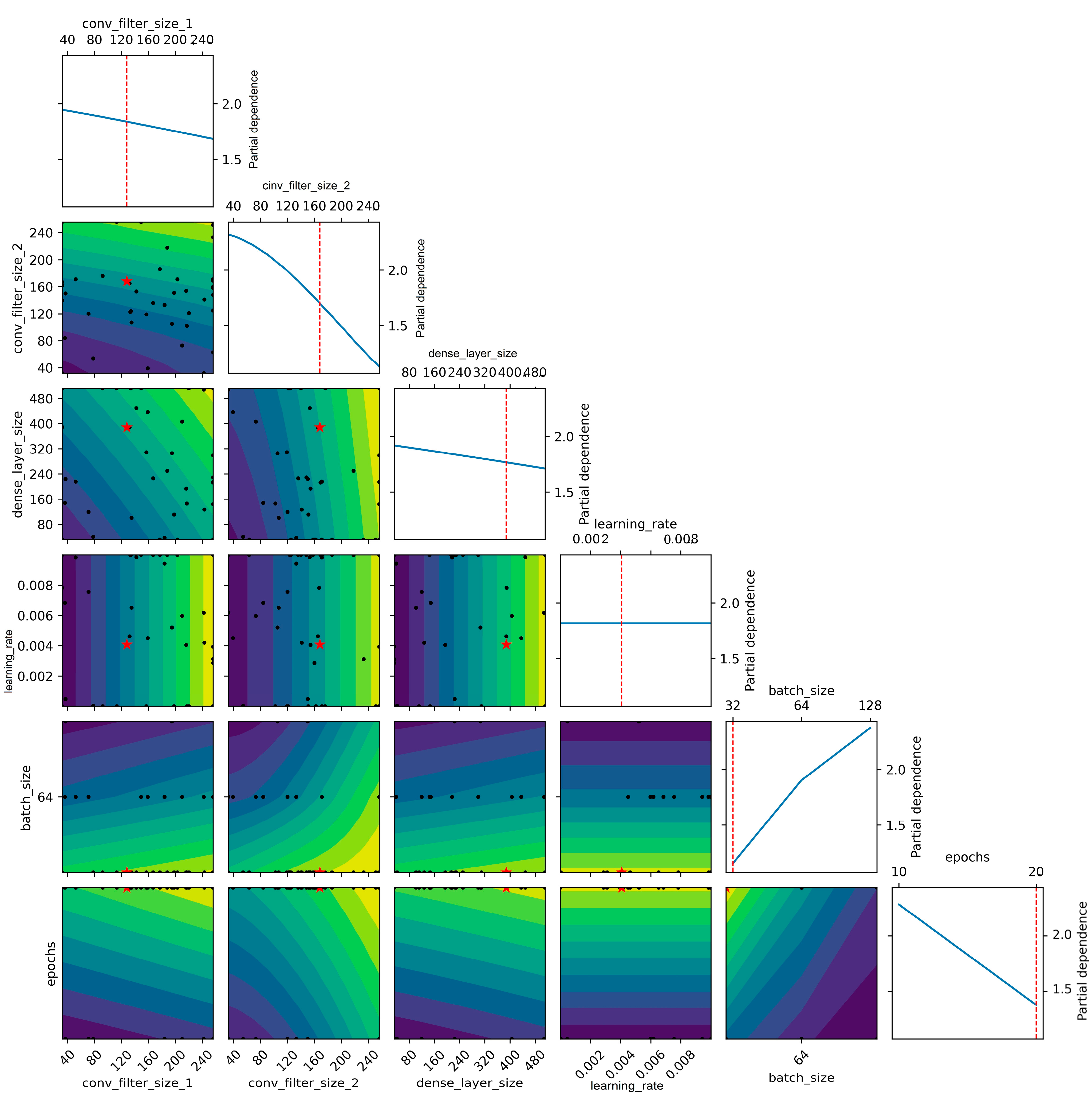
In this study, the Bayesian optimization algorithm is used for hyperparameter tuning, which involves defining a search space consisting of possible values for each hyperparameter. The search space for the current model includes six hyperparameters: conv_filter_size_1, conv_filter_size_2, dense_layer_size, learning_rate, batch_size, and epochs.
The range of the search space for each hyperparameter is defined using various objects from the skopt library. For example, Integer(32, 256, name = “conv_filter_size_1”) defines an integer hyperparameter named conv_filter_size_1 that can take values between 32 and 256. Similarly, Real(1 × 10⁻⁵, 1 × 10⁻², name = “learning_rate”) defines a real-valued hyperparameter named learning_rate that can take values between 1 × 10⁻⁵ and 1 × 10⁻².
The Bayesian optimization algorithm then uses these search spaces to sample different combinations of hyperparameters and evaluate the model’s performance using the evaluate_model function. After 50 iterations of sampling and evaluating, the algorithm identifies the best hyperparameters that minimize the validation loss.
To visualize the optimization process, the skopt library provides different plotting functions. The plot_objective function produces a 2D surface plot that shows the distribution of sampled points in the search space and the corresponding values of the objective function (in this case, the validation loss) (
Figure 4). The black points indicate the sampled points, and the red star indicates the best point found so far. At the end of each row of the 2D surface plot, there is a graph consisting of a blue line graph and a red vertical line. This graph shows the evolution of the objective function over the iterations of the Bayesian optimization algorithm, with the blue line representing the best value found so far and the red vertical line indicating the current iteration. The best hyperparameters identified by the algorithm are 256, 169, 153, 0.01, 32, 20, which correspond to the values for conv_filter_size_1, conv_filter_size_2, dense_layer_size, learning_rate, batch_size, and epochs, respectively. The validation loss obtained with these hyperparameters is 127,547.17.
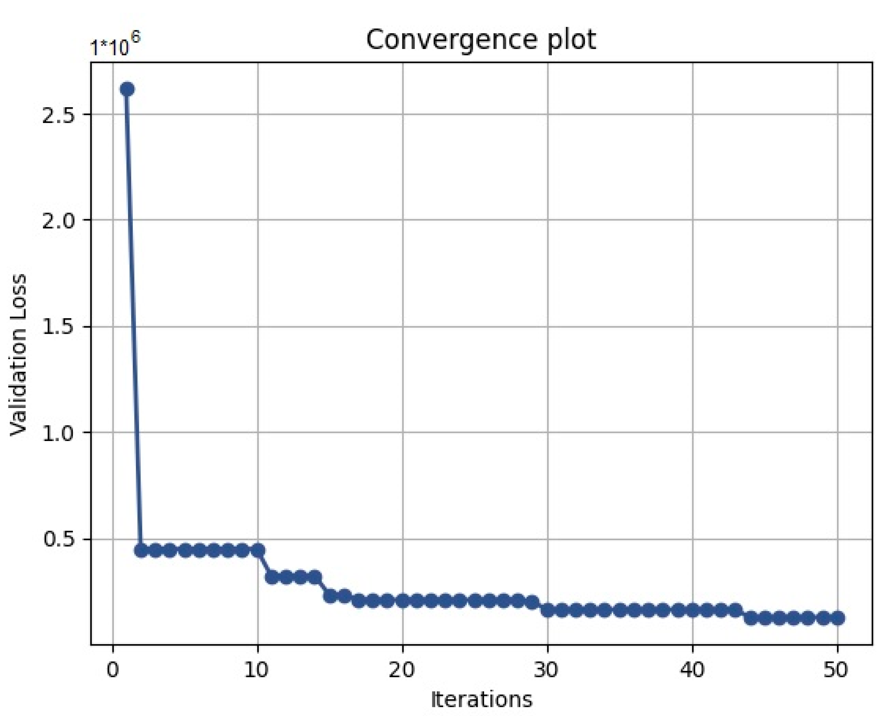
The plot_convergence function produces a convergence plot that shows the evolution of the validation loss over the iterations of the algorithm (
Figure 5). This plot confirms that the algorithm has converged after about 30 iterations, as the validation loss becomes flat. Overall, the Bayesian optimization algorithm allows for efficient and automated hyperparameter tuning that can help to improve the performance of machine learning models.
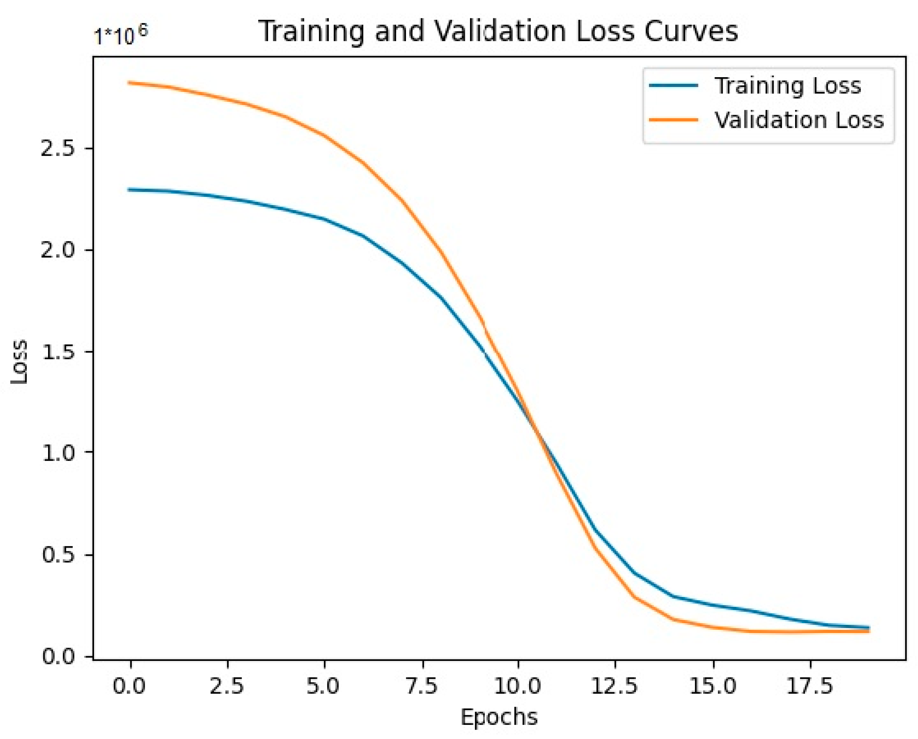
In this study, we plotted the learning curves of the final model, which is trained with the best hyperparameters on a given dataset (
Figure 6). The model is trained with a batch size of 32 and for 20 epochs. The training and validation loss and MAE values are initially high, indicating that the model is not performing well on the dataset. However, as the number of epochs increases, the training and validation loss and MAE values decrease gradually. This implies that the model is learning and improving its performance on the dataset with each epoch.
After 20 epochs, the training and validation loss and MAE values seem to be stabilized, indicating that the model has converged and is not improving much further with additional epochs.
3.4. Prediction and Validation of EWQI
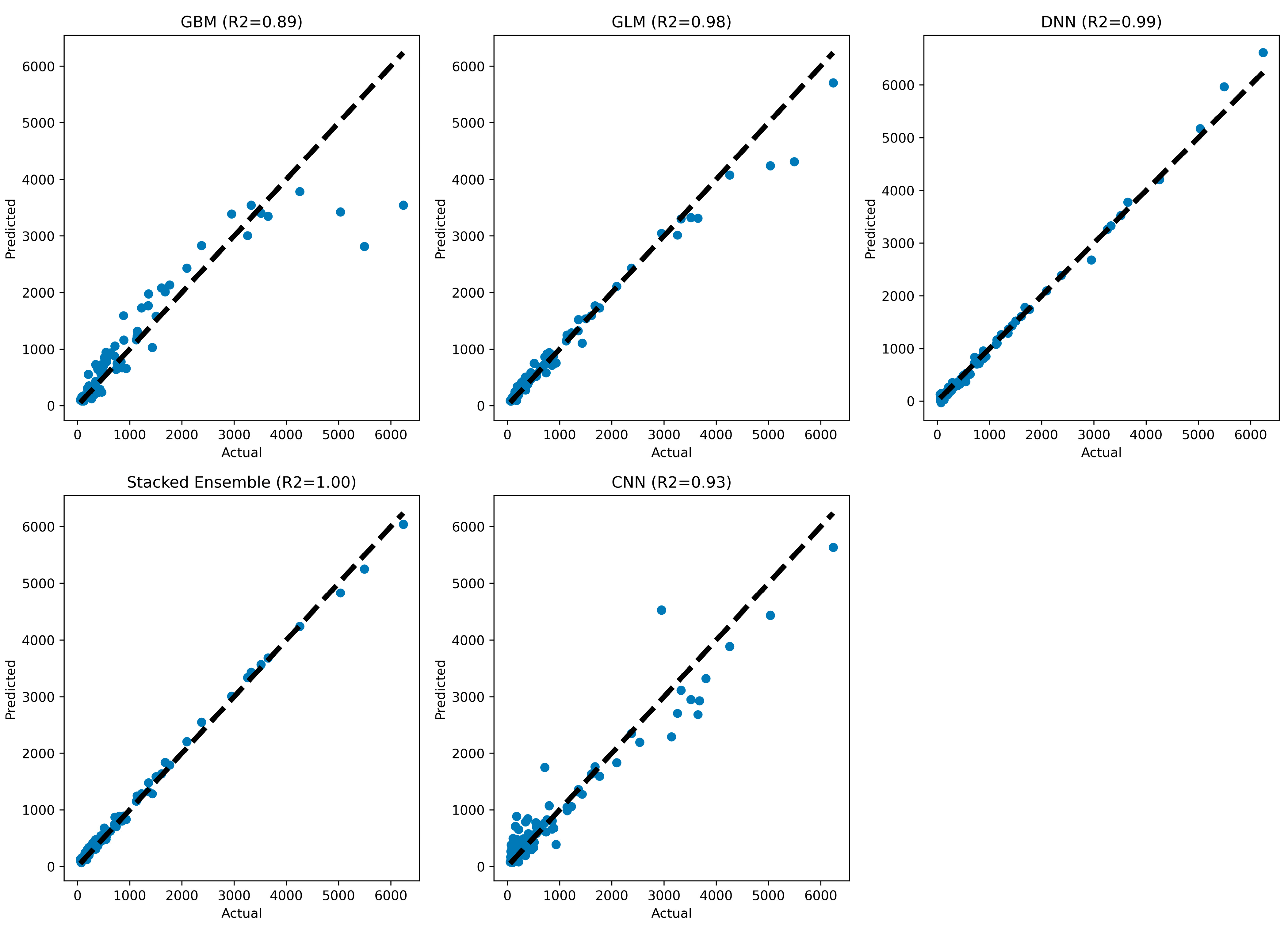
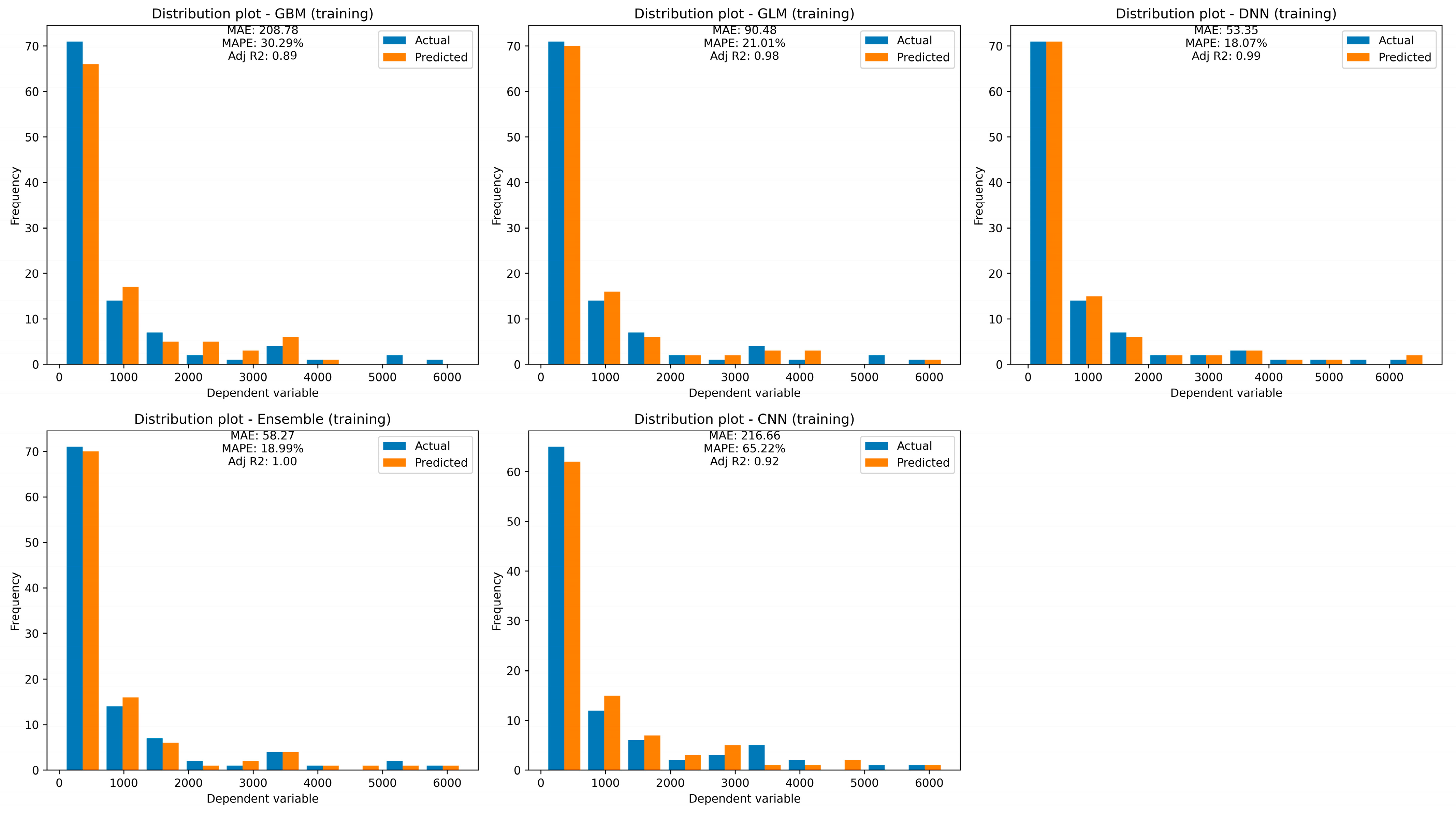
For training and testing datasets, WQI was predicted using GBM, GLM, DL, stacking (a mixture of the three models mentioned), and CNN models (
Figure 7 and
Figure 8).
The GBM model has an MSE of 209,945.56, an RMSE of 458.20, an MAE of 208.78, an RMSLE of 0.34, and an R2 value of 0.89. The GLM model has an R2 value of 0.98 on the training dataset, indicating that it explains 98% of the variability in the target variable. The DNN model has an MSE of 7292.23, an RMSE of 85.39, an MAE of 53.35, and an R2 value of 0.99. The stacking model has an MSE of 5840.50, an RMSE of 76.42, an MAE of 58.27, an RMSLE of 0.22, and an R2 value of 1, indicating that it explains all the variability in the target variable. The CNN model has a training RMSE of 336.10, a training MSE of 112,963.49, a training MAE of 216.66, and an R2 value of 0.93. To compare the performance of these models, we use the MSE, RMSE, MAE, and R2 values. Based on these performance statistics, the stacking model outperforms all other models, as it has the lowest values of MSE, RMSE, and MAE and the highest value of R2. Overall, the stacking model can be considered the best model based on the given information, followed by the DNN, CNN, GBM, and GLM models.
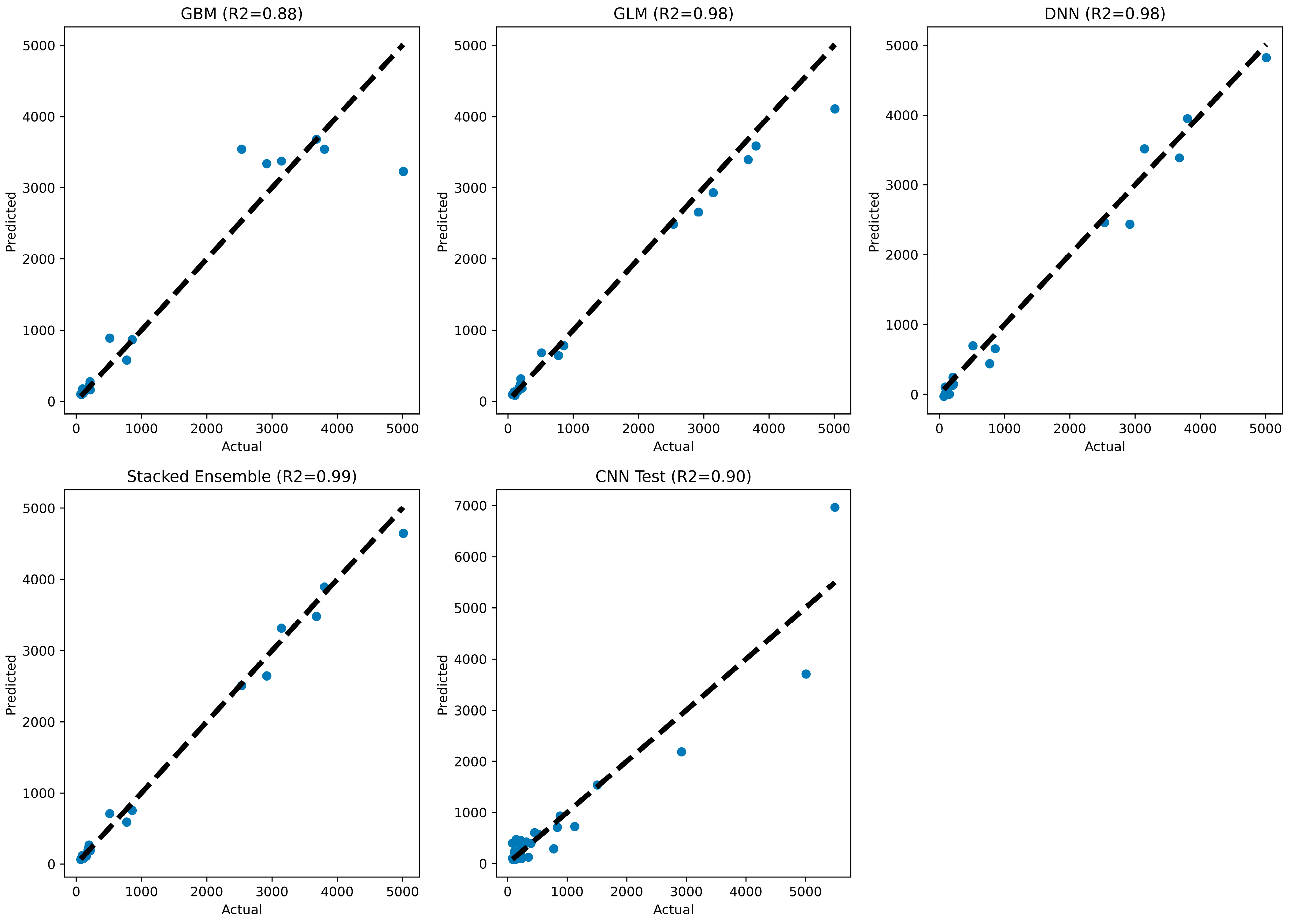
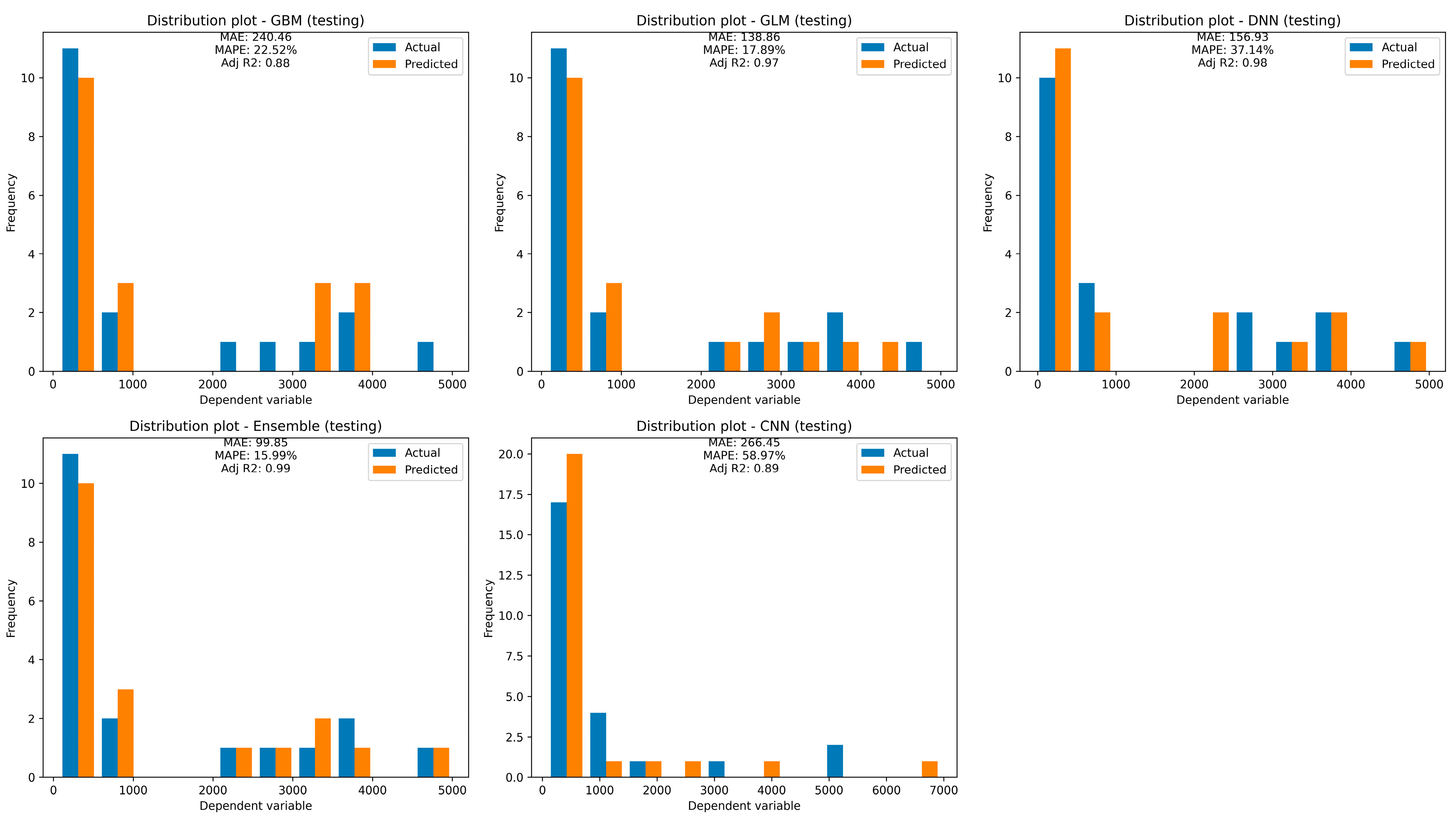
The given results are performance statistics for different all models on a testing dataset.
The GBM model has an MSE of 245,974.43, an RMSE of 495.96, an MAE of 240.46, an RMSLE of 0.27, and an R2 value of 0.88. The GLM model has a lower MSE of 59,453.28, an RMSE of 243.83, an MAE of 138.86, an RMSLE of 0.20, and a higher R2 value of 0.98. The DNN model has an even lower MSE of 40,535.88, an RMSE of 201.34, an MAE of 156.93, and an R2 value of 0.98. The stacking model has the lowest MSE of 19,894.03, an RMSE of 141.05, an MAE of 99.85, an RMSLE of 0.19, and a higher R2 value of 0.99. The CNN model has the highest RMSE of 456.90, an MSE of 208,754.47, an MAE of 266.45, and an R2 value of 0.90.
Based on the performance statistics, the stacking model appears to be the best-performing model, followed by the GLM model. The GBM and DNN models also performed reasonably well. Regarding the CNN model, it has a higher RMSE of 456.90 and an MSE of 208,754.47, which are much larger than those of the other models but still acceptable given the nature of CNN models, especially with fewer data. However, its R2 value of 0.90 is still reasonable, indicating that the model can explain 90% of the variance in the target variable.
However, based on the given evaluation metrics, the stacking model is the best model for this regression problem, followed by the GLM model, DNN model, GBM model, and CNN model.
3.5. Comparison of the Models
In this study, five different models (GBM, GLM, DNN, stacking, and CNN) were evaluated for their ability to predict WQI using training and testing datasets. The performance of each model was assessed based on MAE, MAPE, adjusted R
2, and residual distribution plot. The GBM model had a MAPE of 30.29% and an adjusted R
2 of 0.89, while the GLM model had a MAPE of 21.01% and an adjusted R
2 of 0.98. The DNN model had a MAPE of 18.07% and an R
2 of 0.99, and the stacking model had a MAPE of 18.99% and an adjusted R
2 of 1. The CNN model had a higher MAPE of 65.22% and an adjusted R
2 of 0.92 (
Figure 9).
When evaluating the models using the testing data, the GBM model had a MAPE of 22.52% and an adjusted R
2 of 0.88, while the GLM model had a MAPE of 17.89% and an adjusted R
2 of 0.89. The DNN model had a MAPE of 37.14% and an R
2 of 0.98, and the stacking model had a MAPE of 15.99% and an adjusted R
2 of 0.99. The CNN model had a higher MAPE of 58.77% and an adjusted R
2 of 0.89 (
Figure 10).
The t-statistic and p-value were also calculated for each model on both the training and testing data. The results showed that the GLM and stacking models had the most significant t-statistic values on the training data, indicating that their performance was significantly better than random chance. However, on the testing data, the GLM, DNN, and stacking models had significant t-statistic values, indicating that their performance was significantly better than random chance. Based on the overall performance metrics, it can be concluded that the GLM, stacking, and DNN models are the best models for predicting WQI, with the stacking model being the best performer overall. The CNN model had the poorest performance, indicating that it may not be the best model to use for management strategies.
3.6. Improvement in Decision-Making by Coupling ML and DL Models with XAI
The combination of ML and DL models provides a robust and accurate way to make predictions with computing variables importance to the prediction, while XAI provides transparency and interpretability, making it easier for the decision-makers to understand the relationships between inputs and outputs. In this combination, ML models provide a simple and interpretable approach to decision-making, while DL models provide high accuracy and the ability to model complex relationships. By coupling these models with XAI, the decision-makers can benefit from both the accuracy of DL models and the interpretability of ML models. XAI can provide a clear explanation of the decision-making process and help the decision-makers to understand the relationships between inputs and outputs, making it easier to make informed decisions.
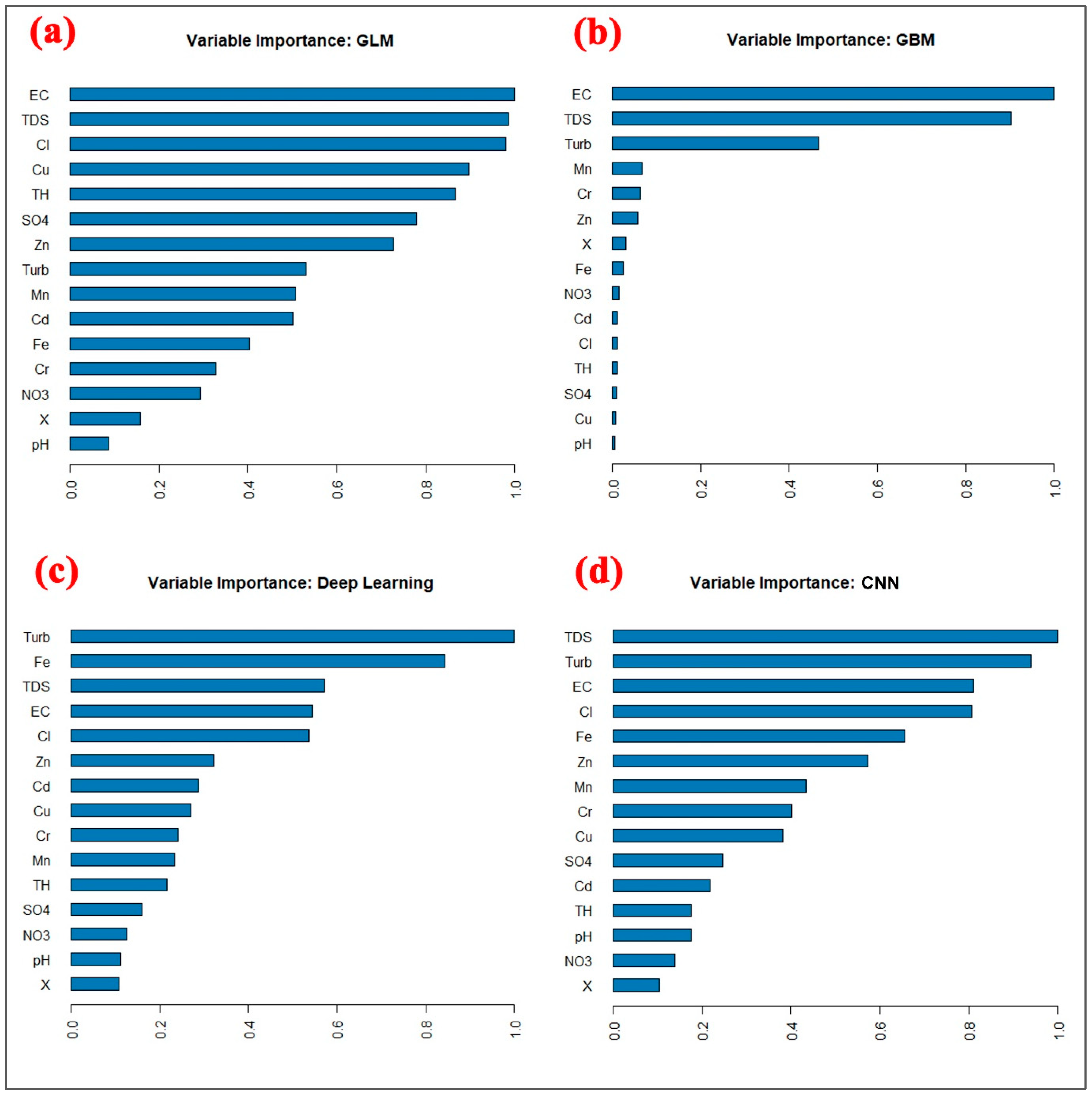
3.6.1. Computation of Variable Importance Using ML and DL Models
In this research, the variable importance was computed during predicting the WQI using the ML and DL models (
Figure 11). Variable importance provides a measure of the significance of each input feature in the prediction of WQI, allowing the decision-makers to understand which factors have the greatest impact on water quality. By understanding which factors have the greatest impact on water quality, the decision-makers can prioritize actions to improve water quality and make informed decisions about resource allocation. Furthermore, the significance of all parameters was computed using GLM (
Figure 11a). It demonstrates that electrical conductivity (EC) is most important, followed by total dissolved content (TDS), chloride (Cl), and Cu, while pH, nitrate (NO
3), and Cr are the least important.
Figure 11b shows the weighting of all input parameters generated by the GBM model. It was discovered that EC is the most important parameters followed by TDS and turbidity, while pH, Cu, and SO
4 have the least relevance. The weights for all parameters were determined using DL based on this model structure and are presented in
Figure 11c. It demonstrates that turbidity, iron (Fe), and TDS have the most important parameters, while pH, NO
3, and SO
4 are the least important parameters. We calculated the importance of the variables for CNN architecture (
Figure 11d). The optimised CNN architecture calculated the highest importance for TDS in WQI prediction, followed by turbidity (0.95), EC, and Cl. On the other hand, the simple CNN architecture shows that TDS, turbidity, and EC have the highest importance, while NO
3, pH, and total hardness (TH) have lower importance. Therefore, the decision-makers should carefully monitor highly significant parameters related to water quality in the study area and develop management plans that prioritize these influential factors.
3.6.2. Deep Insights of the Black-Box Model for Obtaining More Information
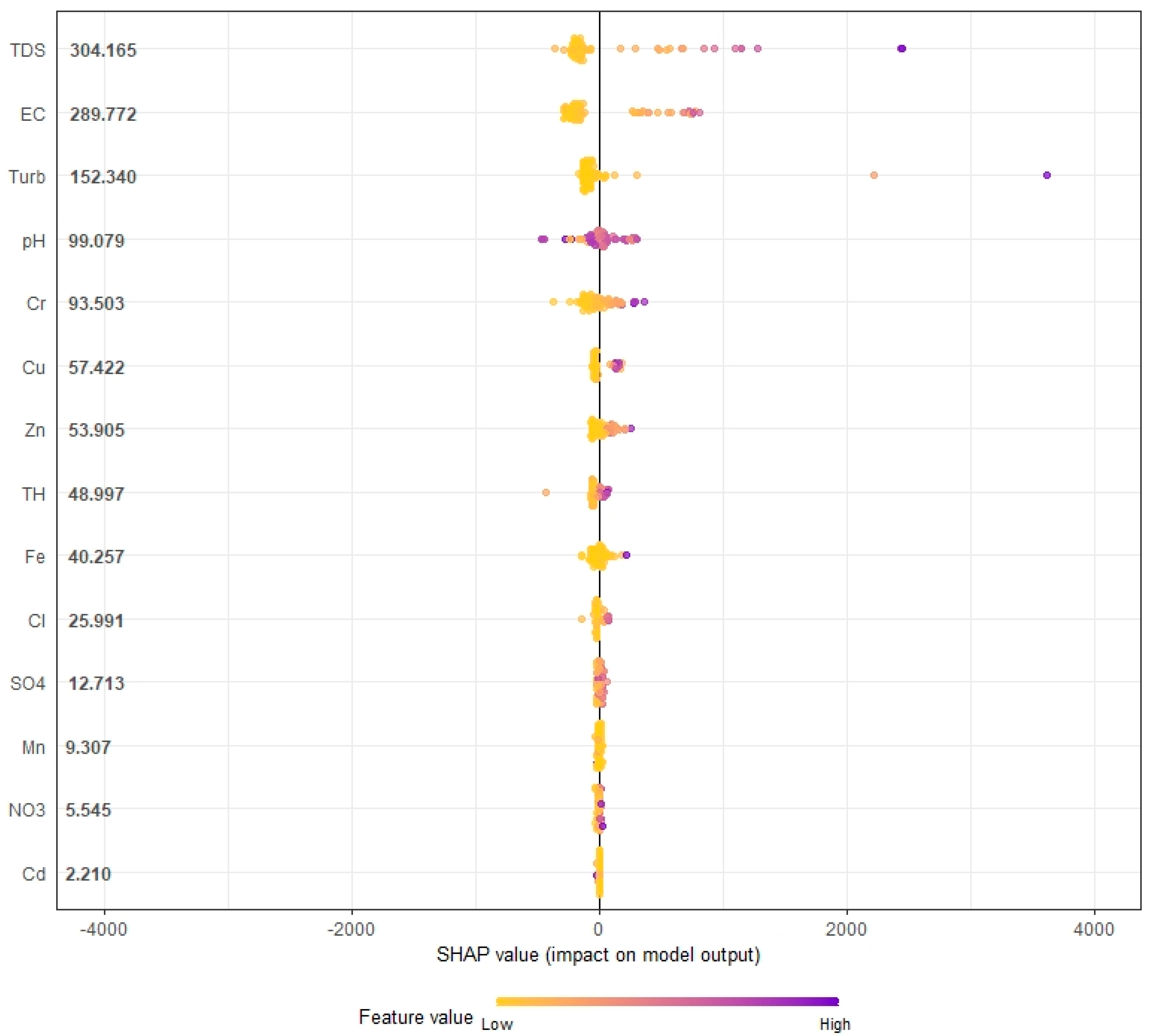
In the present study, we computed the SHAP value using a XGBoost model to acquire more information from WQI prediction to improve the decision-making for water quality management (
Figure 12). XGBoost-based SHAP summary plots can provide valuable insights for decision-making in water quality management. The SHAP summary plot is a graphical representation of the contribution of each input feature to the prediction of WQI. The SHAP summary plot shows the mean contribution of each input feature to the prediction, as well as the range of possible contributions for each feature. This provides a clear and interpretable way to understand the relationships between inputs and outputs and helps to identify which factors have the greatest impact on water quality. In water quality management, the SHAP summary plot can be used to prioritize actions to improve water quality. By understanding which factors have the greatest impact on water quality, the decision-makers can target their efforts where they will have the greatest impact. In the present study, it can be seen that high values of TDS, EC, turbidity, pH, Cr, CU, and Fe have the highest impact on the poor water quality (
Figure 12). Therefore, the management policy should consider these parameters for maintaining the standard water quality.
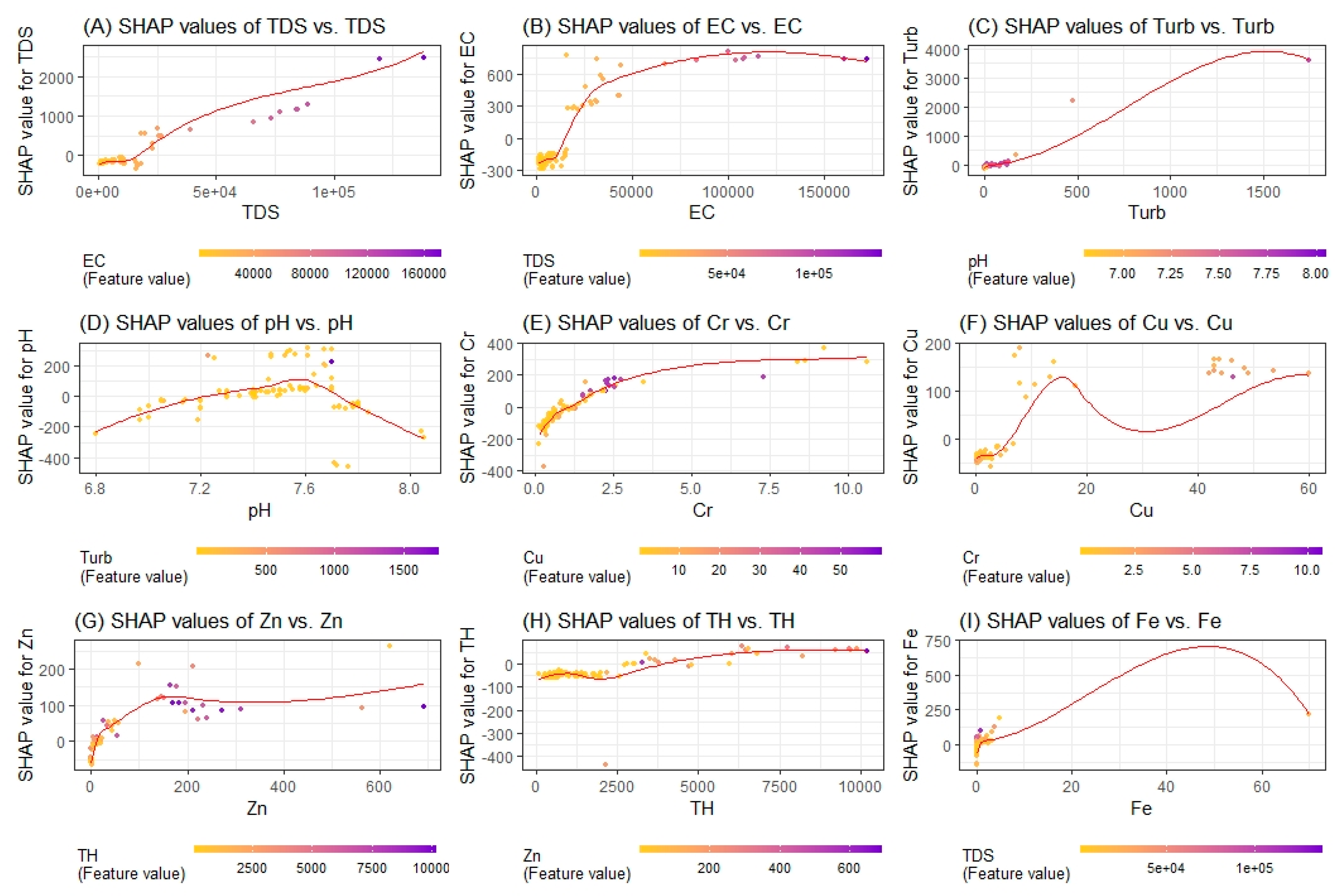
In the present study, to gain more information, we computed an interaction plot through the XGBoost-based SHAP value (
Figure 13). The XGBoost-based SHAP interaction plots provide valuable insights for decision-making in water quality management. They show how changes in one input feature can affect the prediction of WQI, as well as how this relationship is affected by changes in another input feature. Therefore, the SHAP interaction plot provides a clear and interpretable way to understand the relationships between inputs and the prediction of WQI, helping the decision-makers to prioritize actions to improve water quality, understand trade-offs, and make informed decisions about resource allocation. As indicated by the SHAP interaction plot, the very high values of total dissolved solids (TDS) and electrical conductivity (EC) are the main drivers of poor water quality. These parameters show a nonlinear relationship with the water quality index (WQI), meaning that even small increases in their levels can have a significant impact on water quality.
Based on these findings, the policy for water quality management should prioritize reducing TDS and EC levels in the water. This can be achieved through various measures, such as better wastewater treatment and tighter regulations on industrial and agricultural practices that contribute to these pollutants. Additionally, pH, turbidity, Fe, and TH also have nonlinear relationships with WQI, and after exceeding certain limits, they can cause very high pollution. The policy should also consider monitoring and controlling these parameters to maintain water quality. In conclusion, the policy for water quality management should prioritize reducing TDS and EC levels and also monitor and control pH, turbidity, Fe, and TH levels. This will help to ensure that water quality remains high and within acceptable levels.
4. Discussion
As the global population increases, the demand of fresh water for the domestic and other purposes also increases. However, the demand and supply of water are not always identical due to uneven distribution of water resources, and some regions have surplus of water, while some are facing the scarcity of fresh water [
2,
69,
70,
71]. Furthermore, the contamination and pollution of water resources also increasing as a consequence of the anthropogenic activities and improper sanitation [
72]. Thus, it is the need of time to examine the quality of fresh water for the water resource management and ensuring long-term water balance [
73,
74]. For this, researchers have tried to examine and predict the water quality in different parts of the world using different techniques [
6,
19,
25,
27,
48]. In this study, the prediction of WQI by proposing a new stacking framework along with the GLM, DBM, DNN, and CNN models in the Al Qunfudhah region which is located on the Red Sea coast of Saudi Arabia. As the region has a semi-arid climate, it is facing scarcity of fresh water. Moreover, the contamination and pollution of water is also very common in this region due to the heavy metal contamination as well as sea water intrusion [
75].
In this study, a stacking model of GLM, GBM, and DL model was applied along with CNN for the prediction of WQI using fifteen water quality parameters. Although, several approaches and techniques have been applied for predicting the WQI, all these techniques have certain shortcomings. The traditional statistical methods although produces good results, they are time consuming and are complicated [
76,
77]. Therefore, researchers have developed and applied advanced techniques based on artificial intelligence (AI) for the analysis and prediction of WQI [
25,
26,
33]. The main advantage of AI-based techniques is they produces the reliable outcomes in very short time even with the fewer data [
33]. In this study, although all the AI-based DL and ML models produced reliable results, the stacking model (RMSE < 2.4) and CNN (RMSE < 1.6) performed better than the other models.
The AI-based ML models have been applied in a number of hydrogeological studies such as for surface and subsurface water quality monitoring [
76], flood and landslide hazard mapping [
78], groundwater potential zoning [
63,
79], etc. However, the DL models such as CNN and DNN were used only in a few studies [
25,
80]. Based on the findings of previous studies, it was reported that the DL models had produced better outcomes in the time-series analysis of hydrometeorological data than the traditional ML and ensemble ML models [
81,
82,
83]. In this study, the stacking model showed the highest correlation coefficient (98% in both training and testing phase) between actual and projected WQI followed by CNN (96% in training and 90% in testing). This indicates that the stacking and GLM and DNN models have better accuracy in predicting the WQI than other models. Although the CNN model showed a relatively high R2 value, other statistical measures indicate that it is actually the worst-performing model out of the five tested. This may be due to the fact that there were fewer input data available for training the model. While we attempted to improve its performance through Bayesian optimization, the results did not meet our expectations. Further, among all the parameters, the turbidity (0.143) showed the highest weightage in WQI prediction while pH (0.004) showed the minimum weightage. Further, the significance of the parameters was examined using the aforesaid model which showed that the EC, Fe, and TDS were the most important parameters in WQI prediction in Al Qunfudhah region. In recent years, the region has witnessed significant increase in petrochemical and heavy industries [
84] which may have increased the contamination of EC and Fe in the water [
85,
86].
A DNN-based uncertainty analysis was performed in this research to examine the significance and uncertainty of the WQI parameters for the output used in this study which showed the importance of each parameter for the WQI prediction. The uncertainty analysis is an important aspect of WQI prediction which may affect the planning and policy making [
32,
87]. Although, the stacking model had the highest accuracy in the prediction of WQI in this research, it is to be noted that the stacking model was created using the two deep learning models as base learners. Thus, it is possible that the performance of deep learning may be further increased by combining it with the other models such as ML models and traditional statistical models. Moreover, Afzaal et al. [
88] noted that the performance of DL models may be increased by increasing the number of input parameters. This is identical to the findings of this research that CNN model requires large dataset to achieve good performance in WQI prediction. Thus, in the future studies, authors may use the stacking models as well as combined the DL models for the WQI prediction as well as other kinds of hydrological and meteorological studies.
The condition indicated by the XAI with very high values of total dissolved solids (TDS), zinc, and electrical conductivity (EC), which have a strong impact on water quality, is a serious problem for water management. These parameters have a nonlinear relationship with the water quality index (WQI), which means that even small increases in their values can lead to significant deterioration of water quality. The finding that pH, turbidity, Fe, and TH also have a nonlinear relationship with the WQI, but only cause very high pollution when certain limits are exceeded, underlines the importance of monitoring and controlling these parameters as well. This situation raises a number of important questions for water management, such as the following:
- (1)
What are the sources of TDS, zinc, and EC pollution, and how can they be reduced or eliminated?
- (2)
What measures can be taken to monitor and control pH, turbidity, Fe, and TH in the water to ensure that they do not lead to very high levels of pollution?
- (3)
What are the trades-offs between reducing TDS, zinc, and EC levels and the other parameters such as pH, turbidity, Fe, and TH? For example, reducing TDS levels can lead to increased pH, which can have a negative impact on water quality.
- (4)
What influence does the nonlinear relationship between TDS, zinc, EC, and WQI have on decision-making in water management?
- (5)
What is the role of stakeholders such as industry, agriculture, and government in improving water quality and reducing pollution levels?
These questions highlight the need for a comprehensive and integrated approach to water management that takes into account the interactions between different parameters and their relationships to water quality. Addressing this situation requires concerted action by all stakeholders, including industry, agriculture, government, and the wider public, to ensure that water quality remains high and within acceptable limits. This may enhance the quality of outcomes and will be beneficial for the effective management and conservation planning, especially in the water-scarce regions such as Saudi Arabia and other arid and semi-arid countries.
5. Conclusions
In the present research, a new stacking framework based on GLM, DBM, and DNN models was developed for the WQI prediction along with the CNN model in the Al Qunfudhah region of Saudi Arabia. The XGBoost-based SHAP was used as a XAI technique for extracting useful information to improve the decision-making. This study shows that the stacking model has a better performance in WQI prediction followed by GLM, DNN, GBM, and CNN. The aforesaid framework indicates that EC, Fe, and TDS have the highest significance in WQI prediction. Hence, these parameters must be monitored in order to control and reduce water pollution. This study shows that the correlation coefficient between actual and projected WQI indicates that the stacking model has the highest correlation at both training and testing phase (0.98), while the CNN model stood second with a correlation coefficient of 0.96 at the training phase and 0.90 at the testing phase. This means that stacking and CNN models have the best accuracy in WQI prediction compared with the other models. The SHAP interaction plot provides valuable insights into the drivers of water quality and their relationships with the WQI. The high values of TDS, zinc, and EC indicate poor water quality, and their nonlinear relationship with WQI highlights the need for immediate action to reduce these pollutants. Additionally, monitoring and controlling other parameters such as pH, turbidity, Fe, and TH are also important, as they can cause very high pollution after exceeding certain limits. It is crucial for the decision-makers to take these findings into consideration and implement a comprehensive and integrated approach to water management, involving all stakeholders, to reduce pollution levels and maintain high water quality for the benefit of communities and the environment. Future studies on the monitoring of surface and subsurface water quality may use this study as a springboard. Future studies should examine whether it is possible to successfully use ML and DL models in other parts of the world. Moreover, the future research may be focused on improving the DL-based sensitivity analysis, potentially through the use of different feature extraction techniques. Because ML and DL models are useful tools for examining highly nonlinear interactions, the indirect effects of WQI on the surface water communities such as fish, phytoplankton, and zooplankton, may be interesting to study in future research.


