Spatial or Random Cross-Validation? The Effect of Resampling Methods in Predicting Groundwater Salinity with Machine Learning in Mediterranean Region

Abstract

Machine learning (ML) algorithms are extensively used with outstanding prediction accuracy. However, in some cases, their overfitting capabilities, along with inadvertent biases, might produce overly optimistic results. Spatial data are a special kind of data that could introduce biases to ML due to their intrinsic spatial autocorrelation. To address this issue, a special resampling method has emerged called spatial cross-validation (SCV). The purpose of this study was to evaluate the performance of SCV compared with conventional random cross-validation (CCV) used in most ML studies. Multiple ML models were created with CCV and SCV to predict groundwater electrical conductivity (EC) with data (A) from Rhodope, Greece, in the summer of 2020; (B) from the same area but at a different time (summer 2019); and (C) from a new area (the Salento peninsula, Italy). The results showed that the SCV provides ML models with superior generalization capabilities and, hence, better prediction results in new unknown data. The SCV seems to be able to capture the spatial patterns in the data while also reducing the over-optimism bias that is often associated with CCV methods. Based on the results, SCV could be applied with ML in studies that use spatial data.

1. Introduction

The abundance of available data, as well as new and innovative techniques like machine learning (ML) methods, are increasingly used in the environmental sciences [1,2,3,4,5]. Due to their expanded capabilities (increased accuracy, efficiency, model fitting simplicity, etc.), ML approaches provide several advantages in modeling phenomena without the constraints or downsides of regression methods [6,7,8].

Machine learning models that are robust and efficient at making realistic predictions typically assume that the data used to train them is independent and identically distributed (i.i.d.) [7,9,10,11,12]. However, when this assumption is violated, it can lead to overfitting the highly flexible methods to the training data and underestimating spatial prediction errors [13]. This can result in over-optimistic validation statistics estimates [7] and a biased assessment of the model’s capability to generalize to independent data [14], leading to models with poor prediction accuracy.

Spatial autocorrelation that intrinsically characterizes spatial data poses a significant challenge when assessing the performance of machine learning (ML) models. Traditional resampling methods like conventional random cross-validation (CCV), which assume independent and identically distributed (i.i.d.) data, tend to produce over-optimistic results when applied to spatial data [11,12,15]. To overcome this issue, various techniques called spatial cross-validation (SCV) have been proposed [12,13,16,17]. These methods divide the data into spatially non-overlapping subsets, such as blocks or buffers, which are then used for cross-validation.

However, whether SCV is effective and to what extent is not straightforward and depends on multiple factors such as the prediction area (interpolation-extrapolation), the spatial autocorrelation of the landscape (long-sort autocorrelation ranges of predictors), the sampling pattern (regular-clustered distributed training samples) and the geographical prediction space (distances from prediction locations to its nearest training samples) [18]. Apart from that, one common challenge of these SCV techniques in determining the appropriate size of blocks or buffers in SCV. The size must be large enough to avoid data autocorrelation but not so large that the testing dataset is significantly different from the training dataset, leading to an accidental extrapolation [12]. One of the proposed methods, that is also applied in the current study, is the use of the auxiliary variables’ existing autocorrelation as a rough indicator of the block size [19].

Groundwater salinity is a significant problem that has an impact on the quality and productivity of agricultural areas [20,21]. Salinity is caused by accumulated dissolved salts in the soil, which can be generated by various sources, including irrigation, natural processes, and groundwater [22,23,24]. Groundwater salinity is particularly relevant in arid and semi-arid regions where the water table is shallow, and the water is highly saline due to limited recharge and high rates of evapotranspiration [25].

The timely identification of seawater intrusion is crucial to apply proper mitigation measures and strategies. To this aim, several methods have been proposed that include, i.e., the use of classic hydrogeochemical approaches and environmental isotopes [26], hydrogeochemical modeling and data analysis [27], and joint application of geochemical and geophysical methods [28,29].

Electrical conductivity (EC), a measure of the water’s ability to conduct an electrical current, is one of the most commonly adopted indicators of groundwater salinity [30]. The water becomes more saline as EC increases. Crop yields may be affected by high EC levels, as well as crop quality and plant disease risk [25].

The salinity of groundwater should be measured for various reasons. First, it reduces field productivity and can reduce crop yields and quality, resulting in economic losses for farmers [21,25]. In addition, since sources of drinking water are contaminated by groundwater with excessive salt concentrations, this can have an impact on human health [31,32]. Lastly, groundwater salinity can affect the chemical and structural composition of the soil, resulting in long-term degradation of the soil [33,34].

To mitigate the effects of groundwater salinity, it is essential to monitor the water’s electrical conductivity (EC) and understand its sources. The dominant factor that causes increased EC values is salinization, mostly related (but not limited) to seawater intrusion. However, additional sources or processes could also lead to elevated values, such as pollution by nitrates or heavy metals, natural weathering of geological formations, excessive use of fertilizers, urbanization, improper waste management, etc.

Therefore, the EC measurements may provide useful and significant information to develop management strategies that reduce the impact of salinity on agriculture and the environment [34], depending on its cause. These techniques can include developing irrigation practices, selecting salt-tolerant crops, and implementing measures to avoid salt leakage into groundwater [35], as well as preventing pollution, sustainable fertilization practices, and rational waste management.

In the present paper, the performance of conventional random cross-validation (CCV) and spatial cross-validation (SCV) methods is evaluated in the context of groundwater salinity estimation by electrical conductivity in the Mediterranean region. Three data sets were used in this study: A) from the area of the Rhodope pilot site in Greece in the summer of 2020, B) from the same area in Greece but with data collected in the summer of 2019 and C) from the Salento peninsula in southern Italy in 2020. In this way, we were able to evaluate the predictive capabilities of the ML models built using CCV and SCV in different cases: (A) in the same data set, (B) in a data set from a different time, and (C) in a data set from a different location. Specifically, the first dataset (A) was randomly split into training (A^train: 80% of A) for creating the ML models and testing (A^test: 20% of A) for assessing the models’ performance. The training dataset (A^train) was subsequently split with either CCV or SCV, and different ML models were trained using Quintile Random Forest (QRF), Random Forest (RF), and Gradient Boosting Machines (GBM) algorithms. The best ML model for each algorithm was used to make predictions on the A^test, B, and C datasets, and the results were compared to evaluate the effectiveness of the different cross-validation methods.

2. Materials and Methods

2.1. Area of Study and Water Sampling

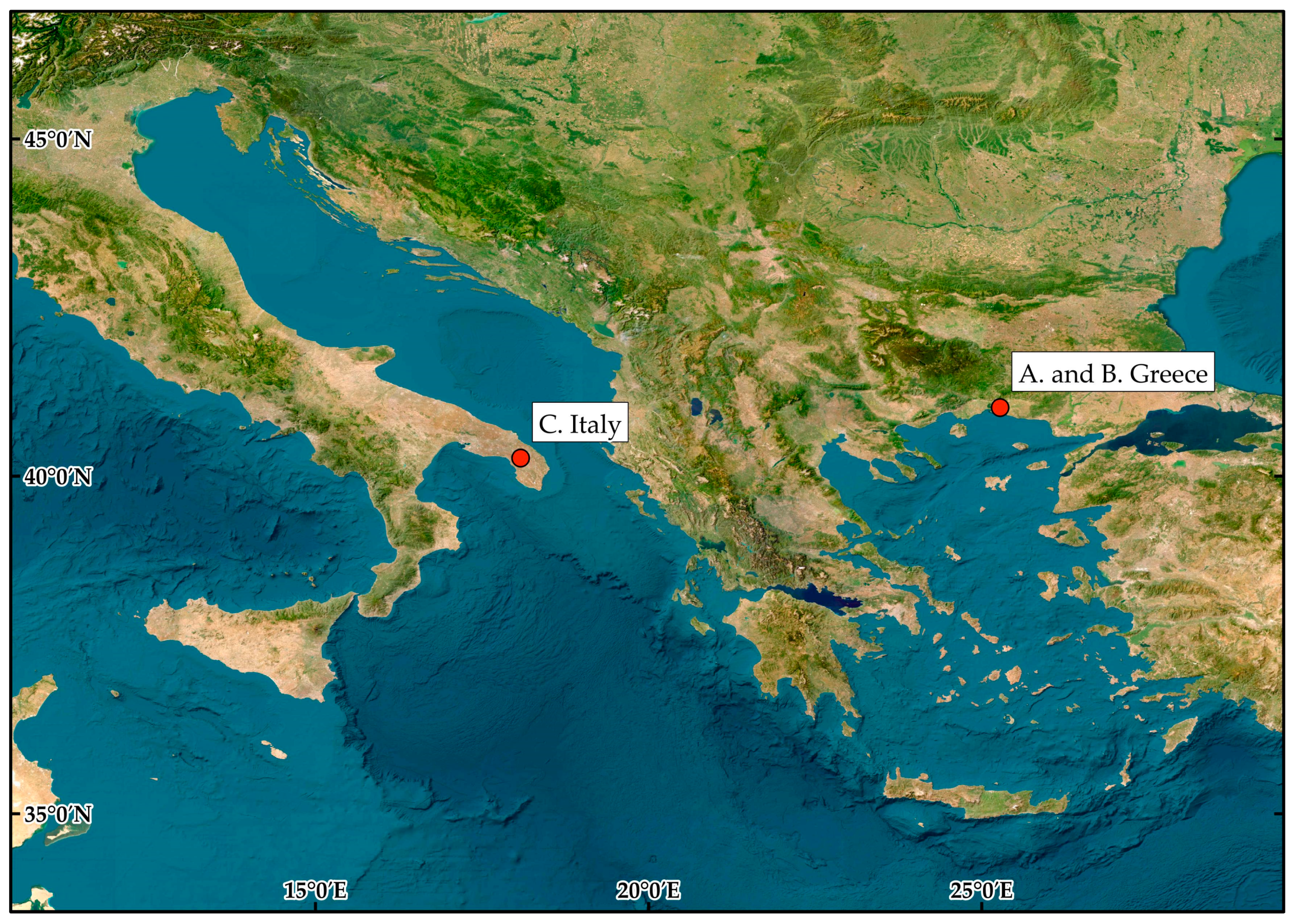
In the current study, three datasets were collected from two areas in the Mediterranean region with similar salinization problems (Figure 1). These datasets were collected as part of the MEDSAL Project [36], which aims to ensure the availability and quality of groundwater reserves along the Mediterranean coast.

The first area, the Rhodope pilot site (RHO), is in northeastern Greece and covers an area of 165.1 km². Most of the land is used for agriculture, and the permanent population is mainly employed in agricultural activities and tourism. The climate is warm-summer Mediterranean, and the area is mostly semi-hilly with a few scattered flat areas. Some lowlands have been formed by the combined action of the local hydrographic network. The area also includes several ephemeral streams, ditches, open water sources, and two surface reservoirs (Vistonida and Ismarida Lakes). The geological framework of the RHO pilot site consists of a Paleozoic metamorphic substrate (the Rhodope massif) overlain by more recent post-alpine formations of the Pliocene, Pleistocene, and Quaternary age. The more recent formations are of the Holocene age and consist of non-consolidated deposits of alluvial origin and different granulometric compositions. These formations are important for recharging the area due to their high permeability.

Concerning hydrogeology, two main aquifers are identified: a shallow semi-confined aquifer with an average thickness of 35 m and of limited hydrogeological potential and an underlain thicker one (50–100 m), which is confined and hosts the regional groundwater reserves. Irrigation schemes applied in recent decades due to intense agricultural activities led to a significant drawdown of groundwater, which sometimes reaches 30 m or even more. This has caused saline water to encroach on the coastal parts of the area. Lake Vistonida appears to be the main intrusion front, as well as the lagoons located at the southern boundary of the area. The potentiometric surface map of the aquifer system revealed that the hydraulic head is greatly reduced due to the overexploitation of groundwater, clearly demonstrated by the permanent regional cone of depression formed in the potentiometric surface of the aquifer system.

The second area is the Salento (SAL) coastal aquifer that is in the Salento Peninsula, Southern Italy, and is bordered by the Adriatic Sea, the Ionian Sea, and the Murgia territory. The climate is of Mediterranean type, with mild winters and hot summers. The area is highly urbanized, and agricultural land occupies 82.81% of the total area. The total annual precipitation shows a 2.4 mm/decade decrease, with an increase in drought periods between 1980 and 2011. The aquifer coincides with the limestone formation of the Upper Cretaceous–Palaeocene, belonging to the Mesozoic carbonate platform. It consists of layers and banks of variously fractured and karstified limestone and constitutes the geological basement of the SAL territory. Recharge mechanisms are complex, conditioned by the multifaceted permeability structure formed by epikarst, low permeability unsaturated zone, karst surface and subsurface features, fracture zones, and main discontinuities. The SAL aquifer is in coastal condition, with fresh groundwater floating as a lens on intruding seawater and saltwater of marine origin. Groundwater salinization mainly derives from saltwater upcoming because of exploitation. Environmental concerns include climate change, uncontrolled exploitation by private wells, excess phytosanitary treatments in agriculture, potentially contaminated sites, incomplete water depuration plants, and soil desertification.

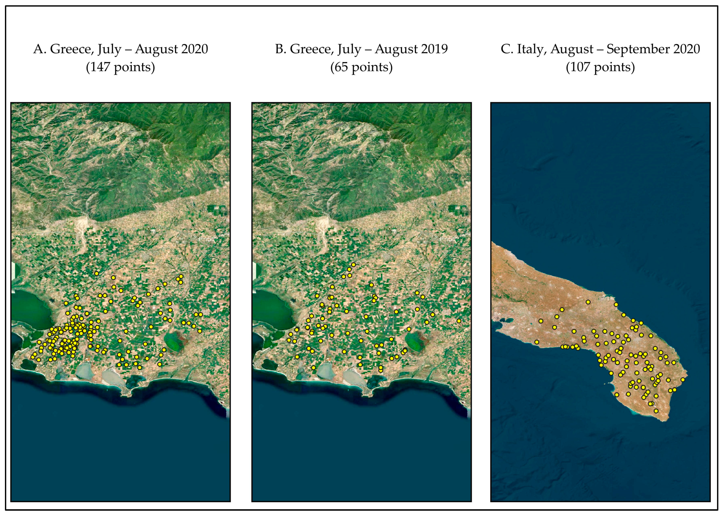
Three distinct datasets were created from the two study areas (Figure 2). For the first dataset (A), 147 groundwater samples were collected from unique locations across Rhodope, Greece, during the summer of 2020. The second dataset (B) is composed of 65 groundwater samples collected from the same overall area (Rhodope, Greece), but from a different timeframe (summer 2019). Additionally, the third dataset (C) is comprised of 107 groundwater samples collected in 2020 from the area of the Salento Peninsula in southern Italy. The sampling positions of the groundwater samples were determined using global positioning system (GPS) devices. These groundwater samples were transferred to the Soil & Water Resources Institute lab and analyzed.

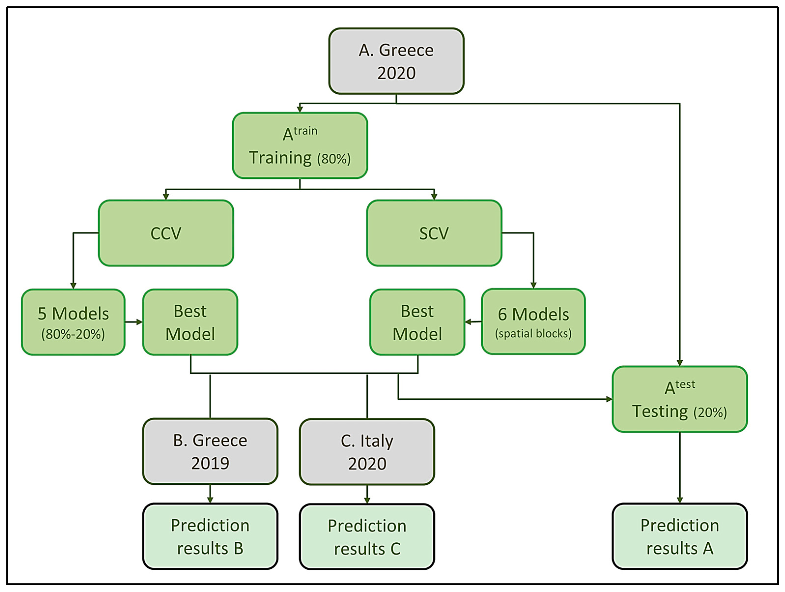
2.2. Research Workflow

To assess the CCV and SCV resampling methods in the current study, the A dataset (Greece, July/2020) was used as a reference, from which different ML models were produced. Initially, the specific dataset was randomly split into training (A^train: 80% of A) and testing (A^test: 20% of A) datasets. The training dataset was split using two resampling methods (CCV or SCV), and different ML models were trained using QRF, RF, and GBM algorithms. The testing dataset was used for assessing the ML model’s results (Figure 3).

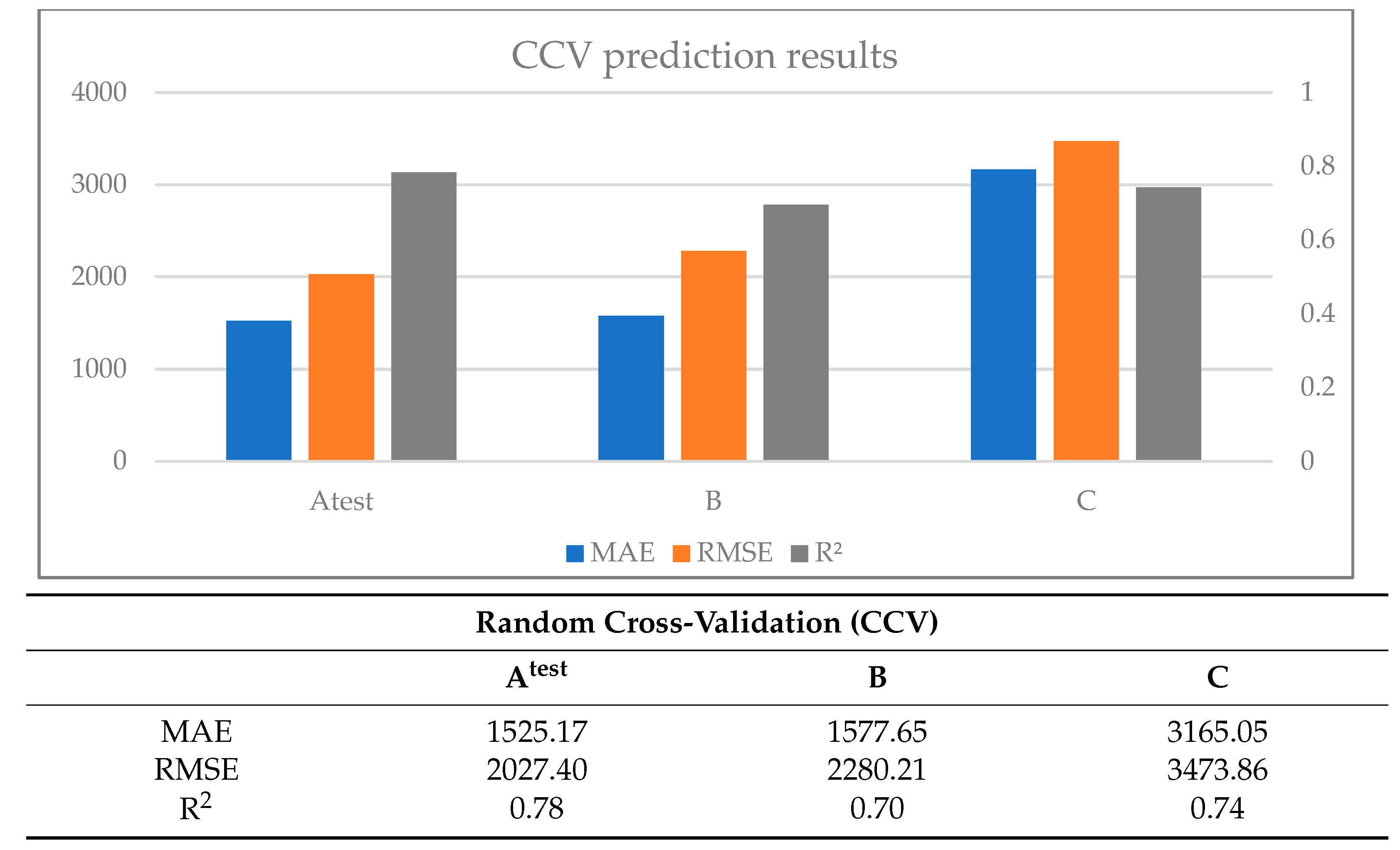
In more detail, in the case of CCV, a 5-fold cross-validation was performed for each ML algorithm, and the best model per algorithm was used for estimating the EC in the A^test (20% of Greece, 7/10), B (Greece, 6/19) and C (Italy, July/2020) datasets.

Regarding spatial cross-validation (SCV), the training dataset was split using spatial blocks (6 folds) with optimum block sizes that were calculated by utilizing the median of the covariates’ spatial autocorrelation ranges. The same ML models (QRF, RF, and GBM) as in the CCV case were developed and evaluated. The prediction accuracy of the best ML models for each ML algorithm was also assessed using the testing (A^test), B, and C datasets. Finally, all the results from the SCV were compared with the corresponding results from the CCV.

2.3. Environmental and Soil Covariates

The groundwater samples were collected from a variety of locations that were dispersed throughout the study area to obtain a comprehensive understanding of the water quality in the region. Even though there were data from multiple timeframes, only the data from specific years (2020 and 2019) were chosen. The samples were then analyzed in a laboratory using a range of tests and techniques to determine the levels of various contaminants and indicators of water quality. Specifically, the covariates that were measured were electric conductivity (EC) temperature (C), bicarbonate (HCO₃⁻), nitrate (NO₃⁻), pH, potassium (K⁺), sulphate (SO₄²⁻), distance from sea (dist), and x, y coordinates (

Table 1. Environmental and soil covariates that were used in the study.

	Covariates	Unit	Method
1	Electric conductivity (EC)	μs/cm	Measured in situ using the YSI ProDSS Multiparameter portable equipment
2	Temperature	C	Measured in situ using the YSI ProDSS Multiparameter portable equipment
3	Bicarbonate (HCO3−)	mg/L	Measured in the lab using the titration method with neutralization of HCl
4	Nitrate (NO3−)	mg/L	Measured in the lab using spectrophotometer
5	pH	-	Measured in the lab using electrodes
6	Potassium (K+)	mg/L	Measured in the lab using a flame photometer
7	Sulphate (SO42−)	mg/L	Measured in the lab using spectrophotometer
8	Distance from sea (dist)	meters	Calculated from the coordinates
9	x	meters	Coordinates estimated from data
10	y	meters	Coordinates estimated from data

).

Based on the descriptive statistics (

Table 2. Descriptive statistics of auxiliary variables from the 147 locations in Area A.

	EC	Temp	HCO3−	NO3−	pH	K+	SO42−	dist
mean	4104.43	22.19	257.28	18.45	7.44	4.65	85.17	4374.28
sd	4289.03	2.21	104.53	27.29	0.44	4.28	105.37	2867.18
median	2520	21.7	244.8	8.86	7.43	3.5	49.95	3575.12
min	240	18.3	37.5	0	5.61	0.7	2.5	312.38
max	23,000	28.8	1049.2	157	8.55	25.82	816	13,326.55
skew	1.95	0.77	4.71	2.74	−0.07	2.78	3.42	1.17
kurtosis	4.03	0.21	31.5	8.44	1.17	8.52	16.37	0.84

,

Table 3. Descriptive statistics of auxiliary variables from the 65 locations in Area B.

	EC	Temp	HCO3−	NO3−	pH	K+	SO42−	dist
mean	3701.75	22.34	227.14	13.7	7.66	3.46	98.74	5295.45
sd	3762.52	1.99	65.11	19.54	0.45	2.69	122.04	2932.52
median	1650	22	237.7	7.5	7.6	2.5	45.15	4822.94
min	290	19	84.18	0.1	7	0.76	9.1	598.71
max	15,500	27	396.5	121.5	9.27	14.1	651.3	11,146.83
skew	1.24	0.31	0.04	3.29	0.82	1.94	2.19	0.46
kurtosis	0.65	−0.43	0.56	13.3	0.83	4.28	5.39	−0.95

and

Table 4. Descriptive statistics of auxiliary variables from the 107 locations in Area C.

	EC	Temp	HCO3−	NO3−	pH	K+	SO42−	dist
mean	2381.61	18.21	320.09	23.7	7.38	16.61	101.16	9420.69
sd	2690.69	1.58	80.41	23.92	0.28	21.78	122.81	6084.44
median	1079	18.04	307	22.6	7.4	6.7	44	9691.41
min	342	14.3	90.92	0	6.8	0.9	8	0
max	11,643	22.5	600	197.95	8.25	130	504.32	23,302.7
skew	1.78	0.06	0.69	3.76	0.6	2.42	1.73	−0.05
kurtosis	2.2	−0.11	1.67	24.27	0.71	6.81	2.2	−1.11

) it is obvious that the three areas have similar characteristics. Their temperature is comparable with a mean value of 22.19 °C for Area A, 22.34 °C for Area B, and 18.21 °C for Area C, and all areas are close to the sea with mean distance values of the sample locations 4.3 km for Area A, 5.2 km for Area B, and 9.4 km for Area C. Other parameters are also quite close, such as the EC mean values of 4104.43 μs/cm, 3701.75 μs/cm, 2381.61 μs/cm, and pH mean values of 7.44, 7.66, 7.38 for A, B, and C, respectively.

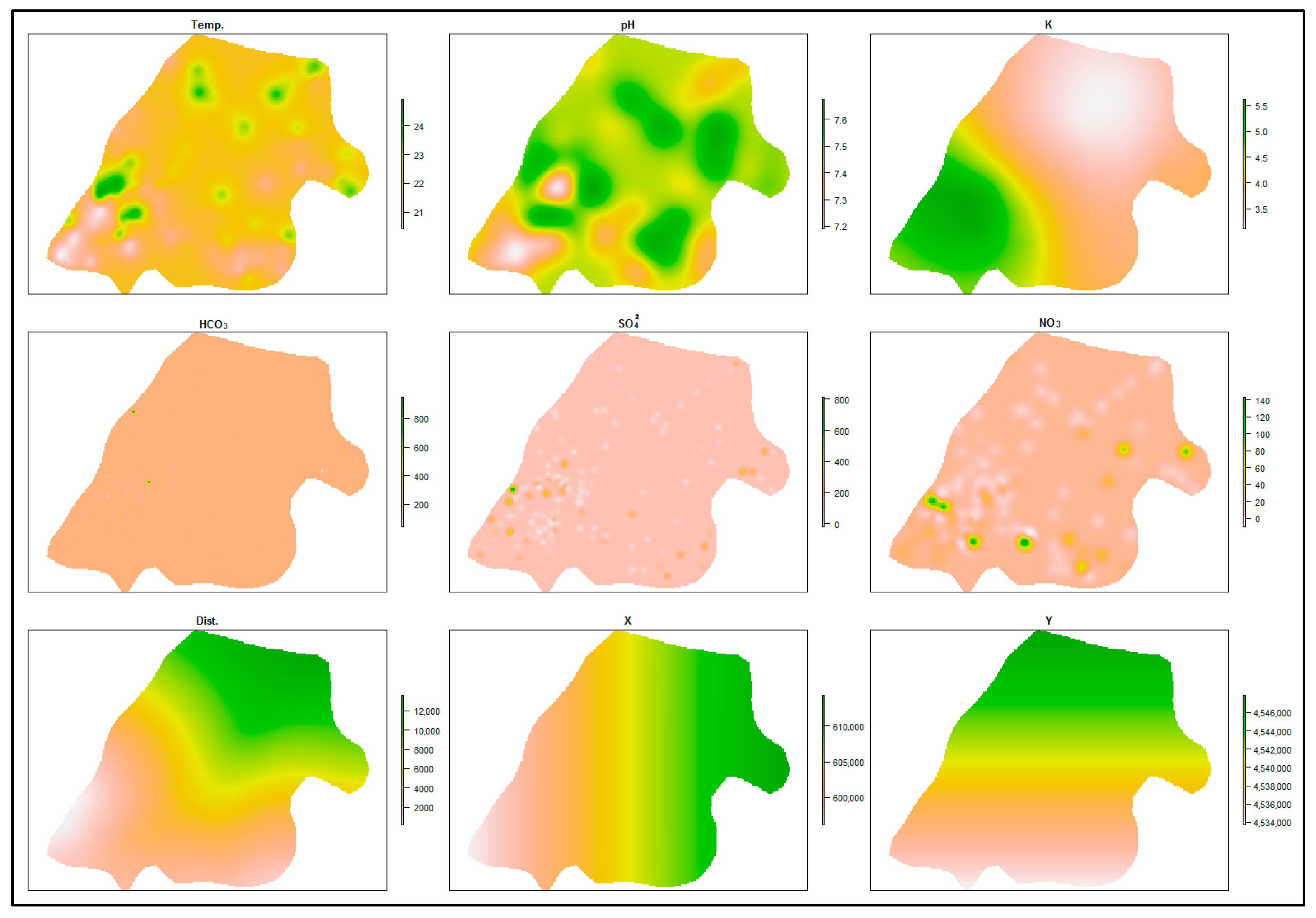
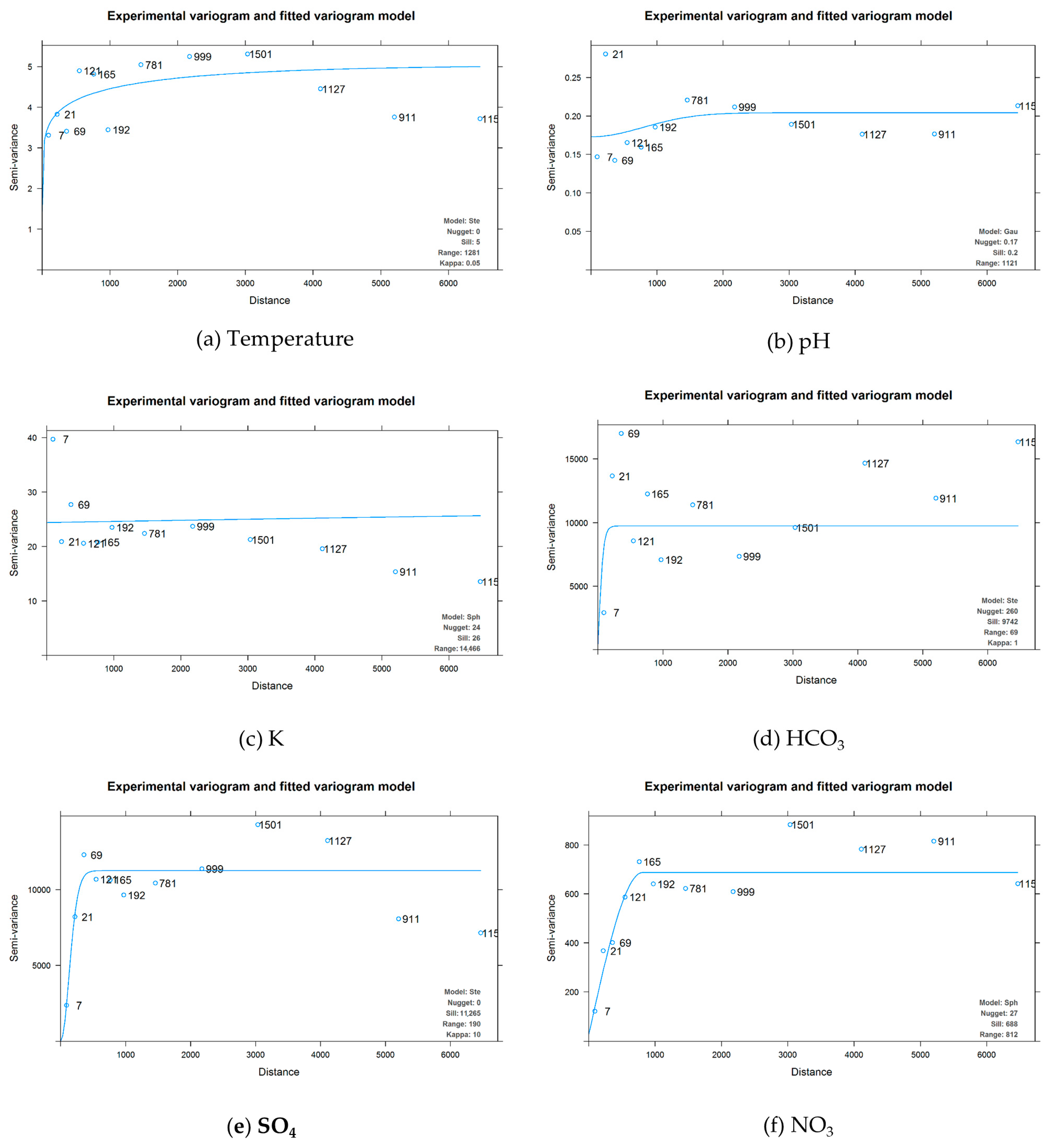
The spatial distribution of the covariates for the overall area was estimated using ordinary Kriging interpolation (OK) to calculate their spatial autocorrelation range (Figure 4).

The empirical semivariograms of the variables Temperature, HCO₃⁻, SO₄²⁻, and NO₃⁻ revealed spatial autocorrelation, as seen by low semi-variance values at near distances and low nugget-to-total-sill ratios (Figure 5). Especially SO₄²⁻ and NO₃⁻ appear to have the strongest autocorrelation with short ranges. Distance from the sea, x, and y did not exhibit spatial autocorrelation, so their empirical semivariograms were omitted.

2.4. Cross-Validation

Most of the ML studies utilize standard random cross-validation (CCV) as the preferred resampling method due to its ability to provide a bias-reduced assessment of the models’ capabilities to generalize the learned relationship to unknown data. However, this statement assumes that the data are independent and identically distributed. In the case of spatial data, this assumption might be violated due to the spatial autocorrelation of the data.

As a result, different strategies are presented under the umbrella term “spatial cross-validation” (SCV) to overcome this issue. Block CV [12] is one of them, in which the dataset is divided into numerous folds with matching geographical locations, resulting in spatially homogeneous clusters of observations [37]. These clusters, which may be formed by rectangles, polygons, or other custom geometries, are used as cross-validation training, and testing datasets. Another approach is known as “buffered CV”, and like the well-known “leave-n-out CV”, it incorporates distance-based buffers around hold-out points to remove training observations in a neighboring circle [12,16,19,38].

However, whether and to what extent SCV is effective is not straightforward and is dependent on several factors, including the prediction area (interpolation-extrapolation), the spatial autocorrelation of the landscape (long-sort autocorrelation ranges of predictors), the sampling pattern (regular-clustered distributed training samples), and the geographical prediction space (distances from prediction locations to its nearest training samples) [18]. Wadoux et al(2021) [39] even claim in their study that “…spatial cross-validation strategies resulted in a grossly pessimistic map accuracy assessment and gave no improvement over standard cross-validation”.

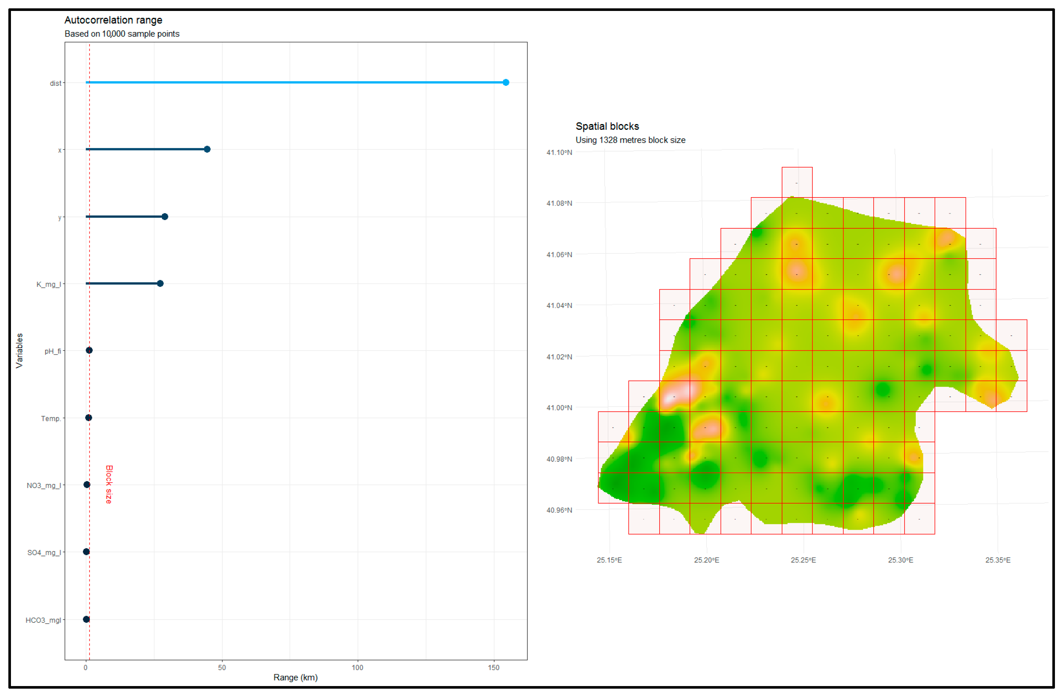
The optimum size of blocks or buffers to use in the spatial cross-validation procedures is one of the main concerns. The size needs to be sufficient to eliminate autocorrelation in the data, but not excessively so that the training dataset and testing dataset are too far apart and inadvertently lead to an extrapolation [12]. The spatial autocorrelation range in the model residuals may be used to estimate the ideal block size [40]. To obtain the residuals, though, this necessitates fitting the model first. Using the auxiliary variables’ existing autocorrelation instead as a rough indicator before model fitting is a simpler approach [19].

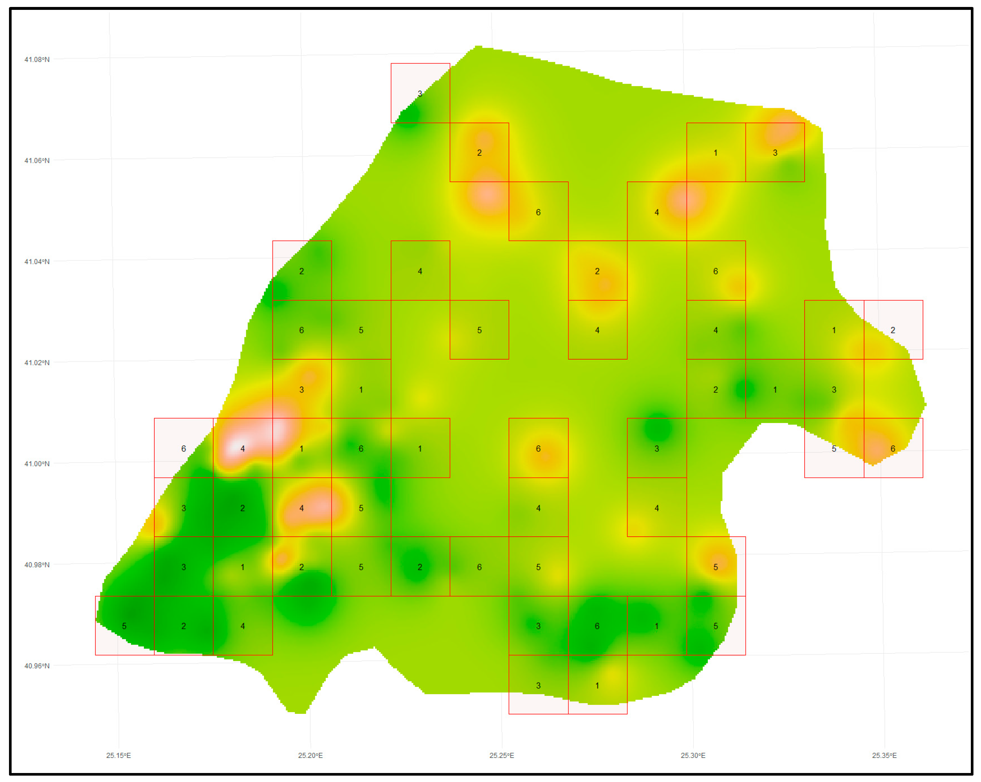
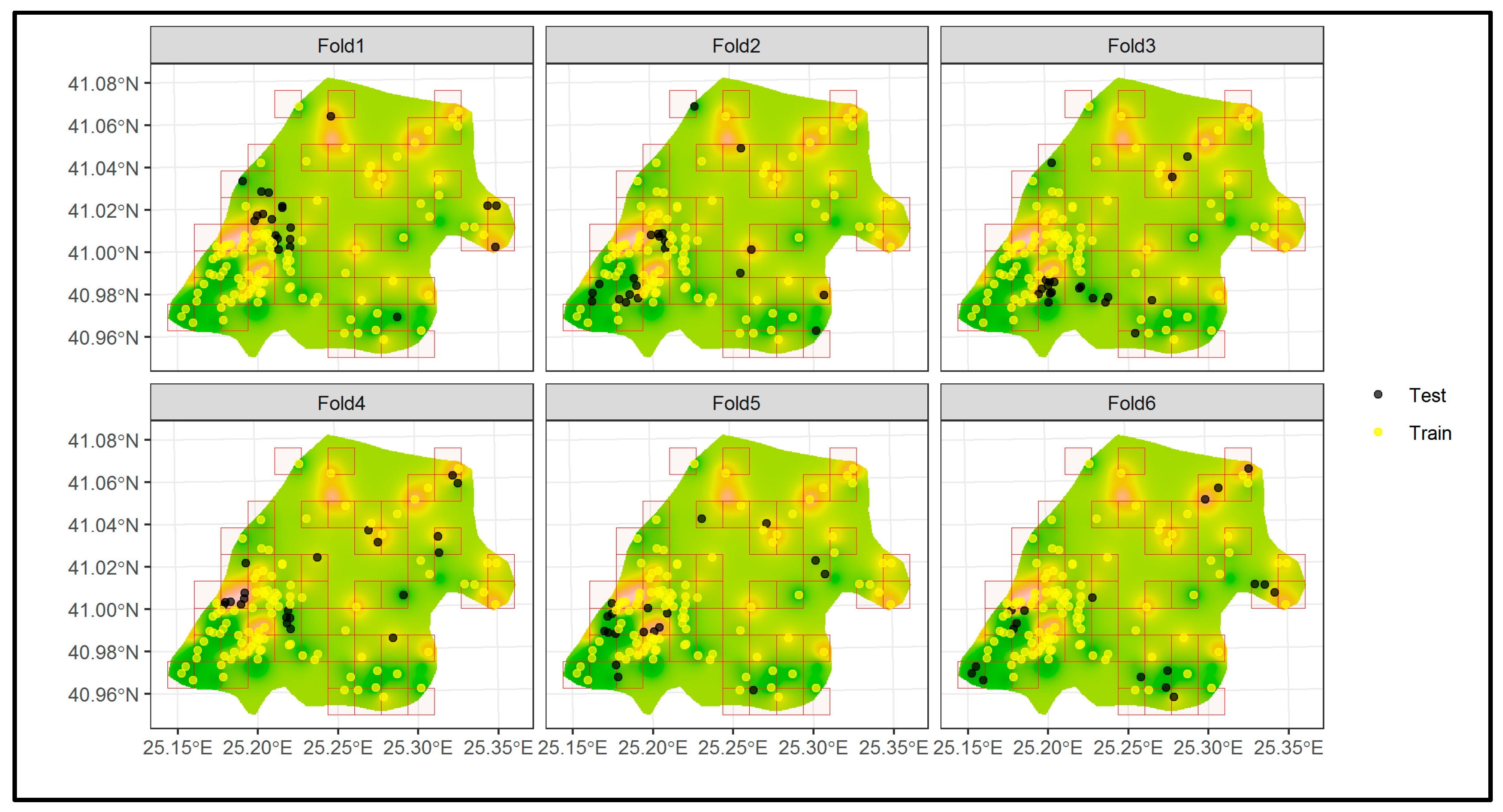
The BlockCV package in R [19] was utilized to apply SCV for the current study. Several methods for constructing spatial blocks are provided by the BlockCV package, including creating user-defined spatial polygons, square spatial blocks of a certain size, and vertical/horizontal bins with specific heights and widths. Additionally, it offers a tool to examine the spatial autocorrelation in the predictors and enables the placement of blocks into folds in a random, systematic, or checkerboard way. This is accomplished by automatically fitting variogram models to each predictor and determining the spatial autocorrelation’s effective range. The optimum SCV block, or buffer size, is estimated using the median of the predictors’ spatial autocorrelation ranges. In the current study, the spatial blocks were assigned to the training dataset (A^train), which is 80% of the A dataset (119 points), in random order. The spatially separated folds (six folds) were used to assess the different ML models per ML algorithm (

Table 5. Number of sample points in training and testing datasets for SCV (left) and CCV (right).

SCV			CCV
Folds	Training	Testing	Folds	Training	Testing
1	99	20	1	96	23
2	97	22	2	96	23
3	101	18	3	96	23
4	98	21	4	96	23
5	103	16	5	96	23
6	97	22

). The number of folds was chosen to divide the dataset into approximately 80% for training and 20% for testing, similar to CCV. The model with the lowest RMSE for each algorithm was used for the assessment of the water EC in the A^test (20% of Greece, 7/10), B (Greece, 6/19), and C (Italy, 7/2020) datasets.

In the instance of CCV, the initial training dataset (A^train) was utilized to train five (5) separate ML models per ML algorithm using a five-fold cross-validation technique (Table 5). The best ML model for each algorithm, based on the RMSE, was used to predict the EC in the A^test (20% of Greece, 6/20), B (Greece, 6/19), and C (Italy, July/2020) datasets.

2.5. ML Methods (Random Forest, Quantile Random Forest, Gradient Boosting)

Different commonly utilized ML algorithms like Random Forest, Quantile Random Forest, and Gradient Boosting were employed in the current study.

Random Forest is an ensemble learning method that makes predictions using multiple decision trees [41]. It is a type of bagging algorithm, which aggregates the predictions of multiple decision trees to reduce variance and enhance the model’s overall accuracy. The basic idea behind Random Forest is to take a sample of the data, fit a decision tree to each sample, and then get the final prediction by averaging the predictions of all the trees.

Random Forest’s main advantage is that it can handle high-dimensional and complicated data sets and is relatively tolerant of outliers and irrelevant features [42]. In addition, Random Forest models are easy to evaluate because feature importance can be calculated based on the average impurity decrease across all trees [41].

The number of decision trees in the ensemble is one of the main hyperparameters for Random Forest. Generally, a larger number of trees improves performance but requires more computational resources [43]. Another important hyperparameter is the number of features considered at each split. A larger number of features results in more complicated trees, but also increases the risk of overfitting. The focus of the current study was to assess the different ML models created either from CCV or SCV, not their optimization. Therefore, default or commonly used values were used as hyperparameters of the ML models (

Table 6. RF and QRF hyperparameters.

Hyperparameters	Description	Values Used
mtry	The number of random features used in each tree.	3
num.trees	The number of grown trees.	1500
min.node.size	Minimal node size.	5
splitrule	A switch for linear output units.	extratrees

).

Quantile Random Forest is an extension of the Random Forest method that includes the estimate of quantiles and the median, in addition to the mean of the response variable [44]. Random Forest models estimate the mean of the response variable by default; however, in some cases, it is more important to know the response variable’s quantiles. Their hyperparameters are the same as RF’s.

Gradient Boosting is another ensemble learning technique that predicts by combining multiple weak learners [45]. Gradient Boosting differs from Random Forest in that it uses a series of decision trees, with each tree attempting to correct the errors of the prior tree [45]. This is accomplished by fitting a decision tree to the loss function’s negative gradient. The final prediction is the sum of all the trees’ predictions. Gradient Boosting is suitable for regression and classification problems with a small amount of data or a high-dimensional feature space [46]. Gradient Boosting can manage non-linear correlations between characteristics and target variables, which is one of its primary advantages [46].

In the current study, we used the gbm (generalized boosted regression models) package (Section 2.7) that includes regression methods for least squares, absolute loss, t-distribution loss, quantile regression, logistic, multinomial logistic, Poisson, Cox proportional hazards partial likelihood, AdaBoost exponential loss, Huberized hinge loss, and Learning to Rank measures (i.e., LambdaMart).

The basic hyperparameters of gbm are the following (

Table 7. gbm hyperparameters.

Hyperparameters	Description	Values Used
n.trees	Total number of trees to fit.	100
interaction.depth	Maximum depth of each tree.	1
shrinkage	Learning rate	0.1
n.minobsinnode	Minimum number of observations in the terminal nodes of the trees.	10

): The “n.trees” which is an integer, specifies the total number of trees to fit. This is equivalent to the number of iterations and the number of basic functions in the additive expansion. The “interaction.depth” specifies the maximum depth of each tree (i.e., the highest level of variable interactions allowed). The “shrinkage” is a parameter applied to each tree in the expansion, also known as the learning rate or step-size reduction. A smaller learning rate typically requires more trees and usually gives improved predictive performance. Finally, there is the “n.minobsinnode”, which is an integer specifying the minimum number of observations in the terminal nodes of the trees. In all cases, the default values were used as hyperparameters.

2.6. Error Assessment

The prediction accuracy of the different ML models was measured by the difference between the observations and the predictions in the A^test, B, and C datasets. The following metrics were used to assess the results (

Table 8. Statistical metrics to assess model performance.

Metrics	Equation
Mean absolute error (MAE)	$MAE=\frac{{{\displaystyle \sum }}_{i=1}^n\left|\widehat{z}\left(s_i\right)-z\left(s_i\right)\right|}{n}$	(1)
Root mean square error (RMSE)	$RMSE=\sqrt{\frac{{{\displaystyle \sum }}_{i=1}^n{\left[\widehat{z}\left(s_i\right)-z\left(s_i\right)\right]}^2}{n}}$	(2)
Coefficient of determination (R2)	$R^2=\frac{SSE}{SSTO}$	(3)

).

To evaluate the performance of the models, several statistical metrics were used. The mean absolute error (MAE) was calculated first, which expresses the average-model-prediction error based on the measured value $z\left(s_i\right)$ and its prediction $\widehat{z}\left(s_i\right)$ in $s_i$ locations of the samples, as seen in Equation (1). Additionally, the root mean square error (RMSE) was employed, which provides an estimate of the standard deviation of the residuals (prediction errors), defined by Equation (2). Finally, the coefficient of determination (R²) was used, which represents the amount of variation explained by the model (Equation (3)). The SSE represents the sum of squares of errors and SSTO the total sum of squares. The R² ranges from 0 to 1, with 0 indicating that no variation is explained by the model and 1 indicating that all variation is explained by the model, indicating a perfect model. Lower values for RMSE and MAE are associated with greater predictive accuracy.

2.7. Software

The statistical software R (version 4.2.0) was used for the statistical analyses. The gstat package [47] was utilized for geostatistical analysis, the gbm package [48] for gradient boosting, the ranger package [49] was utilized for RF and QRF, and the BlockCV package [19] for spatial cross-validation (SCV). The distance from sea was calculated using the Saga software version 7 [50].

3. Results

3.1. Spatial Cross-Validation Parameters

A BlockCV function that assesses the spatial autocorrelation in the covariables was utilized to determine the SCV block size. This operates by fitting variogram models to each continuous raster automatically and determining the effective range of the spatial autocorrelation [19]. The approximate recommended ideal block size for SCV is the median value of the covariate ranges for each location. This is the range over which observations are independent. The use of the median value instead of the mean ensures that the block size will have a reasonable value regardless of a possible huge autocorrelation range.

In the current study, based on 10,000 sample points across the area, this median value was estimated at 1328 m; therefore, 1400 m was used as the block size for the SCV (Figure 6).

Each block was allocated a number ranging from 1 to 6 (Figure 7). Spatial cross-validation was carried out by excluding data from blocks with a certain number (the testing dataset) and utilizing the remaining data from the other blocks as the training dataset. This was done six times, once for each number (1–6), using the default hyperparameters for each ML method (Figure 8).

3.2. Prediction Results

The full prediction results of the ML models for the different datasets are presented in

Table 9. Prediction results for water EC with random cross-validation (CCV) and spatial cross-validation (SCV). With an asterisk, the best value in each dataset (A^test, B, or C) for the specific ML algorithm. (A^test. Greece, summer 2020; B. Greece, summer 2019; C. Italy, 2020).

Random Cross-Validation (CCV)				Spatial Cross-Validation (SCV)
MAE	Atest	B	C	MAE	Atest	B	C
QRF	1281.21 *	1448.58	2863.62 *	QRF	1406.64	1400.77 *	2950.98
RF	1599.26 *	1471.58	4317.37	RF	1605.28	1458.08 *	4075.10 *
GBM	1695.03 *	1812.79	2314.16	GBM	2100.54	1742.41 *	2258.93 *
RMSE	Atest	B	C	RMSE	Atest	B	C
QRF	1970.74 *	2338.38	3169.33	QRF	2093.53	2064.84 *	3150.68 *
RF	2076.43 *	2040.39	4487.96	RF	2143.72	1931.51 *	4244.82 *
GBM	2035.02 *	2461.85	2764.29	GBM	2477.75	2211.24 *	2704.68 *
R2	Atest	B	C	R2	Atest	B	C
QRF	0.788	0.714	0.778	QRF	0.790 *	0.728 *	0.828 *
RF	0.790 *	0.717	0.827 *	RF	0.772	0.757 *	0.826
GBM	0.771 *	0.654	0.622	GBM	0.658	0.680 *	0.624 *

.

The cross-validation resampling method that was done with a random split (CCV) produced the best results in the A^test dataset, slightly worse in the B dataset (same area, another time), and much worse for the C dataset from another location. Specifically, the mean MAE, mean RMSE, and mean R² for predicting EC in the A^test dataset were 1525.17, 2027.40, and 0.783 and whereas for predicting EC in the B dataset, the means were 1577.65, 2280.21, and 0.695, and in the C dataset 3165.05, 3473.86 and 0.743, respectively (Figure 9).

Between the different ML models, the QRF had better results and GBM worse; however, due to a lack of hyperparameter optimization, we cannot compare the different ML algorithms. Tuning the hyperparameters may produce better results in general. The high RMSE and MAE values for the C dataset suggest that the specific ML models should not be used for predicting values in another area.

The spatial cross-validation resampling method produced slightly better results in the B dataset (of the same area at another time) than in the A^test dataset (testing dataset, same area, same place), and much worse results in the C dataset from another place. This is noteworthy because ML models usually have the best results in the testing dataset and much worse in other new ones. In more detail, the mean MAE, mean RMSE, and mean R² for predicting EC in the A^test were 1704.16, 2238.34, and 0.74, whereas for predicting EC in the B dataset, the means were 1533.75, 2069.20, and 0.72, and in the C dataset 3095.00, 3366.73 and 0.76, respectively (Figure 10).

Comparing the two distinct resample strategies of CCV and SCV (Figure 11), the SCV ML models performed better with new data (B and C datasets), despite not having the best results with the testing dataset. Specifically, for the A^test dataset the mean prediction results for CCV and SCV, were 1525.17 vs. 1704.16 for MAE, 2027.40 vs. 2238.34 for RMSE, and 0.78 vs. 0.74 for R². For the B dataset, the mean prediction results for CCV and SCV were 1577.65 vs. 1533.75 for MAE, 2280.21 vs. 2069.20 for RMSE, and 0.70 vs.0.72 for R². Finally, for the area of Italy (C) the mean prediction results for CCV and SCV were 3165.05 vs. 3366.73 for MAE, 3473.86 vs. 3366.73 for RMSE, and 0.74 vs.0.76 for R².

This could be explained by the fact that SCV attempts to minimize the spatial autocorrelation bias in the training dataset, leading to poorer prediction competence than the CCV in the testing dataset (A^test) but improved prediction results in new datasets (better generalization capabilities).

4. Discussion

Machine learning algorithms have been employed in several types of research with excellent prediction accuracy. Nevertheless, these outcomes are occasionally excessively optimistic, making models appear more accurate and reliable than they are. Overfitting capabilities of the ML methods, along with inadvertent biases, might result in extremely modest prediction errors in the testing dataset but not the same outstanding results in new data, limiting the model’s capacity to generalize the learned connection to independent data.

Spatial data are a special kind of data that might introduce biases to ML models due to their intrinsic spatial autocorrelation. To address this issue, a resampling method called spatial cross-validation has been used lately that splits the data into spatially disjoint subsets, blocks, or buffers, which are subsequently used in ML.

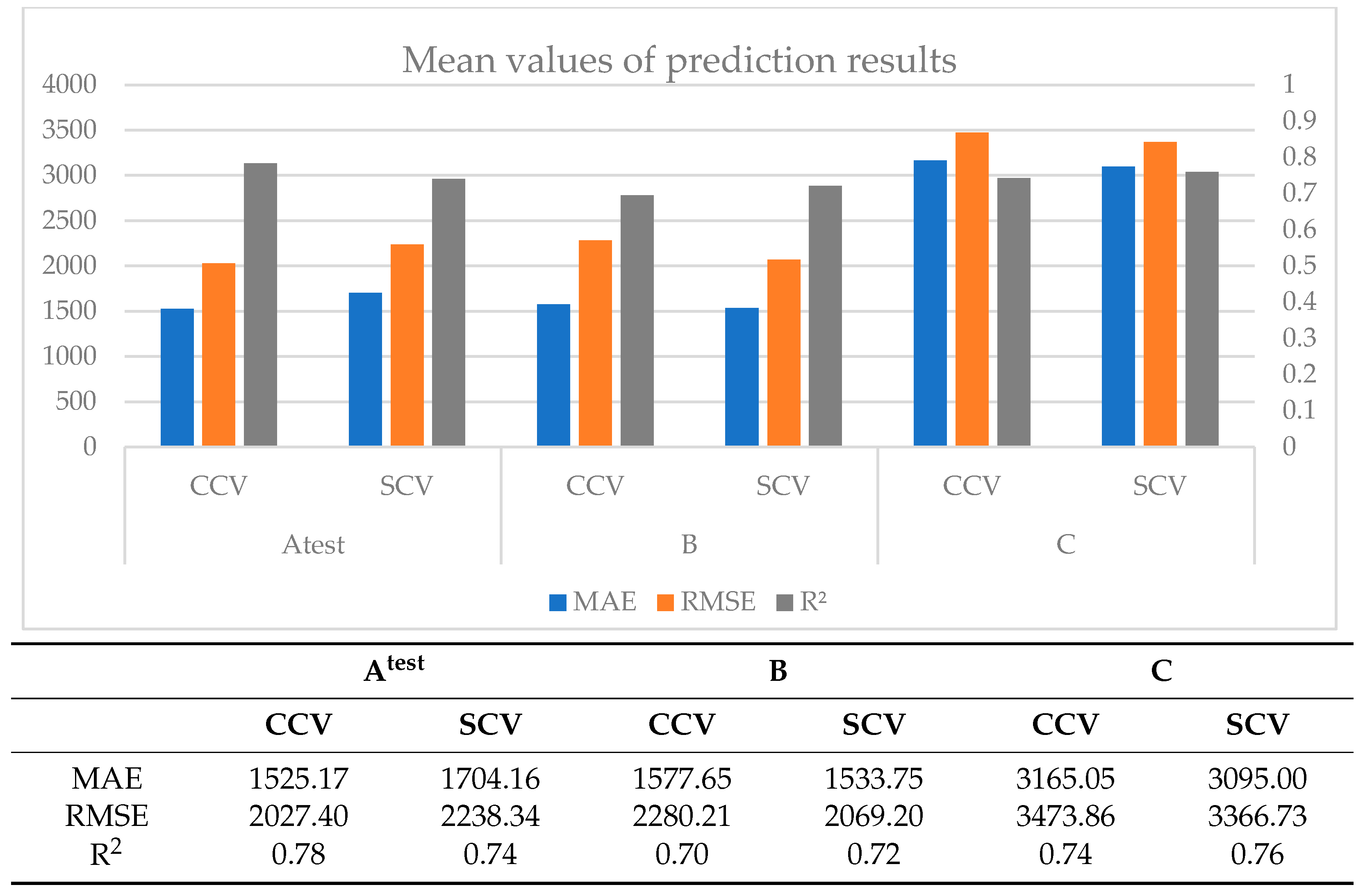
In the current study, two resampling methods are utilized and assessed, which are conventional random cross-validation (CCV) and spatial cross-validation (SCV). These methods were used to create ML models with a training dataset and assess their performance in predicting groundwater EC in a testing dataset (same area, same time) and new, unseen data from a different place or a different time.

Based on the results, models developed with random cross-validation (CCV) demonstrated superior predictive accuracy within the testing dataset. However, their performance could have been better when applied to totally new data from a different time or different location. This is in line with prior research indicating that CCV often leads to models prone to overoptimistic and biased prediction results [9,17,51]. The SCV method produced worse results in the testing dataset than in the new B dataset (same area, another time). In the case of the C dataset, the results were the poorest.

When CCV and SCV are compared, we can see that the ML models built by SCV performed better on new unknown data (the B and C datasets) than the CCV. The SCV captures the spatial patterns in the data while also reducing the over-optimism bias (i.e., the improved prediction results of CCV in the testing dataset) often associated with standard cross-validation methods. Considering space in the resampling algorithm provides ML models with superior generalization capabilities for new unknown data (in both new space and time).

Apart from that, we could mention that the models that were created from the initial dataset performed overall adequate in the testing dataset (A^test) and the dataset from the same area from a different time (B), but not so well in the dataset from a different area with similar characteristics (C). As a result, it is not recommended to utilize (the specific) ML models to estimate groundwater EC in new locations, even if they exhibit similar properties. Ideally, customized models should be created for different locations that are optimized for the specific area and the specific parameters. Nevertheless, be cognizant that we did not optimize the model’s hyperparameters in the study, so a possible improvement of the models, in general, is very probable.

The results suggest that when working with spatial data, it is recommended to employ SCV in conjunction with ML. Even when aiming to develop tailored models for a particular area, SCV offers ML models with enhanced temporal generalization abilities, leading to improved future prediction results. These findings underscore the importance of carefully evaluating and considering factors such as location when utilizing ML models for predictive purposes. In future research, it would be beneficial to explore alternative SCV methods and their impact on the accuracy of ML predictions, as well as examine how spatial autocorrelation affects the optimization of ML hyperparameters.