
Investigating the Effects of Climate and Land Use Changes on Rawal Dam Reservoir Operations and Hydrological Behavior
 ,
,  ,
,  , ,
, , 

Abstract
:1. Introduction
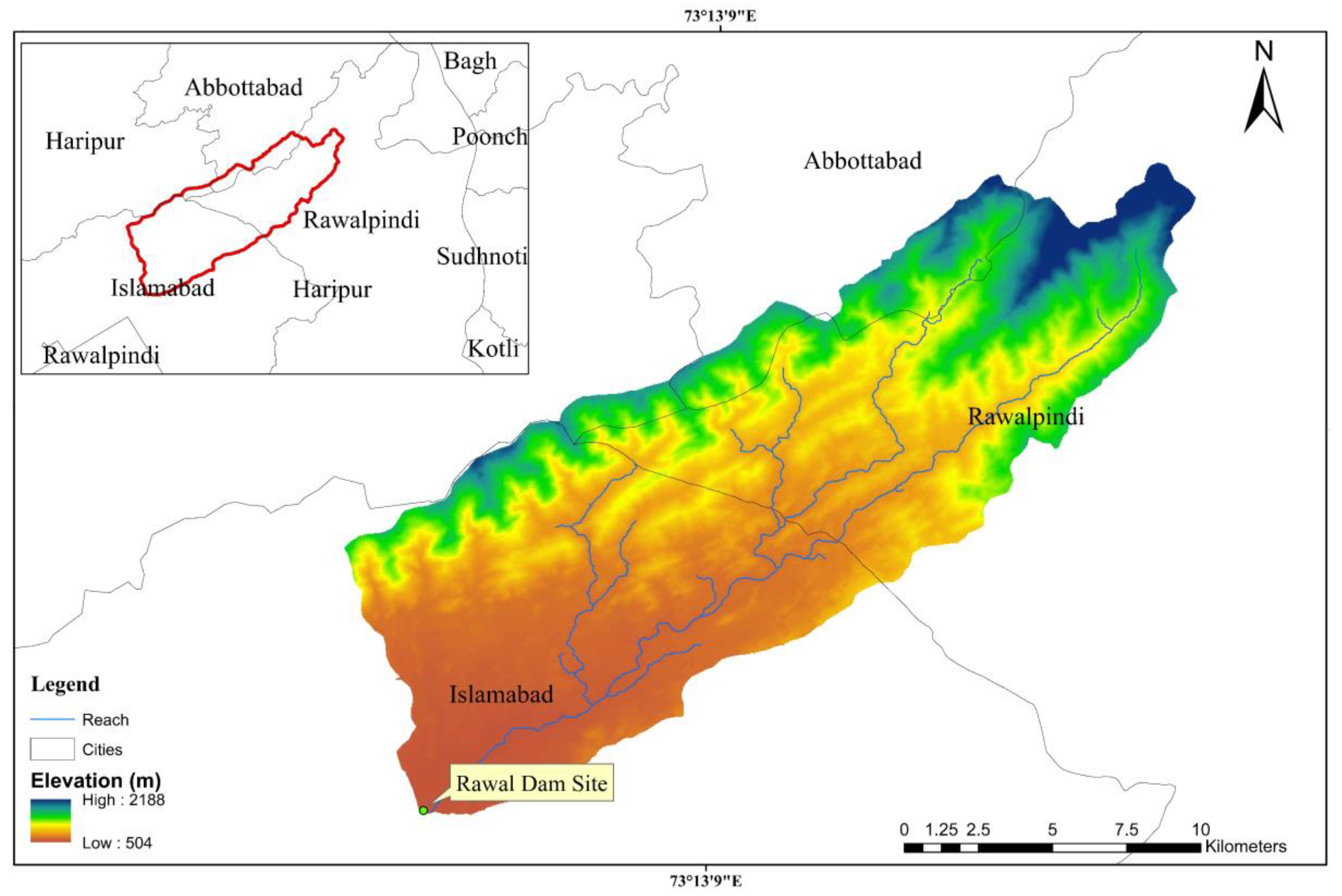
2. Study Area
3. Materials and Methods
3.1. Datasets
3.1.1. Hydro-Meteorological Data
3.1.2. Remote Sensing Data
3.1.3. Climate Projected Data
3.2. Methodology
3.2.1. Statistical Downscaling
3.2.2. Image Classification
3.2.3. Hydrological Modeling
3.2.4. Model Performance Evaluation
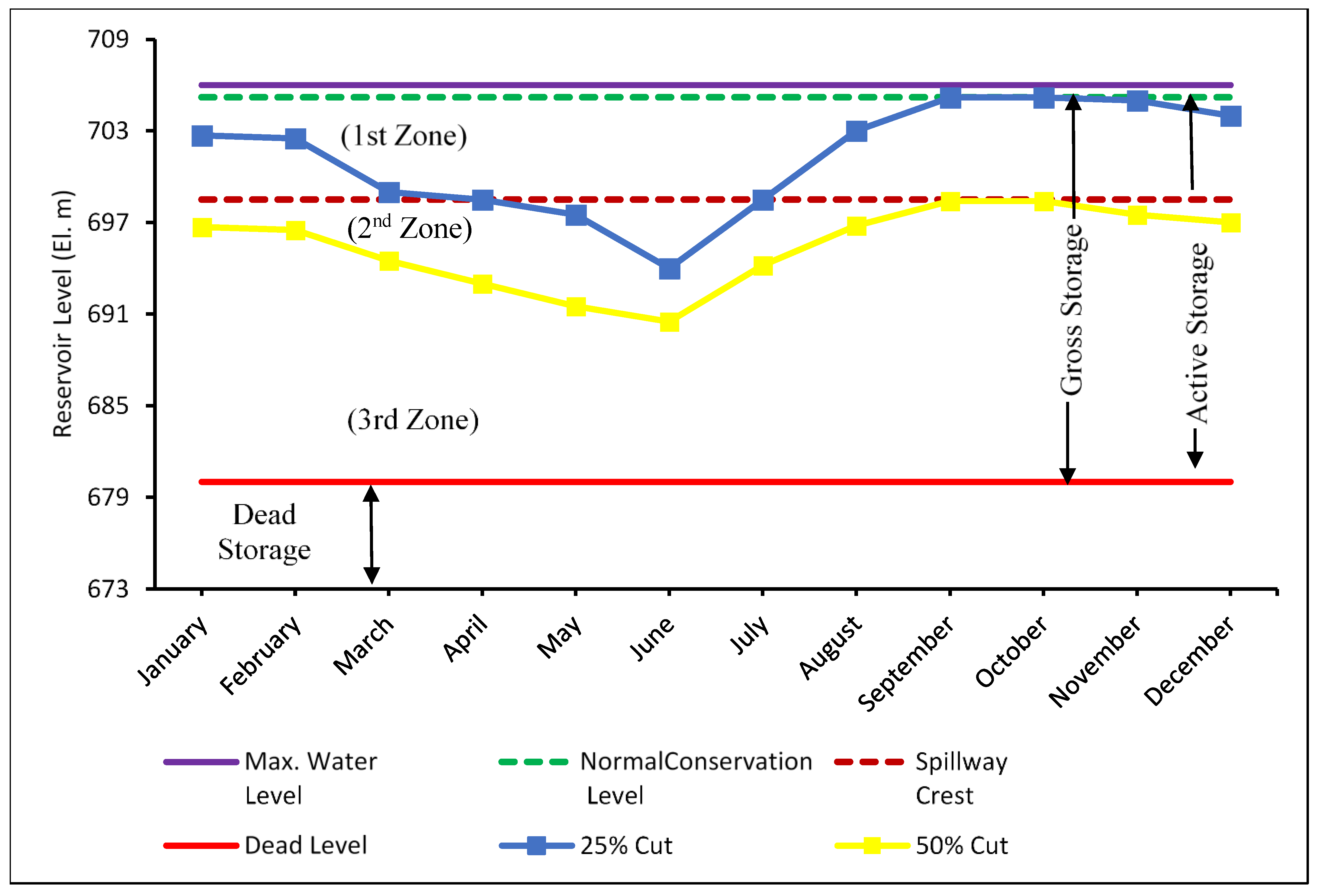
3.2.5. Model for Reservoir Simulation Application (HEC-ResSIM)
4. Results
4.1. Downscaling of Future Climate Data
4.2. Potential Shifts in Rainfall and Temperature
4.2.1. Projection of Mean Maximum Temperature
4.2.2. Projection of Mean Minimum Temperature
4.2.3. Projection of Precipitation
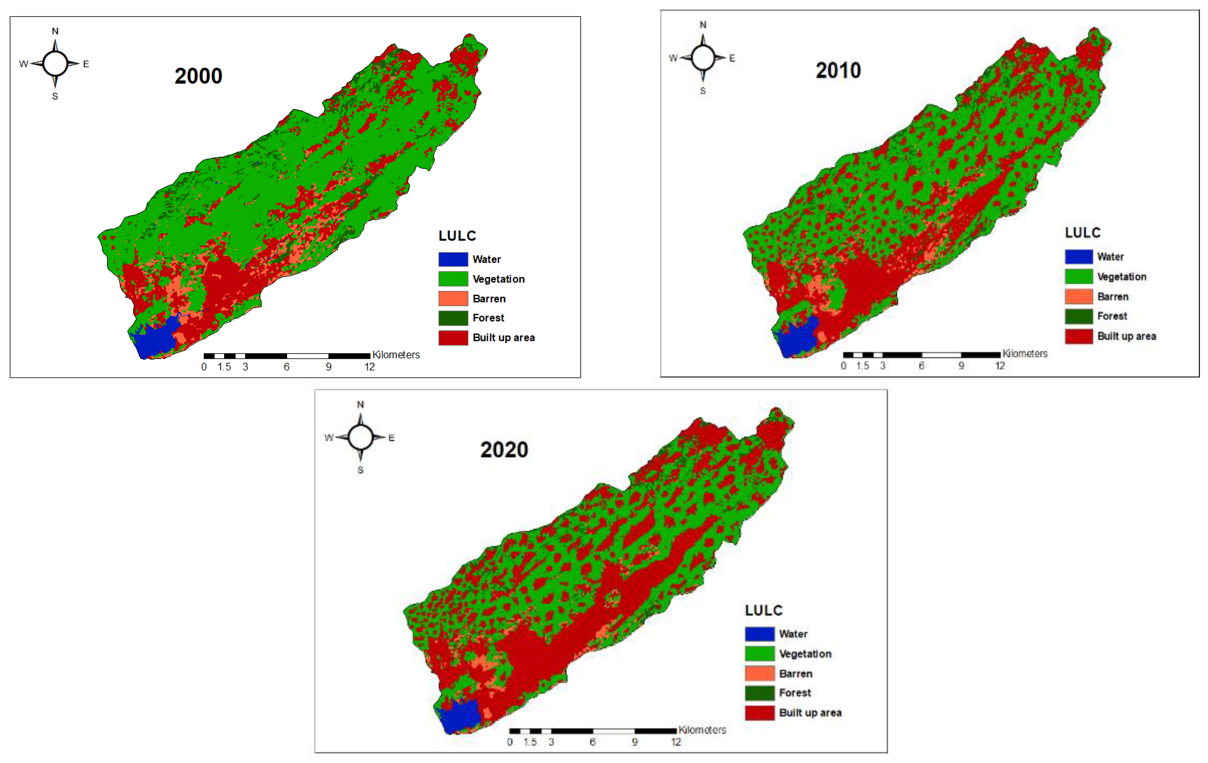
4.3. Land Use Land Cover Change Trends
Projected Land Use Land Cover
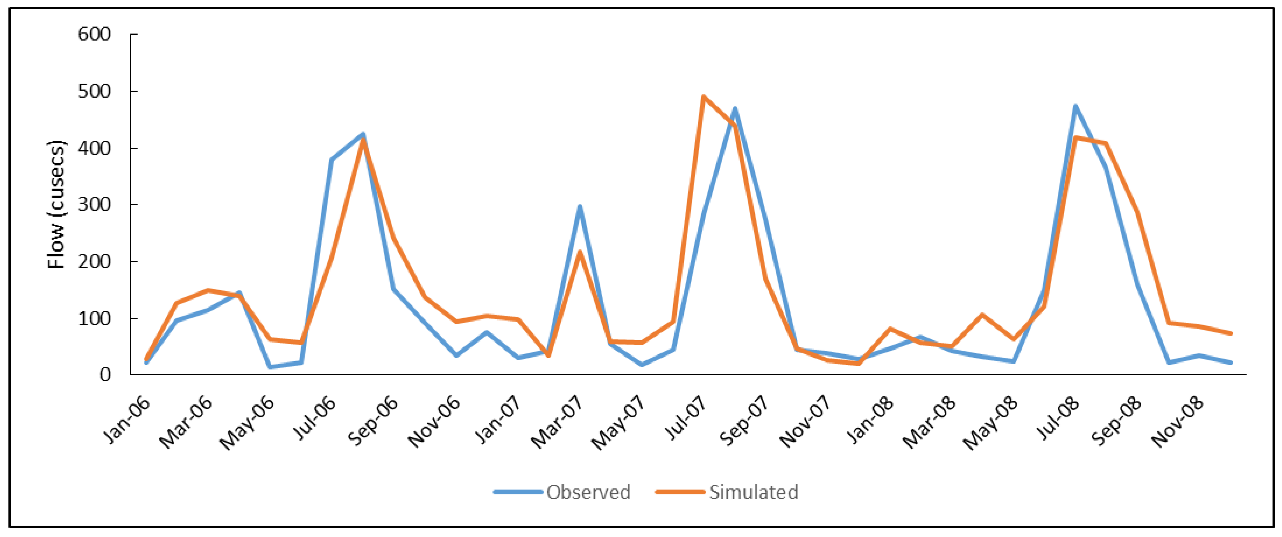
4.4. Calibration and Validation of Hydrological Model
4.5. Impact of Projected Climate on Flows
4.6. Reservoir Operation Simulation
Impacts of Climate Change on Reservoir Operational Strategy
5. Discussion
6. Conclusions
- In comparison to the baseline period (1990–2015), the Rawal Dam catchment’s annual minimum, maximum, and mean temperatures and precipitation have been rising steadily since 2016. Future streamflows are influenced by the higher precipitation.
- Under current land use and land cover conditions, it is expected that the average daily streamflow at Rawal Dam will rise from 129.5 cusecs (1990–2015) to 151.9 cusecs under SSP2 and to 160.5 cusecs under SSP5.
- While this flow grew from 129.5 cusecs (1990–2015) to 177.1 cusecs under current climate conditions and future land use and land cover scenarios.
- The findings showed that while mean monthly flows have risen overall, those for December and February have decreased.
Author Contributions
Funding
Data Availability Statement
Conflicts of Interest
References
- Higashi, H.; Dairaku, K.; Matsuura, T. Impacts of Global Warming on Heavy Precipitation Frequency and Flood Risk. Proc. Hydraul. Eng. 2006, 50, 205–210. [Google Scholar] [CrossRef]
- Watkins, K. Human Development Report 2006—Beyond Scarcity: Power, Poverty and the Global Water Crisis. Soc. Sci. Res. Netw. 2006, 44, 44-6944. [Google Scholar] [CrossRef] [Green Version]
- Vörösmarty, C.J.; McIntyre, P.B.; Gessner, M.O.; Dudgeon, D.; Prusevich, A.; Green, P.; Glidden, S.; Bunn, S.E.; Sullivan, C.A.; Liermann, C.R.; et al. Global threats to human water security and river biodiversity. Nature 2010, 467, 555–561. [Google Scholar] [CrossRef] [Green Version]
- Mahmood, S.; Kiliç, Z.; Saeed, M.M.; Rehman, H.A.; Aslan, Z.; Elsarag, E.I.; Ahmad, I.; Haider, S. Environmental and Hydrological Consequences of Agriculture Activities: General Review & Case Study Environmental and Hydrological Consequences of Agriculture Activities. Int. J. Water Resour. Arid Environ. 2022, 11, 43–61. [Google Scholar]
- Haider, S.; Masood, M.U. Analyzing frequency of Floods in Upper Indus Basin under various Climate Change Scenarios. In Proceedings of the 2nd National Conference on Sustainable Water Resources Management (SWRM-22), Lahore, Pakistan, 16 November 2022; pp. 137–141. [Google Scholar]
- Kochhar, K.; Pattillo, C.; Sun, Y.; Suphaphiphat, N.; Swiston, A.; Tchaidze, R.; Clements, B.; Fabrizio, S.; Flamini, V.; Redifer, L.; et al. Is the Glass Half Empty Or Half Full?: Issues in Managing Water Challenges and Policy Instruments. Staff Discuss. Notes 2015, 15, 1. [Google Scholar] [CrossRef]
- Gedney, N.; Cox, P.M.; Betts, R.A.; Boucher, O.; Huntingford, C.; Stott, P.A. Detection of a direct carbon dioxide effect in continental river runoff records. Nature 2006, 439, 835–838. [Google Scholar] [CrossRef] [PubMed]
- Lee, K.S.; Chung, E.-S. Hydrological effects of climate change, groundwater withdrawal, and land use in a small Korean watershed. Hydrol. Process. 2007, 21, 3046–3056. [Google Scholar] [CrossRef]
- Shi, X.; Wang, W.; Shi, W. Progress on quantitative assessment of the impacts of climate change and human activities on cropland change. J. Geogr. Sci. 2016, 26, 339–354. [Google Scholar] [CrossRef] [Green Version]
- Iqbal, M.; Wen, J.; Masood, M.; Masood, M.U.; Adnan, M. Impacts of Climate and Land-Use Changes on Hydrological Processes of the Source Region of Yellow River, China. Sustainability 2022, 14, 14908. [Google Scholar] [CrossRef]
- Shabahat, S.; Raza, A.; Haider, S.; Masood, M.U.; Rashid, M. Investigating the Groundwater Recharge Potential in the Upper Rechna Doab. In Proceedings of the 2nd National Conference on Sustainable Water Resources Management (SWRM-22), Lahore, Pakistan, 16 November 2022; pp. 100–107. [Google Scholar]
- Jaffry, A.H.; Raza, H.; Haider, S.; Masood, M.U.; Waseem, M.; Shahid, M.A.; Ali, B. Comparison between the Remote Sensing-based drought indices in Punjab, Pakistan. In Proceedings of the 2nd National Conference on Sustainable Water Resources Management (SWRM-22), Lahore, Pakistan, 16 November 2022; pp. 94–99. [Google Scholar]
- Nagra, M.; Masood, M.U.; Haider, S.; Rashid, M. Assessment of Spatiotemporal Droughts Through Machine Learning Algorithm Over Pakistan. In Proceedings of the 2nd National Conference on Sustainable Water Resources Management (SWRM-22), Lahore, Pakistan, 16 November 2022; pp. 32–43. [Google Scholar]
- Du, J.; Qian, L.; Rui, H.; Zuo, T.; Zheng, D.; Xu, Y.; Xu, C.-Y. Assessing the effects of urbanization on annual runoff and flood events using an integrated hydrological modeling system for Qinhuai River basin, China. J. Hydrol. 2012, 464, 127–139. [Google Scholar] [CrossRef]
- Tomer, M.D.; Schilling, K.E. A simple approach to distinguish land-use and climate-change effects on watershed hydrology. J. Hydrol. 2009, 376, 24–33. [Google Scholar] [CrossRef]
- Zohaib, M.; Kim, H.; Choi, M. Evaluating the patterns of spatiotemporal trends of root zone soil moisture in major climate regions in East Asia. J. Geophys. Res. Atmos. 2017, 122, 7705–7722. [Google Scholar] [CrossRef]
- Liang, W.; Bai, D.; Wang, F.; Fu, B.; Yan, J.; Wang, S.; Yang, Y.; Long, D.; Feng, M. Quantifying the impacts of climate change and ecological restoration on streamflow changes based on a Budyko hydrological model in China’s Loess Plateau. Water Resour. Res. 2015, 51, 6500–6519. [Google Scholar] [CrossRef]
- Trail, M.; Tsimpidi, A.; Liu, P.; Tsigaridis, K.; Hu, Y.; Nenes, A.; Stone, B.; Russell, A. Potential Impact of Land Use Change on Future Regional Climate in the Southeastern U.S.: Reforestation and Crop Land Conversion. J. Geophys. Res. Atmos. 2013, 118, 11577–11588. [Google Scholar] [CrossRef]
- Fohrer, N.; Haverkamp, S.; Frede, H.-G. Assessment of the effects of land use patterns on hydrologic landscape functions: Development of sustainable land use concepts for low mountain range areas. Hydrol. Process. 2005, 19, 659–672. [Google Scholar] [CrossRef]
- Nasseri, M.; Zahraie, B.; Ajami, N.; Solomatine, D. Monthly water balance modeling: Probabilistic, possibilistic and hybrid methods for model combination and ensemble simulation. J. Hydrol. 2014, 511, 675–691. [Google Scholar] [CrossRef]
- Li, Z.; Fang, H. Modeling the impact of climate change on watershed discharge and sediment yield in the black soil region, northeastern China. Geomorphology 2017, 293, 255–271. [Google Scholar] [CrossRef]
- Fernandez, W.; Vogel, R.M.; Sankarasubramanian, A. Regional calibration of a watershed model. Hydrol. Sci. J. 2000, 45, 689–707. [Google Scholar] [CrossRef]
- Shahid, M.; Cong, Z.; Zhang, D. Understanding the impacts of climate change and human activities on streamflow: A case study of the Soan River basin, Pakistan. Theor. Appl. Climatol. 2017, 134, 205–219. [Google Scholar] [CrossRef]
- Vonk, E.; Xu, Y.P.; Booij, M.J.; Zhang, X.; Augustijn, D.C.M. Adapting multireservoir operation to shifting patterns of water supply and demand: A case study for the Xinanjiang-Fuchunjiang reservoir cascade. Water Resour. Manag. 2014, 28, 625–643. [Google Scholar] [CrossRef]
- Masood, M.U.; Khan, N.M.; Haider, S.; Anjum, M.N.; Chen, X.; Gulakhmadov, A.; Iqbal, M.; Ali, Z.; Liu, T. Appraisal of Landcover and Climate Change Impact on Water Resources: A Case Study of Mohmand Dam Catchment, Pakistan. Water 2023, 15, 1313. [Google Scholar] [CrossRef]
- Wei, X.; Liu, W.; Zhou, P. Quantifying the relative contributions of forest change and climatic variability to hydrology in large watersheds: A critical review of research methods. Water 2013, 5, 728–746. [Google Scholar] [CrossRef]
- Tahir, A.A.; Chevallier, P.; Arnaud, Y.; Ahmad, B. Snow cover dynamics and hydrological regime of the Hunza River basin, Karakoram Range, Northern Pakistan. Hydrol. Earth Syst. Sci. 2011, 15, 2275–2290. [Google Scholar] [CrossRef] [Green Version]
- Ahmed, N.; Wang, G.; Booij, M.J.; Xiangyang, S.; Hussain, F.; Nabi, G. Separation of the Impact of Landuse/Landcover Change and Climate Change on Runoff in the Upstream Area of the Yangtze River, China. Water Resour. Manag. 2022, 36, 181–201. [Google Scholar] [CrossRef]
- Yang, L.; Feng, Q.; Yin, Z.; Deo, R.C.; Wen, X.; Si, J.; Li, C. Separation of the Climatic and Land Cover Impacts on the Flow Regime Changes in Two Watersheds of Northeastern Tibetan Plateau. Adv. Meteorol. 2017, 2017, 6310401. [Google Scholar] [CrossRef] [Green Version]
- Sinha, R.K.; Eldho, T.I.; Subimal, G. Assessing the impacts of land use/land cover and climate change on surface runoff of a humid tropical river basin in Western Ghats, India. Int. J. River Basin Manag. 2020, 21, 141–152. [Google Scholar] [CrossRef]
- Nickman, A.; Lyon, S.W.; Jansson, P.-E.; Olofsson, B. Simulating the impact of roads on hydrological responses: Examples from Swedish terrain. Hydrol. Res. 2016, 47, 767–781. [Google Scholar] [CrossRef] [Green Version]
- Rahman, K.U.; Balkhair, K.S.; Almazroui, M.; Masood, A. Sub-catchments flow losses computation using Muskingum–Cunge routing method and HEC-HMS GIS based techniques, case study of Wadi Al-Lith, Saudi Arabia. Model. Earth Syst. Environ. 2017, 3, 4. [Google Scholar] [CrossRef]
- Wang, G.; Zhang, J.; Pagano, T.C.; Xu, Y.; Bao, Z.; Liu, Y.; Jin, J.; Liu, C.; Song, X.; Wan, S. Simulating the hydrological responses to climate change of the Xiang River basin, China. Theor. Appl. Climatol. 2015, 124, 769–779. [Google Scholar] [CrossRef]
- Chu, X.; Steinman, A. Event and Continuous Hydrologic Modeling with HEC-HMS. J. Irrig. Drain. Eng. 2009, 135, 119–124. [Google Scholar] [CrossRef]
- Tassew, B.G.; Belete, M.A.; Miegel, K. Application of HEC-HMS Model for Flow Simulation in the Lake Tana Basin: The Case of Gilgel Abay Catchment, Upper Blue Nile Basin, Ethiopia. Hydrology 2019, 6, 21. [Google Scholar] [CrossRef] [Green Version]
- Gunacti, M.C.; Gul, G.O.; Cetinkaya, C.P.; Gul, A.; Barbaros, F. Evaluating Impact of Land Use and Land Cover Change Under Climate Change on the Lake Marmara System. Water Resour. Manag. 2022, 37, 2643–2656. [Google Scholar] [CrossRef]
- Azizi, S.; Ilderomi, A.R.; Noori, H. Investigating the effects of land use change on flood hydrograph using HEC-HMS hydrologic model (case study: Ekbatan Dam). Nat. Hazards 2021, 109, 145–160. [Google Scholar] [CrossRef]
- Azmat, M.; Qamar, M.U.; Huggel, C.; Hussain, E. Future climate and cryosphere impacts on the hydrology of a scarcely gauged catchment on the Jhelum river basin, Northern Pakistan. Sci. Total Environ. 2018, 639, 961–976. [Google Scholar] [CrossRef]
- Candela, L.; Tamoh, K.; Olivares, G.; Gomez, M. Modelling impacts of climate change on water resources in ungauged and data-scarce watersheds. Application to the Siurana catchment (NE Spain). Sci. Total Environ. 2012, 440, 253–260. [Google Scholar] [CrossRef] [PubMed]
- Verma, A.K.; Jha, M.K.; Mahana, R.K. Evaluation of HEC-HMS and WEPP for simulating watershed runoff using remote sensing and geographical information system. Paddy Water Environ. 2009, 8, 131–144. [Google Scholar] [CrossRef]
- Zelelew, D.G.; Melesse, A.M. Applicability of a Spatially Semi-Distributed Hydrological Model for Watershed Scale Runoff Estimation in Northwest Ethiopia. Water 2018, 10, 923. [Google Scholar] [CrossRef] [Green Version]
- Karlsson, I.B.; Sonnenborg, T.O.; Refsgaard, J.C.; Trolle, D.; Børgesen, C.D.; Olesen, J.E.; Jeppesen, E.; Jensen, K.H. Combined effects of climate models, hydrological model structures and land use scenarios on hydrological impacts of climate change. J. Hydrol. 2016, 535, 301–317. [Google Scholar] [CrossRef]
- Li, B.; Li, C.; Liu, J.; Zhang, Q.; Duan, L. Decreased streamflow in the Yellow River basin, China: Climate change or human-induced? Water 2017, 9, 116. [Google Scholar] [CrossRef]
- Liu, L.; Liu, Z.; Ren, X.; Fischer, T.; Xu, Y. Hydrological impacts of climate change in the Yellow River Basin for the 21st century using hydrological model and statistical downscaling model. Quat. Int. 2011, 244, 211–220. [Google Scholar] [CrossRef]
- Ahmadalipour, A.; Rana, A.; Moradkhani, H.; Sharma, A. Multi-Criteria Evaluation of CMIP5 GCMs for Climate Change Impact Analysis. Theor. Appl. Climatol. 2015, 128, 71–87. [Google Scholar] [CrossRef] [Green Version]
- Rozenberg, J.; Davis, S.J.; Narloch, U.; Hallegatte, S. Climate constraints on the carbon intensity of economic growth. Environ. Res. Lett. 2015, 10, 95006. [Google Scholar] [CrossRef] [Green Version]
- Anandhi, A.; Frei, A.; Pierson, D.C.; Schneiderman, E.M.; Zion, M.S.; Lounsbury, D.; Matonse, A.H. Examination of change factor methodologies for climate change impact assessment. Water Resour. Res. 2011, 47. [Google Scholar] [CrossRef] [Green Version]
- Moriasi, D.N.; Arnold, J.G.; van Liew, M.W.; Bingner, R.L.; Harmel, R.D.; Veith, T.L. Model Evaluation Guidelines for Systematic Quantification of Accuracy in Watershed Simulations. Trans. ASABE 2007, 50, 885–900. [Google Scholar] [CrossRef]
- Babur, M.; Babel, M.S.; Shrestha, S.; Kawasaki, A.; Tripathi, N.K. Assessment of Climate Change Impact on Reservoir Inflows Using Multi Climate-Models under RCPs—The Case of Mangla Dam in Pakistan. Water 2016, 8, 389. [Google Scholar] [CrossRef] [Green Version]
- Klipsch, J.D.; Hurst, M.B. HEC-ResSim User’s Manual. 2013, p. 556. Available online: https://www.hec.usace.army.mil/software/hec-ressim/documentation/HEC-ResSim_31_UsersManual.pdf (accessed on 7 May 2023).
- Park, J.Y.; Kim, S.J. Potential impacts of climate change on the reliability of water and hydropower supply from a multipurpose dam in south korea. J. Am. Water Resour. Assoc. 2014, 50, 1273–1288. [Google Scholar] [CrossRef]
- Nasim, W.; Amin, A.; Fahad, S.; Awais, M.; Khan, N.; Mubeen, M.; Wahid, A.; Rehman, M.H.; Ihsan, M.Z.; Ahmad, S.; et al. Future risk assessment by estimating historical heat wave trends with projected heat accumulation using SimCLIM climate model in Pakistan. Atmos. Res. 2018, 205, 118–133. [Google Scholar] [CrossRef]
- Zhang, Y.; Su, F.; Hao, Z.; Xu, C.; Yu, Z.; Wang, L.; Tong, K. Impact of projected climate change on the hydrology in the headwaters of the Yellow River basin. Hydrol. Process. 2015, 29, 4379–4397. [Google Scholar] [CrossRef]
- Anjum, M.N.; Ding, Y.; Shangguan, D.; Ijaz, M.W.; Zhang, S. Evaluation of High-Resolution Satellite-Based Real-Time and Post-Real-Time Precipitation Estimates during 2010 Extreme Flood Event in Swat River Basin, Hindukush Region. Adv. Meteorol. 2016, 2016, 2604980. [Google Scholar] [CrossRef] [Green Version]
- Chen, L.; Frauenfeld, O.W. Surface Air Temperature Changes over the Twentieth and Twenty-First Centuries in China Simulated by 20 CMIP5 Models. J. Clim. 2014, 27, 3920–3937. [Google Scholar] [CrossRef]
- Mahmood, R.; Jia, S. Assessment of Impacts of Climate Change on the Water Resources of the Transboundary Jhelum River Basin of Pakistan and India. Water 2016, 8, 246. [Google Scholar] [CrossRef] [Green Version]
- Garee, K.; Chen, X.; Bao, A.; Wang, Y.; Meng, F. Hydrological modeling of the upper indus basin: A case study from a high-altitude glacierized catchment Hunza. Water 2017, 9, 17. [Google Scholar] [CrossRef] [Green Version]
- Kent, C.; Chadwick, R.; Rowell, D.P. Understanding uncertainties in future projections of seasonal tropical precipitation. J. Clim. 2015, 28, 4390–4413. [Google Scholar] [CrossRef]
- Yang, T.; Hao, X.; Shao, Q.; Xu, C.-Y.; Zhao, C.; Chen, X.; Wang, W. Multi-model ensemble projections in temperature and precipitation extremes of the Tibetan Plateau in the 21st century. Glob. Planet. Chang. 2012, 80, 1–13. [Google Scholar] [CrossRef]
- You, Q.; Min, J.; Kang, S. Rapid warming in the Tibetan Plateau from observations and CMIP5 models in recent decades. Int. J. Climatol. 2015, 36, 2660–2670. [Google Scholar] [CrossRef] [Green Version]
- Dimri, A.; Kumar, D.; Choudhary, A.; Maharana, P. Future changes over the Himalayas: Maximum and minimum temperature. Glob. Planet. Chang. 2018, 162, 212–234. [Google Scholar] [CrossRef]
- Anjum, M.N.; Ding, Y.; Shangguan, D.; Ahmad, I.; Ijaz, M.W.; Farid, H.U.; Yagoub, Y.E.; Zaman, M.; Adnan, M. Performance evaluation of latest integrated multi-satellite retrievals for Global Precipitation Measurement (IMERG) over the northern highlands of Pakistan. Atmos. Res. 2018, 205, 134–146. [Google Scholar] [CrossRef]
- Bollasina, M.A.; Ming, Y.; Ramaswamy, V. Anthropogenic Aerosols and the Weakening of the South Asian Summer Monsoon. Science 2011, 334, 502–505. [Google Scholar] [CrossRef] [Green Version]
- Shamir, S.B.; Carrillo, C.M.; Castro, C.L.; Chang, H.I.; Chief, K.; Corkhill, F.E.; Eden, S.; Georgakakos, K.P.; Nelson, K.M.; Prietto, J. Climate change and water resources management in the Upper Santa Cruz River, Arizona. J. Hydrol. 2015, 521, 18–33. [Google Scholar] [CrossRef] [Green Version]
- Tan, M.L.; Yusop, Z.; Chua, V.P.; Chan, N.W. Climate change impacts under CMIP5 RCP scenarios on water resources of the Kelantan River Basin, Malaysia. Atmos. Res. 2017, 189, 1–10. [Google Scholar] [CrossRef]
- Ozturk, T.; Turp, M.T.; Türkeş, M.; Kurnaz, M.L. Projected changes in temperature and precipitation climatology of Central Asia CORDEX Region 8 by using RegCM4.3.5. Atmos. Res. 2017, 183, 296–307. [Google Scholar] [CrossRef]
- Gan, R.; Zuo, Q. Assessing the digital filter method for base flow estimation in glacier melt dominated basins. Hydrol. Process. 2015, 30, 1367–1375. [Google Scholar] [CrossRef]
- Anjum, M.N.; Ding, Y.; Shangguan, D.; Liu, J.; Ahmad, I.; Ijaz, M.W.; Khan, M.I. Quantification of spatial temporal variability of snow cover and hydro-climatic variables based on multi-source remote sensing data in the Swat watershed, Hindukush Mountains, Pakistan. Meteorol. Atmos. Phys. 2018, 131, 467–486. [Google Scholar] [CrossRef]
- Dahri, Z.H.; Ludwig, F.; Moors, E.; Ahmad, B.; Khan, A.; Kabat, P. An appraisal of precipitation distribution in the high-altitude catchments of the Indus basin. Sci. Total Environ. 2016, 548, 289–306. [Google Scholar] [CrossRef] [Green Version]
- Kaskaoutis, D.; Houssos, E.; Solmon, F.; Legrand, M.; Rashki, A.; Dumka, U.; Francois, P.; Gautam, R.; Singh, R. Impact of atmospheric circulation types on southwest Asian dust and Indian summer monsoon rainfall. Atmos. Res. 2018, 201, 189–205. [Google Scholar] [CrossRef]
- Xin, J.; Gong, C.; Wang, S.; Wang, Y. Aerosol direct radiative forcing in desert and semi-desert regions of northwestern China. Atmos. Res. 2016, 171, 56–65. [Google Scholar] [CrossRef]
- Lutz, A.F.; Immerzeel, W.W.; Shrestha, A.B.; Bierkens, M.F.P. Consistent increase in High Asia’s runoff due to increasing glacier melt and precipitation. Nat. Clim. Chang. 2014, 4, 587–592. [Google Scholar] [CrossRef] [Green Version]


| Climate Scenarios | Precipitation | Maximum Temperature | Minimum Temperature | Flows (Current Land Use Land Cover Future Climate) | Flows (Future Land Use Present Climate) | ||||||
|---|---|---|---|---|---|---|---|---|---|---|---|
| mm | % Change | °C | % Change | °C | % Change | Cusecs | % Change | Cusecs | % Change | ||
| Observed | 1414.5 | - | 25.8 | - | 13.5 | - | 129.5 | - | Observed | 129.5 | - |
| SSP2 | 1817.1 | 12.5 | 26.9 | 4.3 | 14.6 | 8.2 | 151.9 | 13.77 | |||
| SSP5 | 1852.2 | 19.2 | 28.5 | 10.6 | 16.1 | 19.8 | 160.5 | 16.29 | Future | 177.1 | 36.8 |
| Land Use Land Cover Classes | 2000 | 2010 | 2020 | Change in Land Use (2000–2020) | |||
|---|---|---|---|---|---|---|---|
| Area (km2) | Percent Area | Area (km2) | Percent Area | Area (km2) | Percent Area | ||
| Vegetation | 103.5 | 37.9 | 89.3 | 32.7 | 78.4 | 28.7 | −9.2 |
| Forest | 69.4 | 25.4 | 60.8 | 22.3 | 46.3 | 17.0 | −8.5 |
| Water | 5.7 | 2.1 | 3.2 | 1.2 | 2.2 | 0.8 | −1.3 |
| Bare soil | 75.1 | 27.5 | 58.8 | 21.5 | 41.4 | 15.2 | −12.3 |
| Built up area | 19.3 | 7.1 | 60.9 | 22.3 | 104.7 | 38.4 | 31.3 |
| Total | 273 | 100 | 273 | 100 | 273 | 100 | 0 |
| Sub-Basin | Initial Deficit (mm) | Max Storage (mm) | Constant Rate (mm/h) | Time of Concentration (h) | Storage Coefficient (h) | Recession Constant |
|---|---|---|---|---|---|---|
| 1 | 15 | 30 | 2.3 | 3 | 9 | 0.89 |
| 2 | 15 | 30 | 2.2 | 3 | 9 | 0.89 |
| 3 | 15 | 30 | 1.8 | 2.5 | 6 | 0.89 |
| 4 | 15 | 30 | 1.9 | 2.5 | 6 | 0.89 |
| 5 | 15 | 30 | 1.5 | 2.5 | 4 | 0.89 |
| 6 | 15 | 30 | 1.4 | 2 | 4 | 0.89 |
| Parameters | Calibration | Validation |
|---|---|---|
| NSE | 0.78 | 0.77 |
| R2 | 0.81 | 0.79 |
| RMSE | 1.98 | 2.4 |
| Climate Scenarios | Flows (Current Land Use Land Cover Future Climate) (2016–2100) | |
|---|---|---|
| cusecs | % change | |
| Observed | 129.5 | - |
| SSP2 | 151.9 | 13.8 |
| SSP5 | 160.5 | 16.3 |
| Flows (Future Land Use Present Climate) (2016–2100) | ||
|---|---|---|
| cusecs | % change | |
| Observed | 129.5 | - |
| Simulated | 174.6 | 34.8 |
| 2011–2040 (2025s) | ||||||||
| Emission Scenario | SSP5 | |||||||
| Supply | SBL | S10 | S30 | S50 | ||||
| Operational Rule | Present | Modified | Present | Modified | Present | Modified | Present | Modified |
| Reliability% | 99.59 | 99.64 | 98.5 | 99.02 | 89.22 | 98.36 | 79.89 | 92.11 |
| Resilience% | 53.33 | 53.85 | 34.76 | 28.97 | 19.22 | 38.89 | 6.62 | 16.32 |
| Vulnerability % | 63.83 | 59.55 | 56.73 | 54.59 | 45.14 | 50.82 | 49.29 | 51.58 |
| W.Use Efficiency % | 49.63 | 49.66 | 54.28 | 54.44 | 61.54 | 64.12 | 67.2 | 71.47 |
| 2041–2070 (2055s) | ||||||||
| Emission Scenario | SSP5 | |||||||
| Supply | SBL | S10 | S30 | S50 | ||||
| Operational Rule | Present | Modified | Present | Modified | Present | Modified | Present | Modified |
| Reliability% | 99.74 | 99.74 | 98.46 | 99.16 | 90.4 | 99.09 | 80.86 | 97.51 |
| Resilience% | 67.86 | 67.86 | 41.42 | 33.7 | 20.53 | 48 | 7.15 | 19.41 |
| Vulnerability % | 59.2 | 59.2 | 44.68 | 36.57 | 39.22 | 53.66 | 47.87 | 67.06 |
| W.Use Efficiency % | 47.97 | 47.97 | 52.49 | 52.51 | 60.1 | 61.91 | 65.42 | 70.53 |
| 2041–2070 (2085s) | ||||||||
| Emission Scenario | SSP5 | |||||||
| Supply | SBL | S10 | S30 | S50 | ||||
| Operational Rule | Present | Modified | Present | Modified | Present | Modified | Present | Modified |
| Reliability% | 99.24 | 99.7 | 98.54 | 99.53 | 92.25 | 99.47 | 83.65 | 99.11 |
| Resilience% | 73.49 | 60.61 | 64.38 | 96.15 | 24.62 | 55.17 | 9.99 | 35.05 |
| Vulnerability % | 23.43 | 59.25 | 25.21 | 41.77 | 34.3 | 54.62 | 43.73 | 25.09 |
| W.Use Efficiency % | 41.6 | 41.6 | 45.67 | 45.75 | 52.71 | 54 | 57.99 | 62.33 |
| 2011–2040 (2025s) | ||||||||
| Emission Scenario | SSP2 | |||||||
| Supply | SBL | S10 | S30 | S50 | ||||
| Operational Rule | Present | Modified | Present | Modified | Present | Modified | Present | Modified |
| Reliability% | 99.74 | 99.74 | 97.65 | 99.24 | 87.92 | 99.06 | 80.78 | 93.01 |
| Resilience% | 68.97 | 68.97 | 56.2 | 37.35 | 15.86 | 32.04 | 5.37 | 11.1 |
| Vulnerability % | 52.61 | 52.61 | 30.1 | 43.91 | 33.91 | 32.47 | 43.29 | 48.61 |
| W.Use Efficiency % | 43.97 | 43.97 | 48.08 | 48.28 | 54.86 | 57.05 | 60.46 | 63.74 |
| 2041–2070 (2055s) | ||||||||
| Emission Scenario | SSP2 | |||||||
| Supply | SBL | S10 | S30 | S50 | ||||
| Operational Rule | Present | Modified | Present | Modified | Present | Modified | Present | Modified |
| Reliability% | 98.24 | 99.16 | 95.03 | 99.07 | 86.67 | 99.14 | 80.01 | 97.24 |
| Resilience% | 32.12 | 33.7 | 31.56 | 30.39 | 11.91 | 47.87 | 5.98 | 33.44 |
| Vulnerability % | 35.16 | 38.06 | 31.28 | 44.19 | 35.66 | 61.67 | 44.32 | 56.69 |
| W.Use Efficiency % | 47.57 | 47.73 | 51.81 | 52.46 | 59.18 | 61.88 | 65.27 | 70.6 |
| 2041–2070 (2085s) | ||||||||
| Emission Scenario | SSP2 | |||||||
| Supply | SBL | S10 | S30 | S50 | ||||
| Operational Rule | Present | Modified | Present | Modified | Present | Modified | Present | Modified |
| Reliability% | 95.36 | 99.53 | 91.34 | 99.44 | 84.54 | 99.12 | 80.92 | 98.71 |
| Resilience% | 28.94 | 54.9 | 26.03 | 60.66 | 11.92 | 34.38 | 7.46 | 63.83 |
| Vulnerability % | 29.75 | 39.96 | 31.26 | 54.6 | 36.97 | 42.32 | 43.99 | 36.78 |
| W.Use Efficiency % | 41.9 | 42.45 | 45.43 | 46.63 | 51.97 | 55.06 | 58.2 | 63.45 |
Disclaimer/Publisher’s Note: The statements, opinions and data contained in all publications are solely those of the individual author(s) and contributor(s) and not of MDPI and/or the editor(s). MDPI and/or the editor(s) disclaim responsibility for any injury to people or property resulting from any ideas, methods, instructions or products referred to in the content. |
© 2023 by the authors. Licensee MDPI, Basel, Switzerland. This article is an open access article distributed under the terms and conditions of the Creative Commons Attribution (CC BY) license (https://creativecommons.org/licenses/by/4.0/).
Share and Cite
Hassan, S.; Masood, M.U.; Haider, S.; Anjum, M.N.; Hussain, F.; Ding, Y.; Shangguan, D.; Rashid, M.; Nadeem, M.U. Investigating the Effects of Climate and Land Use Changes on Rawal Dam Reservoir Operations and Hydrological Behavior. Water 2023, 15, 2246. https://doi.org/10.3390/w15122246
Hassan S, Masood MU, Haider S, Anjum MN, Hussain F, Ding Y, Shangguan D, Rashid M, Nadeem MU. Investigating the Effects of Climate and Land Use Changes on Rawal Dam Reservoir Operations and Hydrological Behavior. Water. 2023; 15(12):2246. https://doi.org/10.3390/w15122246
Chicago/Turabian StyleHassan, Sharjeel, Muhammad Umer Masood, Saif Haider, Muhammad Naveed Anjum, Fiaz Hussain, Yongjian Ding, Donghui Shangguan, Muhammad Rashid, and Muhammad Umer Nadeem. 2023. "Investigating the Effects of Climate and Land Use Changes on Rawal Dam Reservoir Operations and Hydrological Behavior" Water 15, no. 12: 2246. https://doi.org/10.3390/w15122246