
Snow Surface Roughness across Spatio-Temporal Scales

 , , , ,
Abstract
:1. Introduction
2. Study Sites
3. Data
4. Methods
4.1. Digital Image Analysis and Lidar Processing
4.2. Random Roughness
4.3. Fractal Analysis
4.4. Data Analysis
5. Results
6. Discussion
7. Implications
8. Conclusions
- (1)
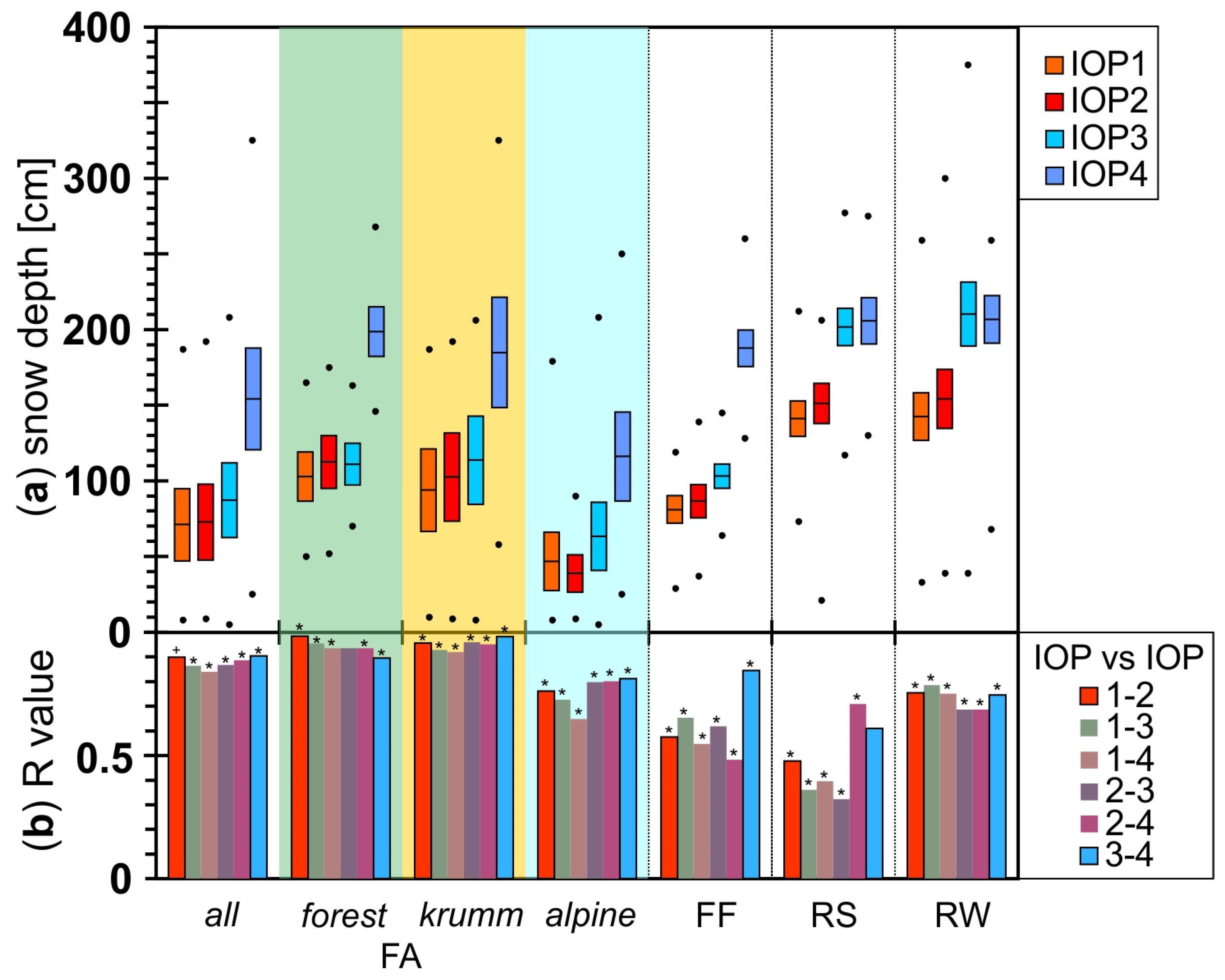
- The variability in snow depth is most temporally consistent in the forest (R approaching 1 over time), slightly less in the alpine (R is approximately 0.75), and least consistent in open terrain with mixed forests (R is approximately 0.6). Snow depth is more consistent intra-annually than inter-annually.
- (2)
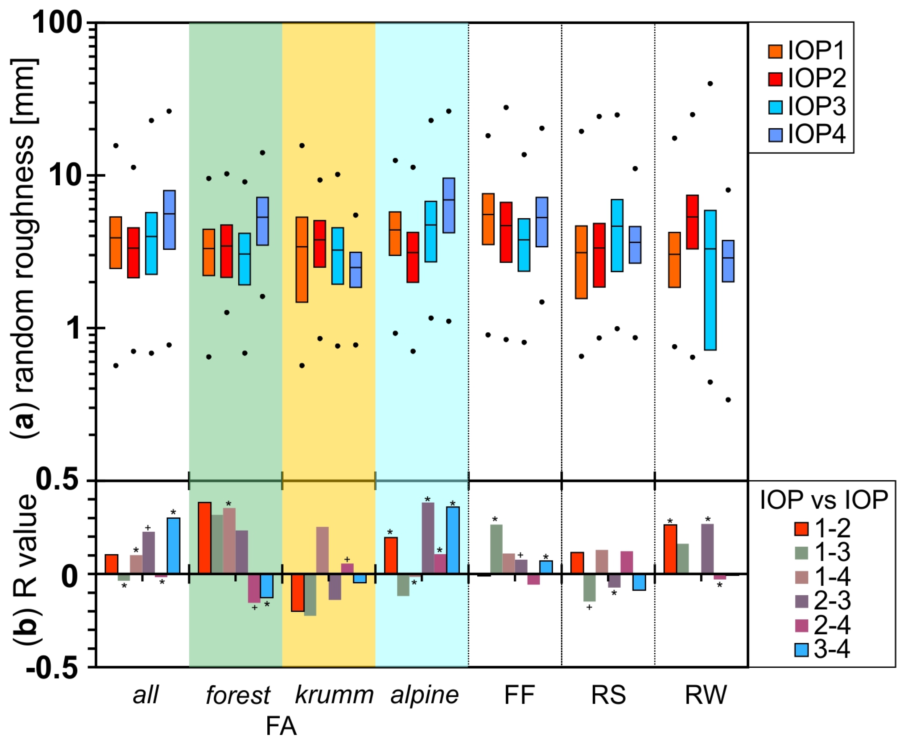
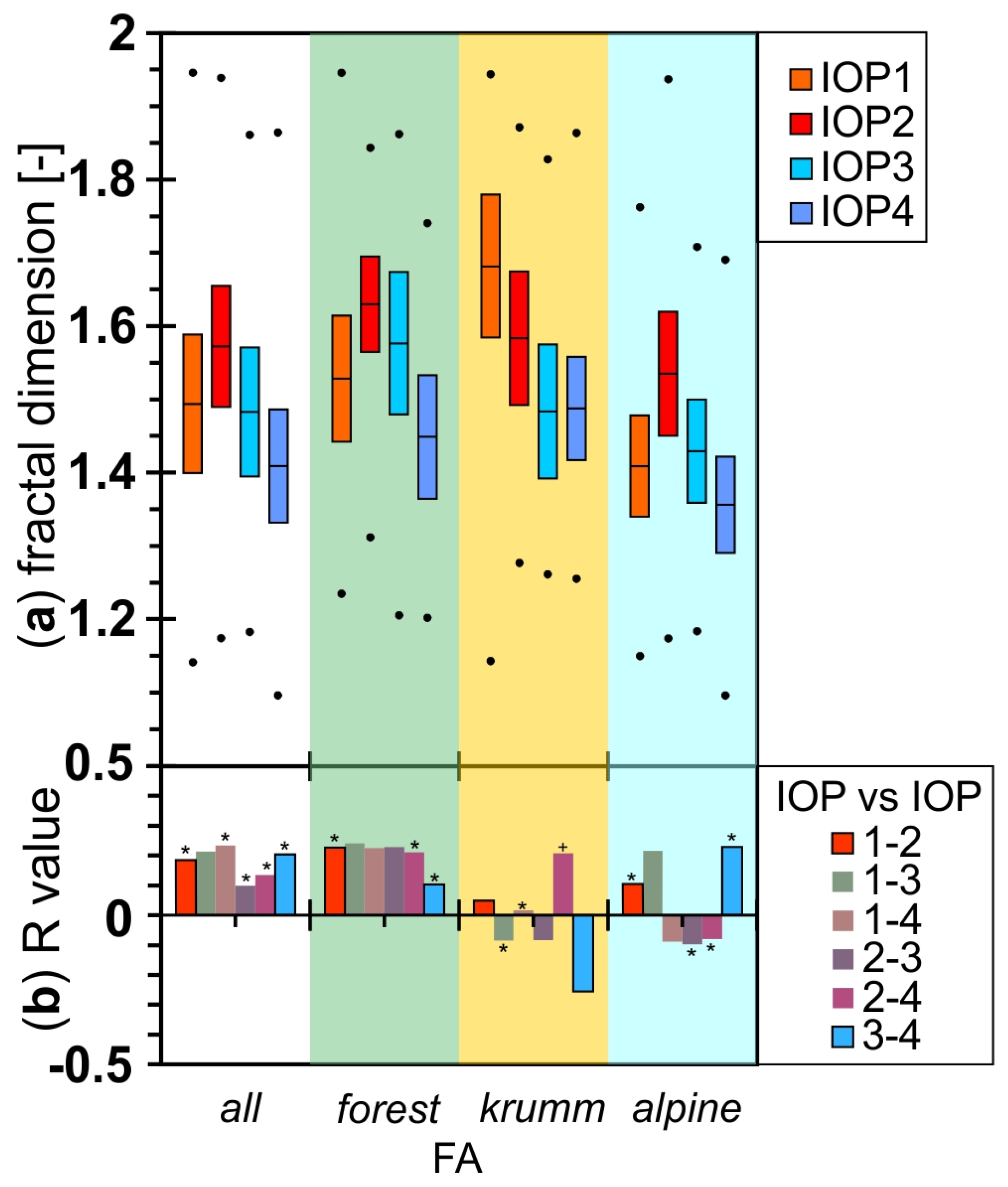
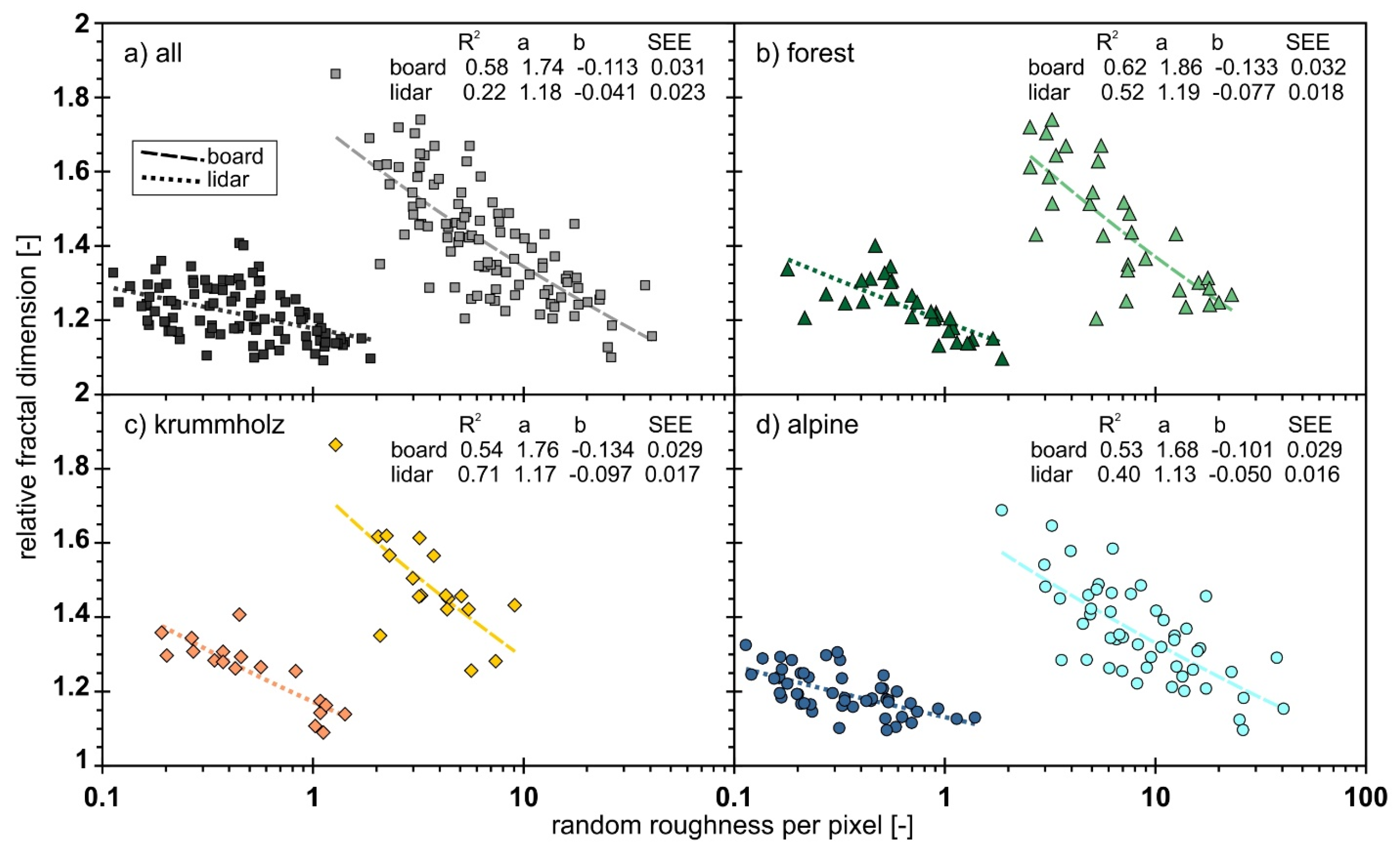
- Snow surface roughness, as defined by the random roughness, varies by up to 1.5 orders of magnitude over space. Mean random roughness values vary by a factor of 2 or 3 across the various study domains. This was observed for the boards and the lidar-derived snow surfaces. The fractal dimension value varies from 1.1 to 1.95 for the boards and by less than half for the lidar-derived snow surfaces (1.1 to 2.4).
- (3)
- Snow surface roughness from the boards is not temporally consistent; the maximum R-value for random roughness is 0.35, with most intra- and inter-annual comparisons being less than 0.2. Temporal consistency is less for the fractal dimension, with R being less than 0.2. Lidar data were only available for one time period, and thus the temporal variability was not assessed.
- (4)
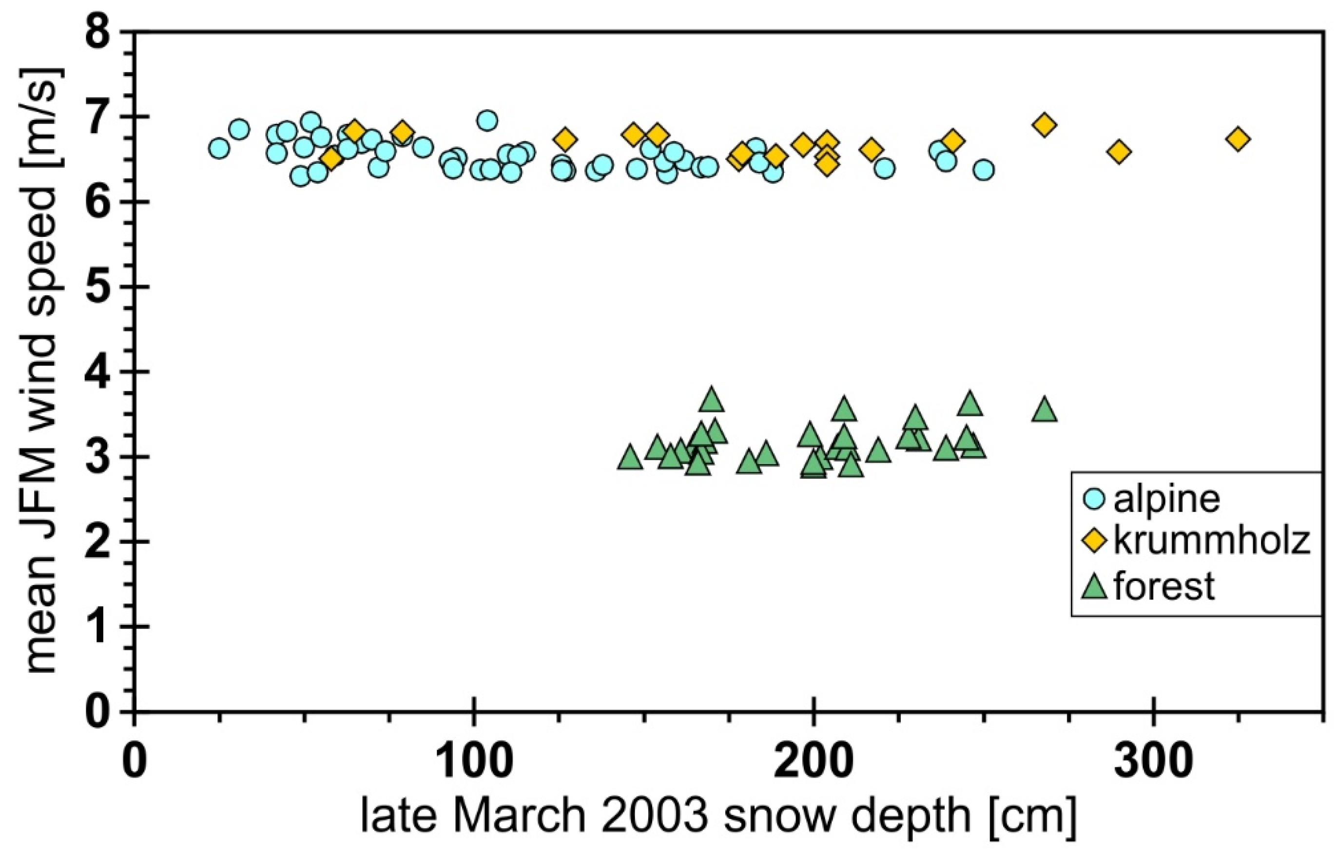
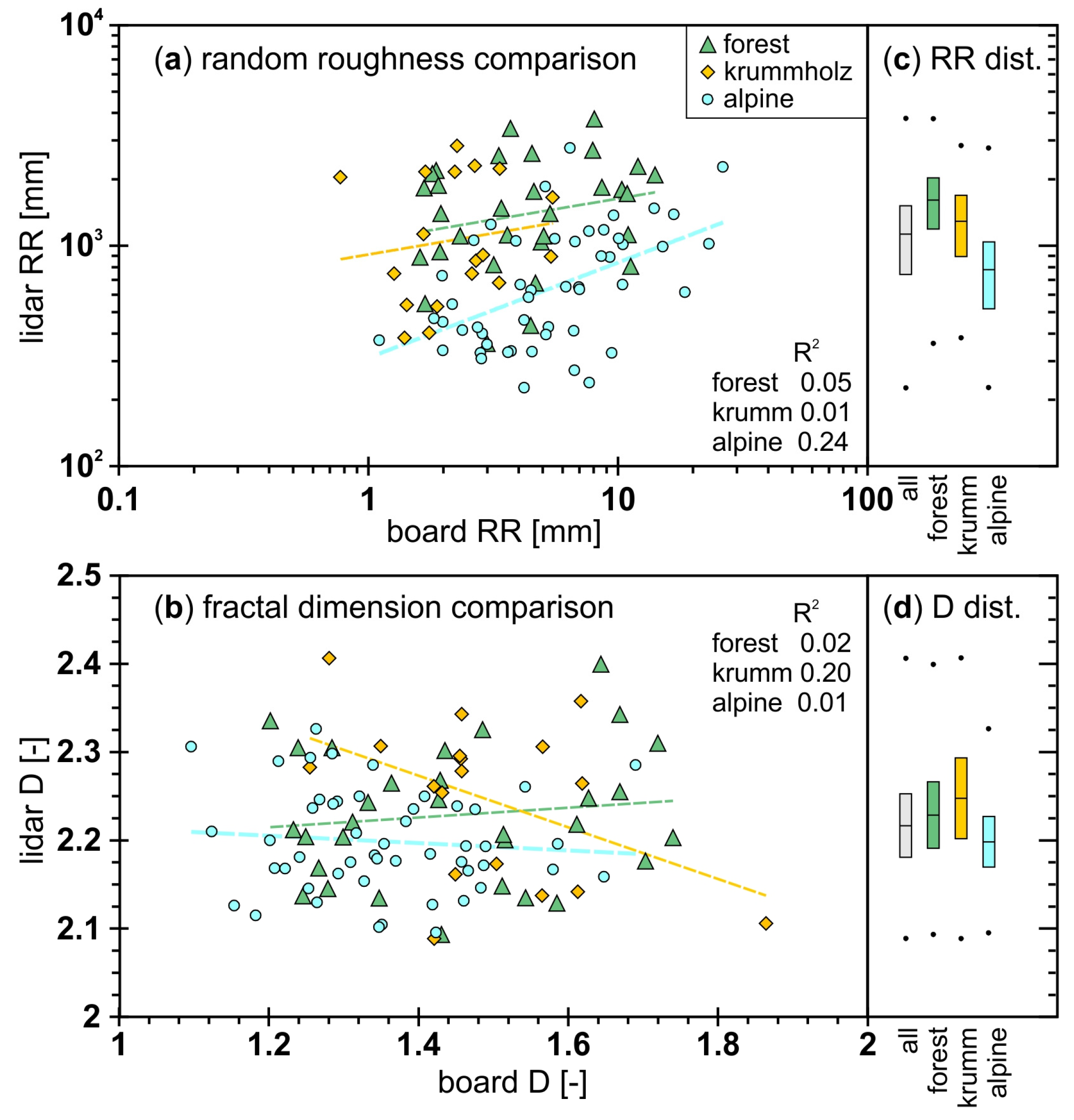
- Snow surface roughness is correlated with land cover characteristics. Alpine has a larger random roughness and is more organized (lower fractal dimension) than forest. The values for krummholz are between alpine and forest.
- (5)
- The two snow surface roughness metrics are not correlated across spatial scales, i.e., from the boards at millimeter resolution to the lidar data at meter resolution.
- (6)
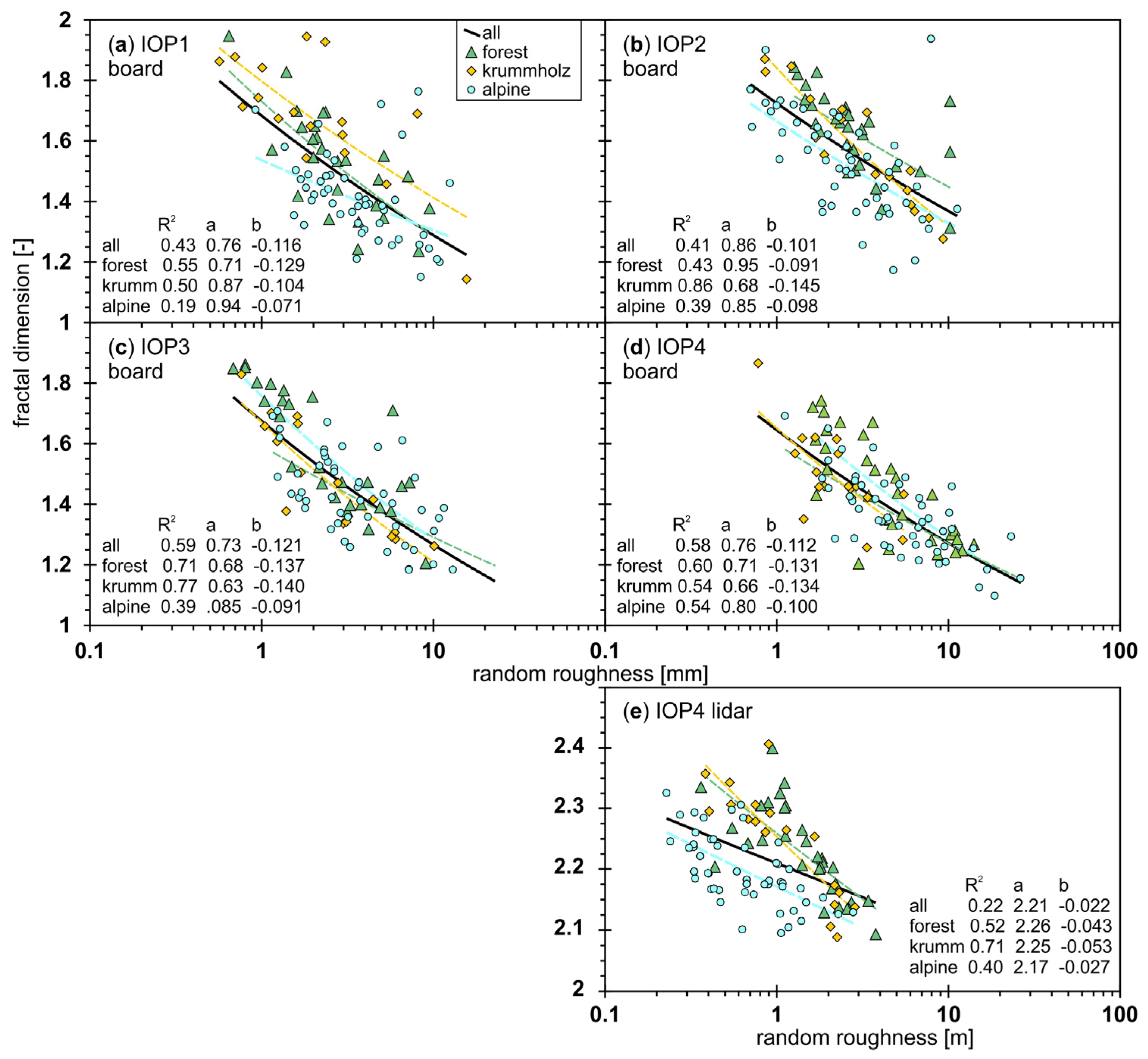
- The roughness metrics (i.e., RR and D) are well correlated, especially when separated by land cover. The correlation is more obvious when the dimension is removed from the roughness metrics.
Author Contributions
Funding
Data Availability Statement
Acknowledgments
Conflicts of Interest
Abbreviations
| CLPX | Cold Land Processes Experiment |
| D | fractal dimension |
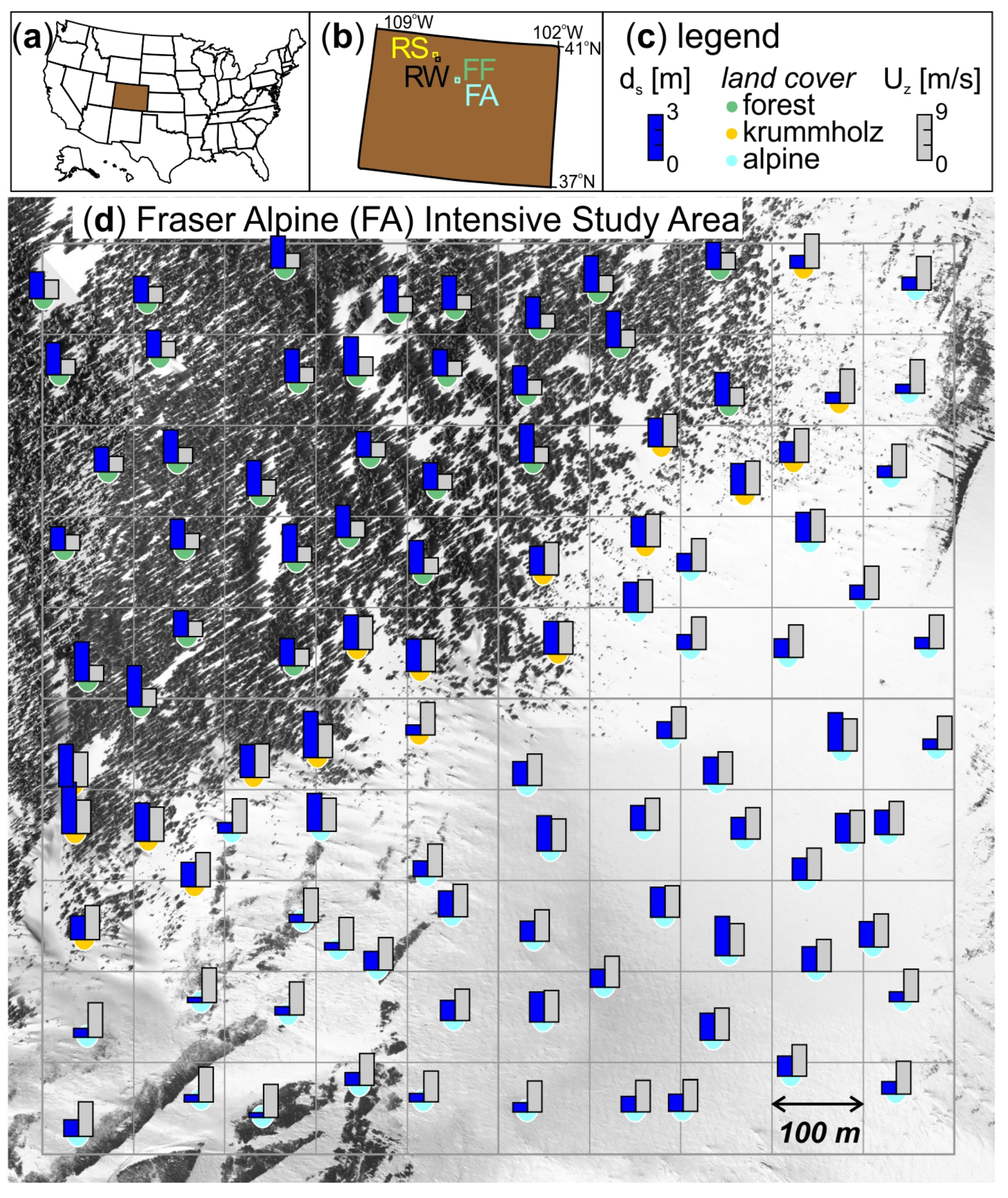
| FA | Fraser Alpine ISA |
| FF | Fool Creek ISA |
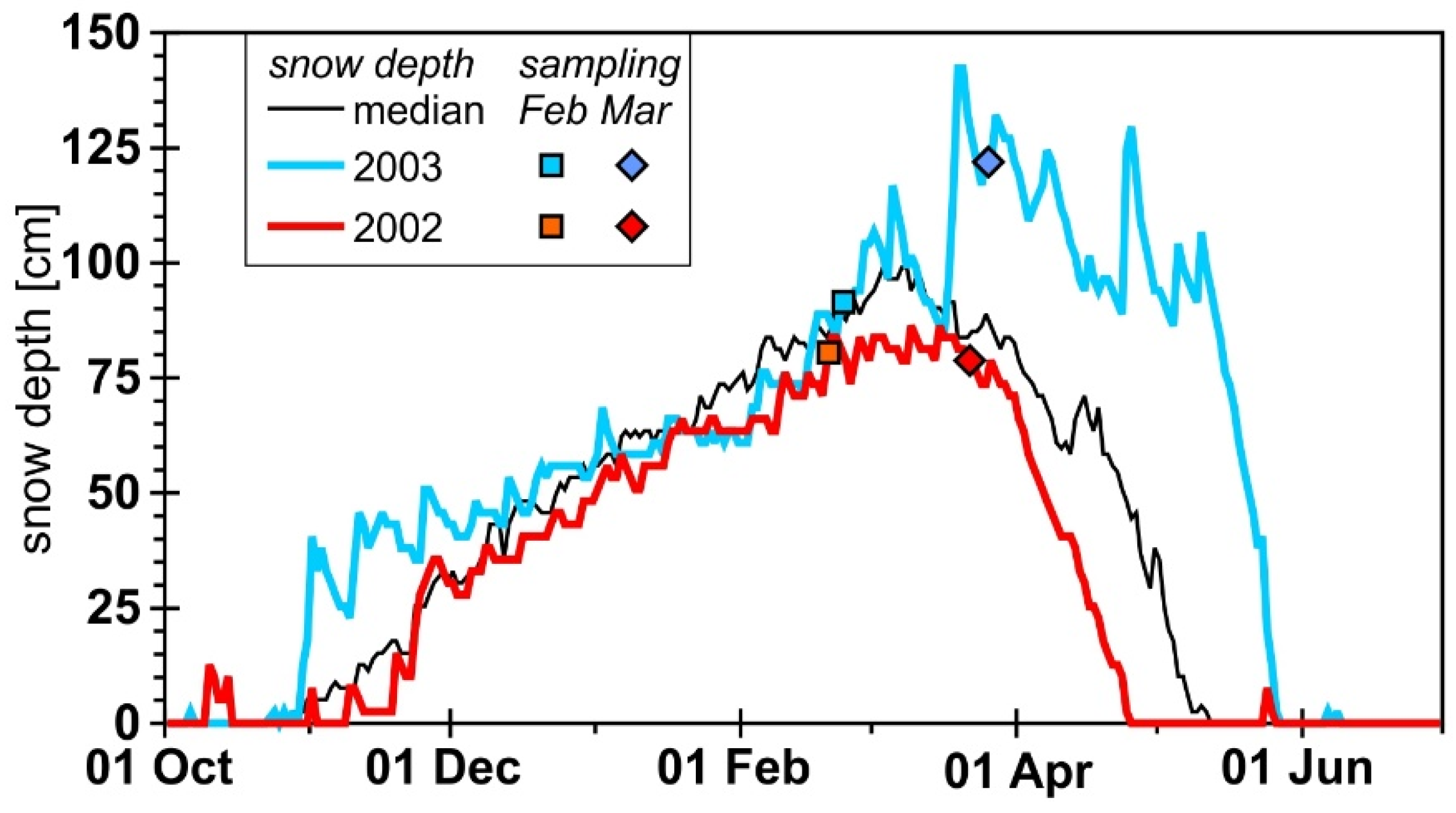
| IOP | Intensive Observation Period (IOP1 = February 2002, IOP2 = March 2002, IOP3 = February 2003, IOP4 = March 2003) |
| ISA | Intensive Study Area |
| NLDAS | North American Land Data Assimilation System |
| R | correlation coefficient (−1 to +1) |
| R2 | coefficient of determination (0 to 1) |
| RR | random roughness |
| RS | Rabbit Ears Spring Creek ISA |
| RW | Rabbit Ears Walton Creek ISA |
Appendix A. Fractal Analysis

References
- Oke, T.R. Boundary Layer Climates, 2nd ed.; Cambridge University Press: Cambridge, UK, 1987; ISBN 0-415-04319-0. [Google Scholar]
- Munro, D.S. Surface roughness and bulk heat transfer on a glacier: Comparison with eddy correlation. J. Glaciol. 1989, 35, 343–348. [Google Scholar] [CrossRef] [Green Version]
- Krinner, G.; Derksen, C.; Essery, R.; Flanner, M.; Hagemann, S.; Clark, M.; Hall, A.; Rott, H.; Brutel-Vuilmet, C.; Zhu, D.; et al. ESM-SnowMIP: Assessing snow models and quantifying snow-related climate feedbacks. Geosci. Model Dev. 2018, 11, 5027–5049. [Google Scholar] [CrossRef] [Green Version]
- Sexstone, G.A.; Clow, D.; Stannard, D.; Fassnacht, S.R. Comparison of methods for quantifying surface sublimation over seasonally snow-covered terrain. Hydrol. Process. 2016, 30, 3373–3389. [Google Scholar] [CrossRef]
- Marsh, C.B.; Pomeroy, J.W.; Spiteri, R.J.; Wheater, H.S. A finite volume blowing snow model for use with variable resolution meshes. Water Resour. Res. 2020, 56, e2019WR025307. [Google Scholar] [CrossRef]
- Sanow, J.E.; Fassnacht, S.R.; Kamin, D.J.; Sexstone, G.A.; Bauerle, W.L.; Oprea, I. Geometric Versus Anemometric Surface Roughness for a Shallow Accumulating Snowpack. Geosciences 2018, 8, 463. [Google Scholar] [CrossRef] [Green Version]
- Brock, B.; Willis, I.; Sharp, M. Measurement and parameterization of aerodynamic roughness length variations at Haut Glacier d’Arolla, Switzerland. J. Glaciol. 2006, 52, 281–297. [Google Scholar] [CrossRef] [Green Version]
- Fassnacht, S.R.; Williams, M.W.; Corrao, M.V. Changes in the surface roughness of snow from millimetre to metre scales. Ecol. Complex. 2009, 6, 221–229. [Google Scholar] [CrossRef]
- Fassnacht, S.R.; Toro Velasco, M.; Meiman, P.J.; Whitt, Z.C. The effect of aeolian deposition on the surface roughness of melting snow, Byers Peninsula, Antarctica. Hydrol. Process. 2010, 24, 2007–2013. [Google Scholar] [CrossRef]
- Suzuki, K.; Nakai, Y. Canopy snow influence on water and energy balances in a coniferous forest plantation in northern Japan. J. Hydrol. 2008, 352, 126–138. [Google Scholar] [CrossRef]
- Fassnacht, S.R.; Stednick, J.D.; Deems, J.S.; Corrao, M.V. Metrics for assessing snow surface roughness from digital imagery. Water Resour. Res. 2009, 45, W00D31. [Google Scholar] [CrossRef]
- Andreas, E.L. A relationship between the aerodynamic and physical roughness of winter sea ice. Q.J.R. Meteorol. Soc. 2011, 137, 1581–1588. [Google Scholar] [CrossRef]
- Fassnacht, S.R.; Oprea, I.; Borleske, G.; Kamin, D.J. Comparing snow surface roughness metrics with a geometric-based roughness length. In Proceedings of the AGU Hydrology Days Conference, Fort Collins CO, 24–26 March 2014; Ramirez, J.A., Ed.; Colorado State University: Fort Collins Colorado, CO, USA, 2014; Volume 34, pp. 44–52. [Google Scholar] [CrossRef]
- Smith, M. Roughness in the earth sciences. Earth-Sci. Rev. 2014, 136, 202–225. [Google Scholar] [CrossRef]
- Lettau, H. Note on aerodynamic roughness-parameter estimation on the basis of roughness-element description. J. Appl. Meteorol. 1969, 8, 828–832. [Google Scholar] [CrossRef]
- Kuipers, H. A reliefmeter for soil cultivation studies. Neth. J. Agric. Sci. 1957, 5, 255–267. [Google Scholar] [CrossRef]
- Deems, J.E.; Fassnacht, S.R.; Elder, K.J. Fractal Distribution of Snow Depth from Lidar Data. J. Hydrometeorol. 2006, 7, 285–297. [Google Scholar] [CrossRef]
- Elder, K.; Cline, D.; Liston, G.; Armstrong, R. NASA Cold Land Processes Experiment (CLPX 2002/03): Field Measurements of Snowpack Properties and Soil Moisture. J. Hydrometeorol. 2009, 10, 320–329. [Google Scholar] [CrossRef] [Green Version]
- Cline, D.; Yueh, S.; Chapman, B.; Stankov, B.; Gasiewski, A.; Masters, D.; Elder, K.; Kelly, R.; Painter, T.H.; Mahrt, L.; et al. NASA Cold Land Processes Experiment (CLPX 2002/03): Airborne remote sensing. J. Hydrometeorol. 2009, 10, 338–346. [Google Scholar] [CrossRef]
- Tedesche, M.E.; Fassnacht, S.R.; Meiman, P.J. Scales of Snow Depth Variability in High Elevation Rangeland Sagebrush. Front. Earth Sci. 2017, 11, 469–481. [Google Scholar] [CrossRef]
- Cline, D.; Armstrong, R.; Davis, R.; Elder, K.; Liston, G.E. CLPX-Ground: ISA Snow Pit Measurements, Version 2 [Data Set]; NASA National Snow and Ice Data Center Distributed Active Archive Center: Boulder, CO, USA, 2003; Available online: https://nsidc.org/data/nsidc-0176/versions/2 (accessed on 16 May 2023). [CrossRef]
- Miller, S. CLPX-Airborne: Infrared Orthophotography and Lidar Topographic Mapping, Version 1 [Data Set]; NASA National Snow and Ice Data Center Distributed Active Archive Center: Boulder, CO, USA, 2004; Available online: https://nsidc.org/data/nsidc-0157/versions/1 (accessed on 16 May 2023). [CrossRef]
- Sexstone, G.A.; Clow, D.W.; Fassnacht, S.R.; Liston, G.E.; Hiemstra, C.A.; Knowles, J.F.; Penn, C.A. Snow sublimation in mountain environments and its sensitivity to forest disturbance and climate warming. Water Resour. Res. 2018, 54, 1191–1211. [Google Scholar] [CrossRef]
- Sexstone, G.A.; Clow, D.W.; Penn, C.A. SnowModel Simulations and Supporting Observations for the North-Central Colorado Rocky Mountains during Water Years 2011 through 2015. U.S. Geological Survey Data Release 2018. Available online: https://www.usgs.gov/data/snowmodel-simulations-and-supporting-observations-north-central-colorado-rocky-mountains (accessed on 16 April 2023). [CrossRef]
- Cline, D.; Armstrong, R.; Davis, R.; Elder, K.; Liston, G.E. CLPX-Ground: ISA Snow Depth Transects and Related Measurements, Version 2 [Data Set]; NASA National Snow and Ice Data Center Distributed Active Archive Center: Boulder, CO, USA, 2003; Available online: https://nsidc.org/data/nsidc-0175/versions/2 (accessed on 16 May 2023). [CrossRef]
- Mitchell, K.E.; Lohmann, D.; Houser, P.R.; Wood, E.F.; Schaake, J.C.; Robock, A.; Cosgrove, B.A.; Sheffield, J.; Duan, Q.; Luo, L.; et al. The multi-institution North American Land Data Assimilation System (NLDAS): Utilizing multiple GCIP products and partners in a continental distributed hydrological modeling system. J. Geophys. Res. 2004, 109, D07S90. [Google Scholar] [CrossRef] [Green Version]
- Liston, G.E.; Elder, K. A Meteorological Distribution System for High-Resolution Terrestrial Modeling (MicroMet). J. Hydrometeor. 2006, 7, 217–234. [Google Scholar] [CrossRef] [Green Version]
- Liston, G.E.; Elder, K. A Distributed Snow-Evolution Modeling System (SnowModel). J. Hydrometeor. 2006, 7, 1259–1276. [Google Scholar] [CrossRef] [Green Version]
- Erickson, T.A.; Williams, M.W.; Winstral, A. Persistence of topographic controls on the spatial distribution of snow in rugged mountain terrain, Colorado, United States. Water Resour. Res. 2005, 41, W04014. [Google Scholar] [CrossRef] [Green Version]
- Deems, J.S.; Fassnacht, S.R.; Elder, K.J. Interannual consistency in fractal snow depth patterns at two Colorado mountain sites. J. Hydrometeorol. 2008, 9, 977–988. [Google Scholar] [CrossRef]
- Sturm, M.; Wagner, A.M. Using repeated patterns in snow distribution modeling: An Arctic example. Water Resour. Res. 2010, 46, W12549. [Google Scholar] [CrossRef] [Green Version]
- Mendoza, P.A.; Musselman, K.N.; Revuelto, J.; Deems, J.S.; López-Moreno, J.I.; McPhee, J. Interannual and seasonal variability of snow depth scaling behavior in a subalpine catchment. Water Resour. Res. 2020, 55, e2020WR027343. [Google Scholar] [CrossRef]
- Revuelto, J.; Alonso-González, E.; López-Moreno, J. Generation of daily high-spatial resolution snow depth maps from in-situ measurement and time-lapse photographs. Cuad. Investig. Geográfica/Geogr. Res. Lett. 2020, 46, 59–79. [Google Scholar] [CrossRef] [Green Version]
- Sturm, M.; Holmgren, J. An automatic snow depth probe for field validation campaigns. Water Resour. Res. 2018, 54, 9695–9701. [Google Scholar] [CrossRef]
- Fassnacht, S.R.; Brown, K.S.; Blumberg, E.J.; López Moreno, J.I.; Covino, T.P.; Kappas, M.; Huang, Y.; Leone, V.; Kashipazha, A.H. Distribution of Snow Depth Variability. Front. Earth Sci. 2018, 12, 683–692. [Google Scholar] [CrossRef]
- Fassnacht, S.R. A Call for More Snow Sampling. Geosciences 2021, 11, 435. [Google Scholar] [CrossRef]
- Deems, J.S.; Painter, T.H.; Finnegan, D.C. Lidar measurement of snow depth: A review. J. Glaciol. 2013, 59, 467–479. [Google Scholar] [CrossRef] [Green Version]
- Nolan, M.; Larsen, C.; Sturm, M. Mapping snow depth from manned aircraft on landscape scales at centimeter resolution using structure-from-motion photogrammetry. Cryosphere 2015, 9, 1445–1463. [Google Scholar] [CrossRef] [Green Version]
- Pflug, J.M.; Lundquist, J.D. Inferring distributed snow depth by leveraging snow pattern repeatability: Investigation using 47 lidar observations in the Tuolumne watershed, Sierra Nevada, California. Water Resour. Res. 2020, 56, e2020WR027243. [Google Scholar] [CrossRef]
- Manes, C.; Guala, M.; Löwe, H.; Bartlett, S.; Egli, L.; Lehning, M. Statistical properties of fresh snow roughness. Water Resour. Res. 2008, 44, W11407. [Google Scholar] [CrossRef] [Green Version]
- Gromke, C.; Manes, C.; Walter, B.; Lehning, M.; Guala, M. Aerodynamic Roughness Length of Fresh Snow. Bound. -Layer Meteorol. 2011, 141, 21–34. [Google Scholar] [CrossRef] [Green Version]
- Trujillo, E.; Ramírez, J.A.; Elder, K.J. Topographic, meteorologic, and canopy controls on the scaling characteristics of the spatial distribution of snow depth fields. Water Resour. Res. 2007, 43, W07409. [Google Scholar] [CrossRef]
- Sturm, M.; Holmgren, J.; McFadden, J.P.; Liston, G.E.; Chapin, F.S., III; Racine, C.H. Snow–Shrub Interactions in Arctic Tundra: A Hypothesis with Climatic Implications. J. Clim. 2001, 14, 336–344. [Google Scholar] [CrossRef]
- Hiemstra, C.A.; Liston, G.E.; Reiners, W.A. Snow Redistribution by Wind and Interactions with Vegetation at Upper Treeline in the Medicine Bow Mountains, Wyoming, USA. Arct. Antarct. Alp. Res. 2002, 34, 262–273. [Google Scholar] [CrossRef]
- Ewing, P.J.; Fassnacht, S.R. From the tree to the forest: The influence of a sparse canopy on stand scale snow water equivalent. In Proceedings of the Eastern Snow Conference, St. John’s, NL, Canada, 29 May–1 June 2007; Volume 64, pp. 149–163. [Google Scholar]
- Suzuki, K.; Ohta, T.; Kojima, A.; Hashimoto, T. Variations in snowmelt energy and energy balance characteristics with larch forest density on Mt Iwate, Japan: Observations and energy balance analyses. Hydrol. Process. 1999, 13, 2675–2688. [Google Scholar] [CrossRef]
- López-Moreno, J.I.; Revuelto, J.; Fassnacht, S.R.; Azorín-Molina, C.; Vicente-Serrano, S.M.; Morán-Tejeda, E.; Sexstone, G.A. Snowpack variability across various spatio-temporal resolutions. Hydrol. Process. 2015, 29, 1213–1224. [Google Scholar] [CrossRef]
- López-Moreno, J.I.; Revuelto-Benedí, J.; Alonso-González, E.; Sanmiguel-Vallelado, A.; Fassnacht, S.R.; Deems, J.E.; Morán-Tejeda, E. Using Very Long-range Terrestrial Laser Scanner to Analyse the Temporal Consistency of the Snowpack Distribution in a High Mountain Environment. J. Mt. Sci. 2017, 14, 823–842. [Google Scholar] [CrossRef]
- Revuelto, J.; Alonso-Gonzalez, E.; Vidaller-Gayan, I.; Lacroix, E.; Izagirre, E.; Rodríguez-Lopez, G.; Ĺopez-Moreno, J.I. Intercomparison of UAV platforms for mapping snow depth distribution in complex alpine terrain. Cold Reg. Sci. Technol. 2021, 190, 103344. [Google Scholar] [CrossRef]
- Harder, P.; Pomeroy, J.W.; Helgason, W.D. Improving sub-canopy snow depth mapping with unmanned aerial vehicles: Lidar versus structure-from-motion techniques. Cryosphere 2020, 14, 1919–1935. [Google Scholar] [CrossRef]
- Nelson, P. Evaluation of Handheld Apple iPad LiDAR for Measurements of Topography and Geomorphic Change. In Proceedings of the American Geophysical Union Fall Meeting, New Orleans, LA, USA, 13–17 December 2021. [Google Scholar]
- Liu, J.; Chen, R.; Ma, S.; Guo, S.; Han, C.; Ding, Y. Quantifying the aerodynamic roughness length of snow surfaces with time-lapse structure-from-motion. J. Geophys. Res. Atmos. 2023, 128, e2022JD037032. [Google Scholar] [CrossRef]
- Sanow, J.E.; Fassnacht, S.R.; Suzuki, K. Inclusion of a Site Specific, Variable Aerodynamic Roughness Length (z0) in the SNOWPACK Model. In Proceedings of the ISAR-7 Seventh International Symposium on Arctic Research, Tachikawa, Japan, 6–10 March 2023; (abstract R5-S8-O02). [Google Scholar]
- Hultstrand, D.M.; Fassnacht, S.R. The Sensitivity of Snowpack Sublimation Estimates to Instrument and Measurement Uncertainty Perturbed in a Monte Carlo Framework. Front. Earth Sci. 2018, 12, 728–738. [Google Scholar] [CrossRef]
- Chapin, H.; Chapin, S. Cat’s in the Cradle. In Chapter 1: Verities & Balderdash; Elektra Entertainment: Los Angeles, CA, USA, 1974. [Google Scholar]


Disclaimer/Publisher’s Note: The statements, opinions and data contained in all publications are solely those of the individual author(s) and contributor(s) and not of MDPI and/or the editor(s). MDPI and/or the editor(s) disclaim responsibility for any injury to people or property resulting from any ideas, methods, instructions or products referred to in the content. |
© 2023 by the authors. Licensee MDPI, Basel, Switzerland. This article is an open access article distributed under the terms and conditions of the Creative Commons Attribution (CC BY) license (https://creativecommons.org/licenses/by/4.0/).
Share and Cite
Fassnacht, S.R.; Suzuki, K.; Sanow, J.E.; Sexstone, G.A.; Pfohl, A.K.D.; Tedesche, M.E.; Simms, B.M.; Thomas, E.S. Snow Surface Roughness across Spatio-Temporal Scales. Water 2023, 15, 2196. https://doi.org/10.3390/w15122196
Fassnacht SR, Suzuki K, Sanow JE, Sexstone GA, Pfohl AKD, Tedesche ME, Simms BM, Thomas ES. Snow Surface Roughness across Spatio-Temporal Scales. Water. 2023; 15(12):2196. https://doi.org/10.3390/w15122196
Chicago/Turabian StyleFassnacht, Steven R., Kazuyoshi Suzuki, Jessica E. Sanow, Graham A. Sexstone, Anna K. D. Pfohl, Molly E. Tedesche, Bradley M. Simms, and Eric S. Thomas. 2023. "Snow Surface Roughness across Spatio-Temporal Scales" Water 15, no. 12: 2196. https://doi.org/10.3390/w15122196