Article

Hydrological Dynamics of the Pantanal, a Large Tropical Floodplain in Brazil, Revealed by Analysis of Sentinel-2 Satellite Imagery

by
Edelin Jean Milien
1,*,
Gustavo Manzon Nunes
2,
Girard Pierre
1,3,
Stephen K. Hamilton
4 and
Catia Núnes Da Cunha
1,5,*
1
Graduate Program in Ecology and Biodiversity Conservation, Institute of Biosciences, Federal University of Mato Grosso, Av. Fernando Correa da Costa, 2367, Cuiabá 78060-900, MT, Brazil
2
Graduate Program in Forest Engineering and Postgraduate Program in Forestry and Environmental Sciences, Faculty of Forestry Engineering, Federal University of Mato Grosso, Av. Fernando Correa da Costa, 2367, Cuiabá 78060-900, MT, Brazil
3
Pantanal Research Center (CPP), Av. Fernando Correa da Costa, 2367, Cuiabá 78060-900, MT, Brazil
4
Cary Institute of Ecosystem Studies, Michigan State University, 426, Auditorium Road, East Lansing, MI 48824, USA
5
Institute for Science and Technology of Wetlands (INCT-INAU), Av. Fernando Correa da Costa, 2367, Cuiabá 78060-900, MT, Brazil
*
Authors to whom correspondence should be addressed.
Water 2023, 15(12), 2180; https://doi.org/10.3390/w15122180
Submission received: 28 March 2023 / Revised: 2 June 2023 / Accepted: 7 June 2023 / Published: 9 June 2023
(This article belongs to the Topic Remote Sensing in Water Resources Management Models)

Abstract

:
Extensive tropical floodplain wetlands, such as the Brazilian Pantanal, are complex ecosystems composed of mosaics of permanently and seasonally flooded habitats and are increasingly threatened by land use and climate change. Spatial and interannual variability in the seasonal flood pulse is a fundamental ecological driver in these ecosystems. This study analyzes optical imagery from the Sentinel-2 satellite to determine the extent and seasonal patterns of inundation over five years in the northern Pantanal, a Ramsar site renowned for its wildlife. The study site is bordered by the Cuiabá and São Lourenço rivers, each with distinct flow regimes. Inundation patterns were revealed with a combination of water indices, supervised classification of land cover, and a digital elevation model. Total extent of flooding was underestimated by the optical imagery, but open water bodies were readily delineated with the land cover classification.

1. Introduction

Wetlands, which are among the most productive environments in the world [1], play a significant role in the water cycle [2] and are recognized as biodiversity hotspots, providing ecosystem services, such as regulation of the hydrological cycle, flood control, and improvement and maintenance of water quality, among others [3]. In extensive floodplain wetlands, spatial and interannual variability in the seasonal flood pulse is a fundamental ecological driver. Understanding the complex hydrology of floodplain wetlands is thus fundamental to the sustainable management of these environments [4]. Remote sensing of flood extent is also needed to understand and mitigate flood hazards [5,6]
The Pantanal, located mostly in Brazil, is one of the world’s largest floodplain wetlands and is listed as a World Heritage Site and as a biosphere reserve. Most of the Pantanal is subject to seasonal inundation driven by a variable combination of riverine overflow and delayed drainage of local rainfall [7]. Seasonal alternation between flooding and drying, often including fire during the dry season [8], determines the biodiversity and ecology of the floodplain environments, as conceptualized by the flood pulse concept [9]. The degree of seasonal hydrological connectivity between rivers and their floodplains varies spatially, resulting in some floodplain lands inundated primarily by river water and others flooded by local rainwater [10,11], corresponding with differences in the extent, duration, and depth of inundation as well as the supply of sediments and nutrients by flood waters (Fantin-Cruz et al., 2011). The ecological structure and function, including biogeochemical processes, of the Pantanal floodplains are therefore closely linked to hydrology [12,13].
Satellite remote sensing has increasingly been employed to study the hydrology [14] and ecology of extensive floodplain wetlands [15]. Vegetated floodplains are particularly challenging environments for remote sensing of surface water because tree and shrub canopies and emergent and floating herbaceous plants can partially or entirely obscure the water surface to a degree that varies with water depth and seasonal plant growth and senescence. In addition, the turbidity of surface waters in floodplains is typically extremely variable, ranging from rich in suspended sediments to dominance by phytoplankton to relatively clear depending on a water body’s connectivity with the river, water sources, sedimentation and sediment resuspension, and flushing rates. Microwave remote sensing can better detect water amongst vegetation, and radar altimetry can estimate the elevation of the water surface, but optical satellite observations offer greater temporal coverage, and image processing of optical data can reveal spectral features associated with different vegetation forms and water characteristics as well as open water surfaces at greater spatial resolution [16]. Additionally, compared with microwave remote sensing, optical remote-sensing-data availability and spatial data-processing techniques are more readily available to non-specialists [17,18].
In the Pantanal, studies have employed both microwave and optical sensor systems. Satellite observations of passive microwave emission were analyzed to provide a coarse-scale (~25 km) view of inundation patterns at monthly resolution across the entire Pantanal [19], and subsequent studies have incorporated data from similar sensors to estimate inundation patterns in floodplain wetlands across the tropics [20]. Dettmering [21] used ENVISAT radar altimetry to derive water level time series that showed seasonal variations of up to 1.5 m with maximum water levels between January and June, although some regions of the Pantanal showed water level variations of less than a few decimeters, which could not be quantified by the method. Evans [22] used L-band ALOS/PALSAR and C-band RADARSAT-2 synthetic aperture radar data to map land cover and seasonal inundation throughout the Brazilian Pantanal. Two studies have determined seasonal and interannual variation in the extent of inundation in the Brazilian Pantanal with MODIS optical satellite imagery [23,24].
The present study analyzes inundation and land cover in a large nature reserve in the northern Pantanal using optical imagery from the Sentinel-2 satellite, which provides superior spatial, temporal, and spectral resolution compared to the Landsat and MODIS sensor systems that have been used in past studies. Floodplain geomorphology and open water bodies were revealed with a combination of water indices, supervised classification of land cover, and a digital elevation model. Results for the open water area were comparable, but some differences are discussed. This information will be useful for the management and restoration of this reserve and similar areas in the Pantanal, and our approach can be applied in similar tropical floodplains.

2. Material and Methods

Study Site

The study site is a private reserve covering 108,095.3 ha in the northern Pantanal, situated between the Cuiabá and São Lourenço rivers (Figure 1). The reserve is known as SESC Pantanal and is owned by the National Trade Service [25]. As part of Brazil’s Reserva Particular do Patrimônio Natural (Private Reserve of National Patrimony) system, the lands are managed for conservation and environmental education. The SESC Pantanal reserve is designated as a Ramsar site in recognition of its biodiversity (Cunha et al., 2019).
Seemingly minor variations in land surface elevation determine water flow and inundation patterns in floodplains, such as the Pantanal. Topographic variation in the Pantanal reflects Pleistocene and Holocene sediment depositional processes [24,26]. Assine [27] has shown that the depositional systems of the Pantanal are composed by fluvial megafans, fluvial plains, and lacustrine systems. Geomorphology and hydrology determine the vegetation, which has been classified throughout the Pantanal to the level of macrohabitats [28].
According to Pupim [13], the study site spans parts of the alluvial megafans of the Cuiabá and São Lourenço rivers, with fluvial plains, fluviolacustrine plains, and relatively level, seasonally or permanently flooded areas that have sandy soils and are poorly connected to the drainage network, yet susceptible to inundation by the largest floods whose dynamics are controlled by riverine overflow and backwater effects. Based on hydro-sedimentological characteristics, the site can be divided into two geomorphological units, the modern depositional lobes and the Cuiabá River anastomosed active floodplains. The modern depositional lobes are formed by a distributary network of channels and levees within the São Lourenço megafan. A significant avulsion event in the lower Holocene abruptly changed the course of the São Lourenço River [13], which caused the abandonment of part of the meander belt and led to the creation of modern floodplain lakes that are still present today. The anastomosing floodplain flow paths are subject to flooding by the Cuiabá River and by significant water input from neighboring drainage systems, with a fluvial belt built by multiple branching channels.
In the northern Pantanal, the rainy season extends from October to March, with the most intense rains usually from January to March. The dry season extends from April to September, and the driest months are from July to September. The discharge peaks in the Cuiabá and São Lourenço rivers are generally reached between February and April, with lowest discharge recorded between August and October [11] Floodplain inundation peaks toward the latter part of the wet season.

3. Methods

The methodological steps are summarized in Figure 2.

3.1. Data Sources

3.1.1. Hydrological Data

We used data from the National Water Agency (ANA) that were acquired from the agency’s website (https://www.snirh.gov.br/hidroweb/serieshistoricas) (accessed on 23 February 2021). Since our study area is bounded by both the Cuiabá and the São Lourenço rivers, it was necessary to download fluviometric data for both major rivers. The two stations were Porto Cercado on the Cuiabá River (station code 66340000) and Acima do Córrego Grande on the São Lourenço River (station code 66460000). Hydrographs of mean monthly discharge indicated the relative timing and intensity of floodplain inundation by the two rivers.

3.1.2. Water Index and Supervised Classification Data
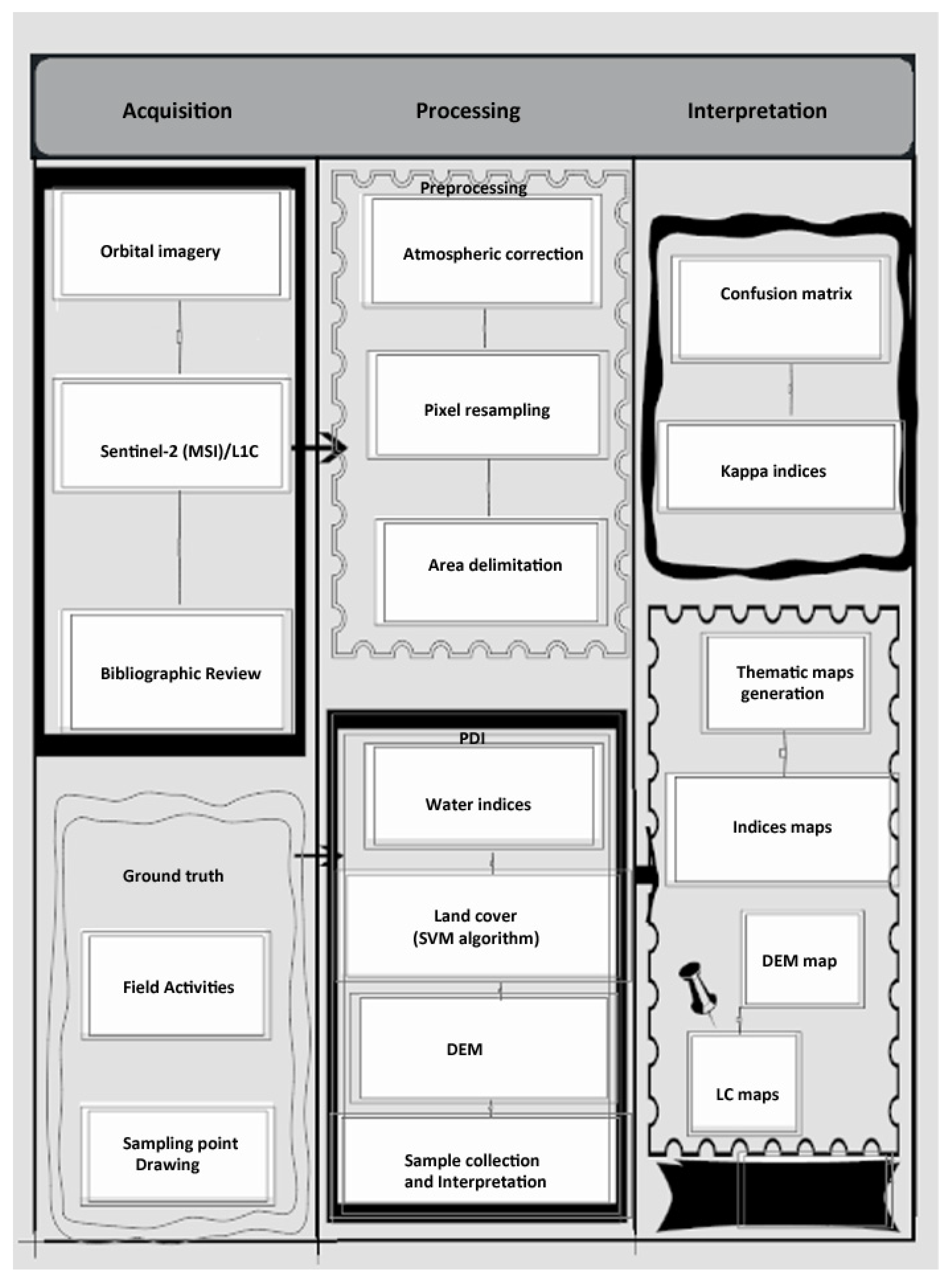
We analyzed optical data from the Sentinel-2 satellite to determine inundation patterns and land cover. Sentinel-2 is a wide-swath, high-resolution, multi-spectral imaging mission launched in 2014 and supported by the European Space Agency. Twin satellites fly in the same orbit but phased at 180° to provide a revisit frequency of five days at the Equator.
Scenes were chosen using the river hydrographs as indicators of inundation over the period from 2015 to 2020. Since the highest water levels did not occur simultaneously throughout the study area, dates of maximum inundation were estimated separately for the two rivers (Cuiabá and São Lourenço) based on their hydrographs. The image product downloaded from https://earthexplorer.usgs.gov (accessed on 26 July 2021) was the Top-Of-Atmosphere Level-1C, which has 10–60 m spatial resolution and 10-day temporal resolution and is available without cost [29].

3.2. Preprocessing

3.2.1. Atmospheric Correction

Atmospheric corrections were performed to reduce the scattering, absorption, and refraction of electromagnetic energy that affect the reflectance from the land surface captured by the sensor. Atmospheric correction also reduces the possibility of detecting small objects within a scene or differentiating between objects of similar signal intensity [30]. Atmospheric correction of satellite images serves not only to minimize atmospheric effects on the radiance of a scene (Neto et al., 2011) but is also necessary to calculate water indices computed from two or more spectral bands since the bands are affected differently by atmospheric scattering.
For this study, the TOA (top of atmosphere) was corrected to BOA (bottom of atmosphere) using the SNAP program (Sen2Cor processor) available from the ESA [31]. The algorithm is based on a set of 24 lookup tables that cover most of the Earth’s atmospheric conditions [32]. To perform the correction, the application consists of a set of command-line-oriented modules written in Python programming language, which must be incorporated into the tools (toolboxes) of the SNAP software provided by the European Space Agency for handling and processing Sentinel images [32].

3.2.2. Resampling Bands

After atmospheric correction of the Sentinel-2 satellite images, the SNAP program was used to resample the bands. Since the Sentinel-2 product has 12 spectral bands with different spatial resolutions, it was necessary to resample so that all bands needed for the work were at the same spatial resolution. The modified normalized water index (MNDWI), which we used to detect water bodies, requires the use of MSI band 11 (SWIR), which has a spatial resolution of 20 m, and band 3 (green), which has a spatial resolution of 10 m.

3.3. Digital Processing Image (DPI)

3.3.1. Spectral Water Index

The normalized difference water index (NDWI) was developed to identify open water in digital remote-sensing images [33]. NDWI uses reflected infrared radiation and visible green light to highlight the presence of open water against a background of soil and terrestrial vegetation features. The NDWI was calculated as band math in ENVI software using Equation (1):
NDWI   = ( Green NIR ) ( Green + NIR )
where green is the BOA reflectance of the B3 band (green band), and NIR is the BOA reflectance of the B8 band (NIR band) of the Sentinel-2 MSI image.
The MNDWI (modified NDWI) was designed to minimize the main limitation of NDWI, which is the inefficiency of suppressing the noise coming from the characteristics of the built-up areas [34]. Thus, the MNDWI was developed considering that a water body presents higher absorption in the SWIR (shortwave infrared) band compared to the NIR band, unlike built-up areas. We considered positive values (>0.0) of both indices to indicate open water [33,35]. The MNDWI was calculated as band math in ENVI software using Equation (2):
MNDWI   = ( Green SWIR 1 ) ( Green + SWIR 1 )

3.3.2. Supervised Classification

The images were analyzed by supervised classification through the support vector machine (SVM) algorithms processed in the ENVI software. The analyses performed were processing, image classification, and evaluation of the algorithms applied. In the processing phase, the images were prepared using a radial basis function as a kernel to support vector classification.
From the INPE (National Institute of Space Research of Brazil) map of vegetation and land cover use proposed by [36], six thematic classes of land cover were defined: shrub; dry forest/monodominant forest; water body; flooded fields; dry fields; and exposed soil. We identified 5909 training sample pixels for each class.

3.3.3. Error Matrix and Kappa Index

Independent observations representing the mapped land cover classes served for post-classification validation. According to Jensen [37], for validation in situations where the coverage area corresponds to up to 4050 km2, at least 50 samples are needed for each mapped class. Since our study area of 88 km2 is much smaller than that, 96 observations were recorded in the field with GPS coordinates, and 250 samples were collected using satellite imagery available in the Google Earth Pro software.
Classification accuracy was assessed by comparing the land cover classification with the field and Google Earth observations. False positives (errors of commission) and the false negatives (errors of omission) were evaluated. Accuracy varied by land cover class and may thus be higher or lower at a given pixel. The confusion matrix, accuracy evaluation, and Kappa correlation coefficient for the land cover classification, following the concepts of [38], were generated for two periods: (1) May 2017: accuracy: 98.92%, Kappa coefficient: 0.97; and (2) September–May 2017: accuracy: 97.89%, Kappa coefficient: 0.97.

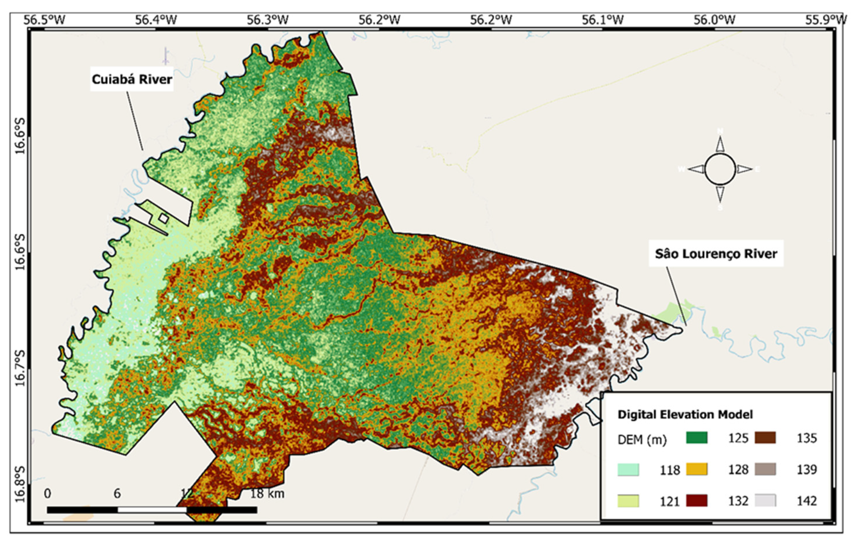
3.4. Digital Elevation Model

Since elevation of the floodplain land surface determines inundation by the rivers, a digital elevation model was created for comparison with river stage data. We used ALOS PALSAR satellite observations to map the topographic surface at 12.5-m spatial resolution. We downloaded the radiometrically terrain-corrected product from the Alaska Satellite Facility https://asf.alaska.edu/data-sets/sar-data-sets/alos-palsar/ (accessed on 29 August 2021). The satellite was launched in January 2006 by JAXA (Japan Aerospace Exploration Agency).

3.5. Data Analysis

After data acquisition and processing, we analyzed the spatial variability and temporal dynamics of water along the study area. Using geoprocessing techniques, classes pixels were extracted for the study area in a spatial cutout. With those data, we obtained estimates of open water over time inside all the reserve for analysis. We then compared estimates of water and other classes inside and the reserve and conducted statistical analysis to assess their statistical significance of the differences. For purposes of inferential testing, we first applied a normality test using the Shapiro model, considered the most powerful normality test, followed by the Anderson–Darling test [39]. We then selected our statistical tests based on the results of the normality tests. Parametric statistical analysis assumes a normal distribution in data. But if the normality assumption is violated, parametric tests may not be reliable or valid for drawing conclusions [39]. The normality tests verified that the data distributions were non-normal; thus, parametric tests would not be appropriate. We therefore employed the Kruskal–Wallis test to assess the statistical significance of differences between water and others rates inside the study area over time.

4. Results

4.1. River Discharge

Mean monthly discharge of the Cuiabá River from 2015 to 2020 is shown in Figure 3. The season of high discharge was similar for the two rivers, although they reached their maximum discharge in different years (2017 for the Cuiabá River and 2018 for the São Lourenço River). The Cuiabá River reached a consistently low minimum annual discharge every year, whereas the São Lourenço River was more variable from year to year in its lowest discharge, and throughout the year, month-to-month changes in its discharge were less gradual. The lowest discharges for both rivers occurred in 2020. Following the annual minimum discharge, the São Lourenço River tended to rise in discharge earlier than the Cuiabá.
Overbank flow from these two rivers via distributary channels inundated parts of the study site between November and April. The central part of the site tends to be flooded by local rain due to its elevation and distance from the rivers as well as the low permeability of the subsurface soil horizons.
Based on the observations in Figure 3, the most extensive discharge of the study site likely occurred in April 2017, driven by overbank flow from the Cuiabá River. The highest discharge measured in the São Lourenço River was April 2018 and occurred during the rainy season, while the lowest recorded discharge coincided with the dry season.

4.2. Hypsometric Mapping

A hypsometric map was made from the DEM to delineate the lower lying areas that are most readily subject to river inundation (i.e., the active floodplain that floods frequently) from the relatively inactive paleo-floodplain (Figure 4). This map shows that the lowest points in the area are concentrated in the Cuiabá River floodplain and range in elevation between 118 and 121 m (Figure 4). The DEM shows the water bodies in the floodplain that are subject to seasonal inundation by the Cuiabá River through natural side channels as well as some artificial breaks through levees opened by ranchers since the 1980s.
The active floodplain was calculated as 26,034 hectares using a buffer of 10 km with the Cuiabá River line in ArcGIS Pro software and considering that the lower elevation lands are dominated by flooded fields as well as shrub vegetation in less deeply inundated areas. Comparing the stage heights of the two main rivers (Cuiabá and São Lourenço) and assuming that riverine flooding is concentrated in the lower lying areas, it was not possible to visualize the areas subject to inundation by the São Lourenço River using Sentinel-2 imagery. Therefore, the following analyses focus on the Cuiabá River active floodplain.

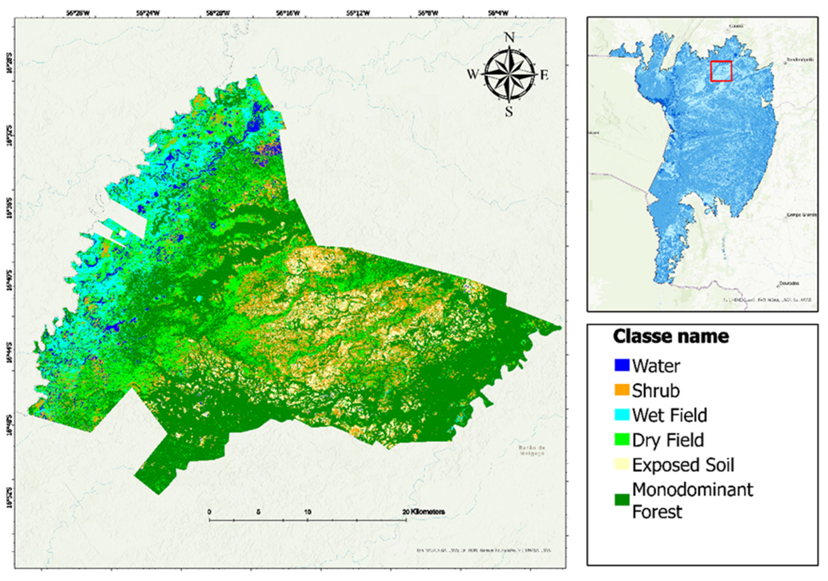
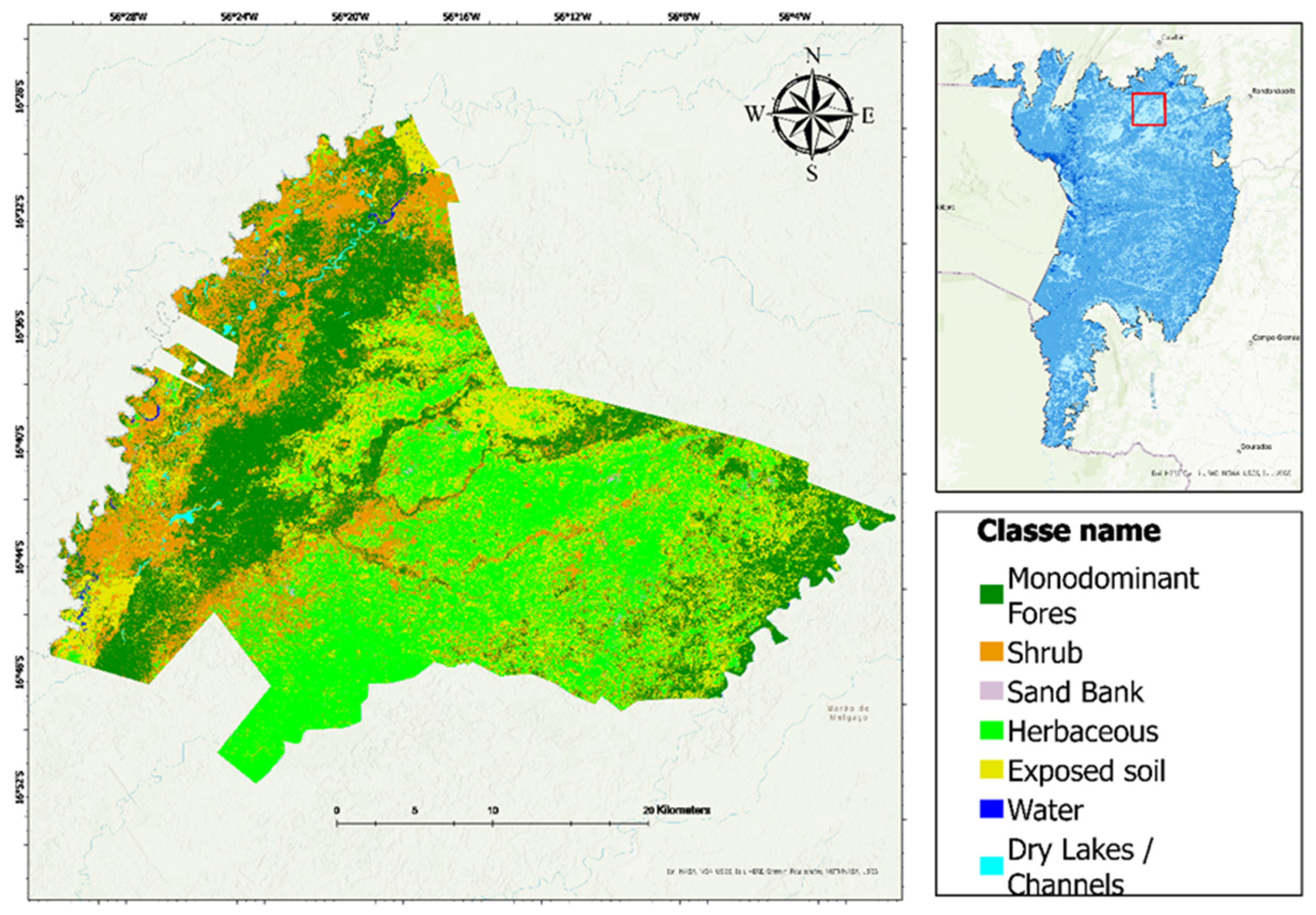
4.3. Supervised Classification Land Cover
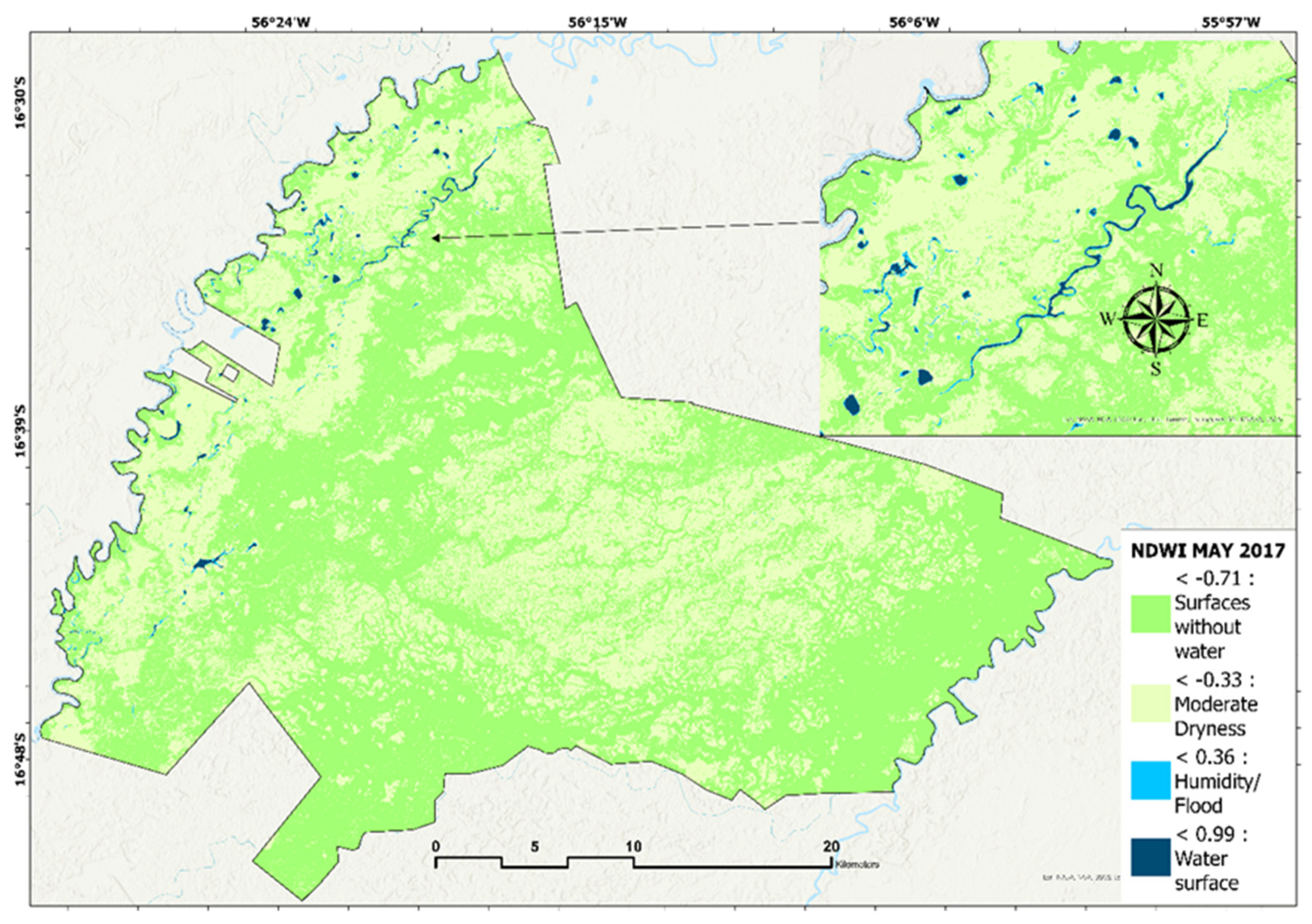
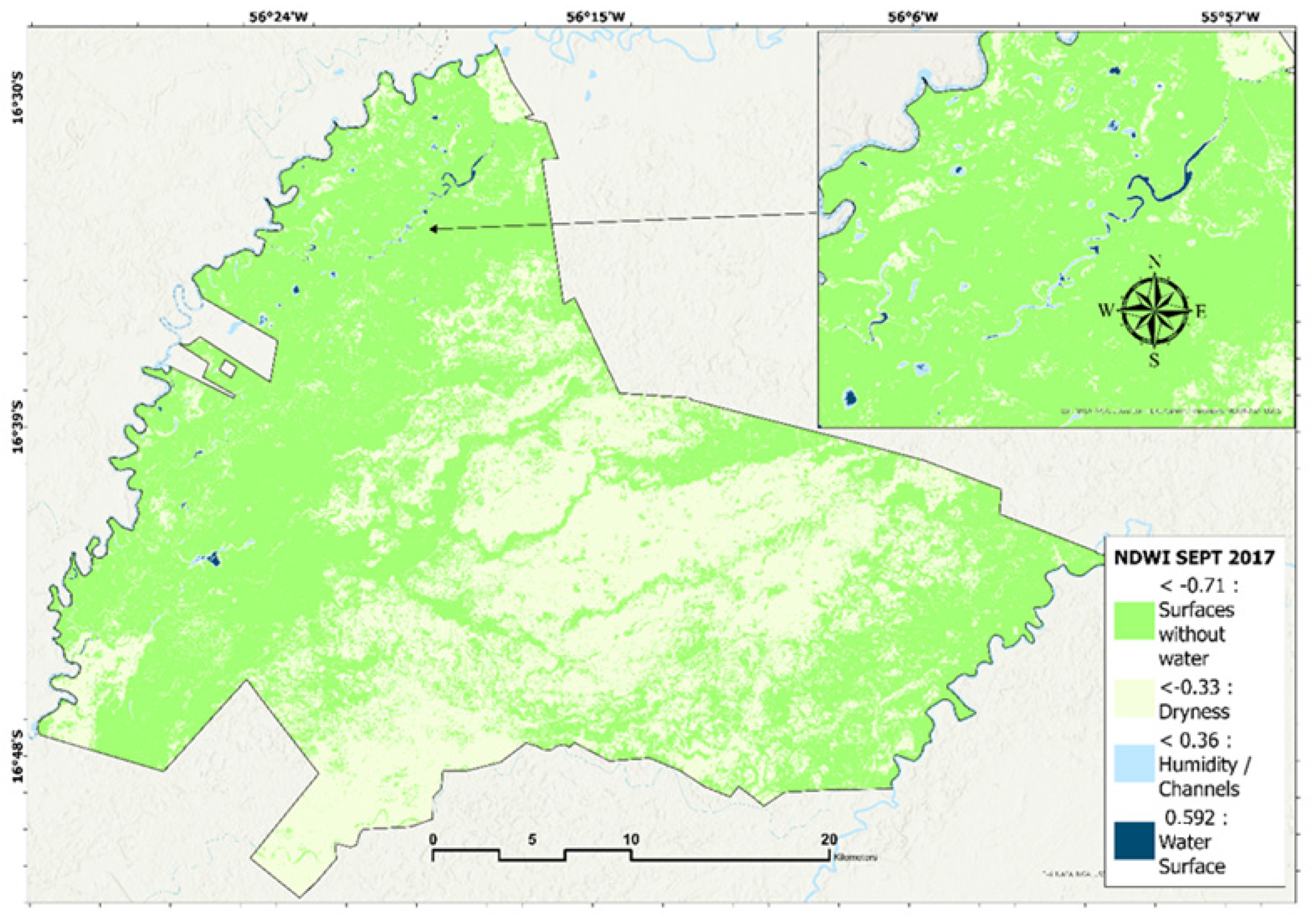
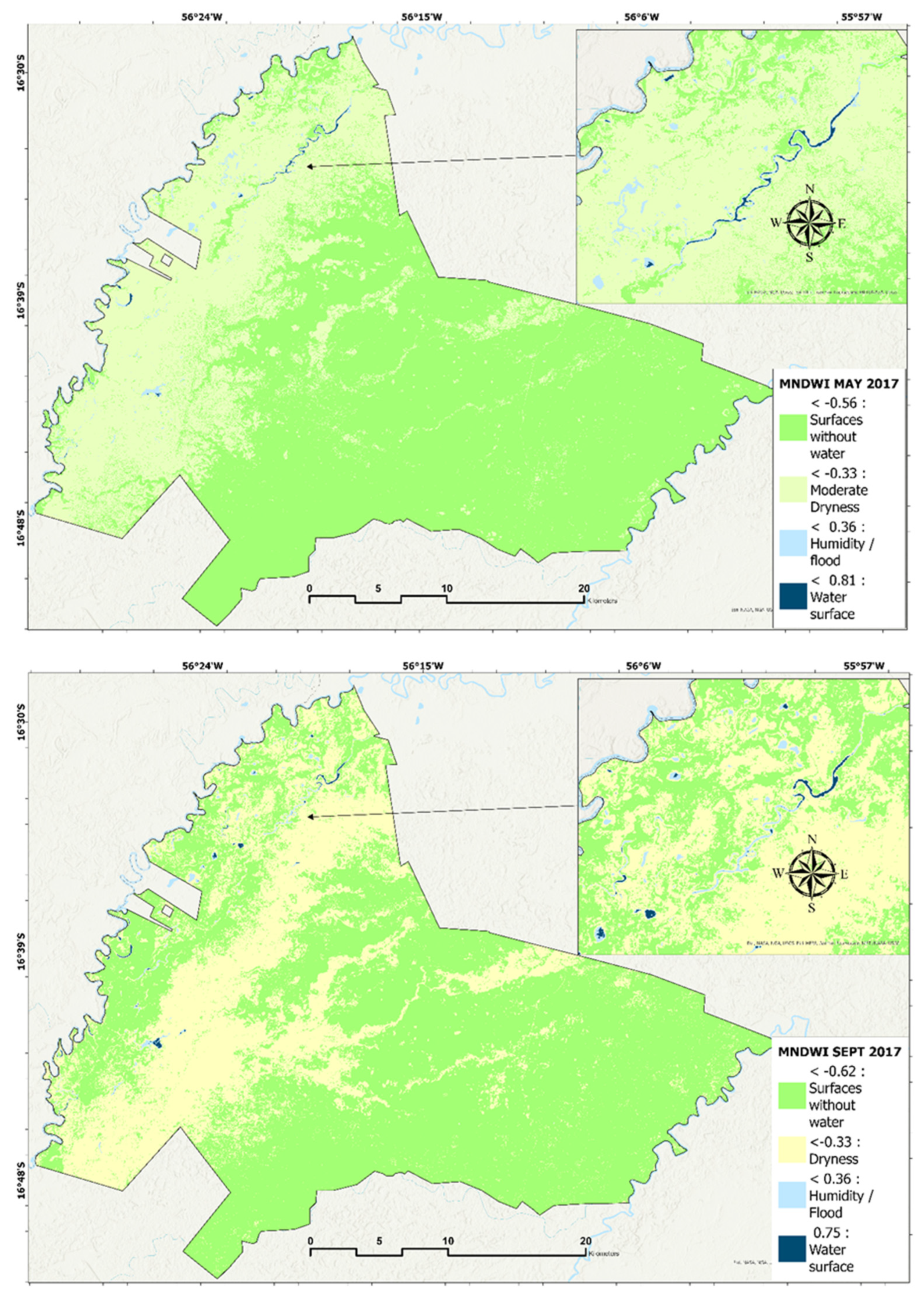
To identify the open water bodies in the study area, two land cover maps were produced based on supervised classification of the Sentinel-2 imagery using the SVM algorithm, selecting image dates with <10% cloud cover for the year 2017. Six environments were distinguished: water, shrub, dry field, exposed soil, flooded field, and dry forest/monodominant forest. The shrub and flooded field classes had the largest coverage in the Cuiabá River active floodplain.
The classification maps from SVM are displayed in Figure 5 and Figure 6. Both maps are based on imagery from May and September 2017 and were geographically coregistered with ground points, and specific land cover categories were further checked against independent observations. Overall, both maps show an accurate land cover classification, but there are significant differences between some classes. The shrub class showed differences between the two maps during the analyzed periods (wet season and dry season, specifically May and September 2017), with a greater dominance by shrubs in the dry season (the shrub canopy becomes partially submerged at high water).
This supervised land cover classification was designed to extract and highlight water bodies on the floodplain. As expected, the land cover map for May 2017 (high water) shows a larger area of open water than in September 2017 (dry season) (Figure 5 and Figure 6).

4.4. Water Indices

The distinct spectral reflectance of open water compared to dry land or vegetation allowed us to identify open water bodies using the NDWI (Figure 7).
During the study period, the month with the highest discharge was April 2017. However, due to the lack of cloud-free Sentinel-2 optical images then, the available imagery closest to the highest flood was from May 2017. The lowest discharge in 2017 was in September when cloud-free optical images were available. The NDWI for the May 2017 high-water period ranged from −0.71 to 0.99, while in the low-water September 2017 period it ranged from −0.71 to 0.59 (Figure 7). The most positive NDWI values correspond to open water, and values for the largest open water bodies were >0.5. Vegetation has much lower values, resulting in an easier distinction between vegetation and open water, although the Pantanal open water is often intermixed with emergent and floating vegetation, creating a continuum from open water to closed vegetation canopies above the water surface. Nevertheless, in the high-water period of May 2017, many water bodies, such as abandoned channels and meanders as well as small lakes, are visible on the floodplain. In the low-water period of September 2017, water bodies are still present, though their coverage is significantly lower.
In addition to the NDWI, open water bodies were also mapped by MNDWI (modified normalized difference water index). Figure 8 shows that the MNDWI values ranged between −0.80 and 0.75 in May 2017, the month with maximum river discharge that was possible to map with the Sentinel-2 images. In the month with the minimum river discharge (September 2017), the MNDWI ranged between −0.68 and 0.74.
Table 1 compares the frequency distributions in various classes of the water indices and land cover mapping in the study area. Based on the NDWI, we estimate that surface water covered 317.95 ha in May 2017 and 128.30 ha in September 2017, with the open water located principally in the active floodplain of the Cuiabá River (Table 1). The MNDWI estimated similar but lower total areas of 107.94 and 135.33 ha for those two months.

5. Discussion

The discharge data from the Porto Cercado station along the lower course of the Cuiabá River indicate that the discharge rises markedly during the rainy season between February and May, then falls abruptly and predictably to seasonal lows during the dry season between July and October (Figure 3). This dynamic is typical of the wet–dry climate at this latitude and is similar to most Pantanal rivers [13,40,41] Inundation of the Cuiabá River floodplain in the study area typically begins in December or January with peak flood in February and March, and hence, the flood duration is, on average, four months. In the most extensive flood during this study, as inferred from river discharge, the floodplain was not entirely inundated. At a particular location on the floodplain, the duration of flooding depends on the topographic level and the proximity to the main rivers or paleo-channels [11]. An average maximum annual flood duration of 172 days (5.6 months) was estimated by [11] for the Cuiabá sub-regions within which the present study area lies but those subregions also include land on the other sides of the Cuiabá river
The Cuiabá River hydrograph shows that the maximum discharge of ~600 m3/s occurred in April 2017 (Figure 3). Inundation of the active floodplain, while directly related to river discharge and water level, depends on the connectivity between the floodplain and the river [40]. In the study area, the active floodplain subject to inundation by the Cuiabá River is characterized as a lacustrine fluvial area consisting of recent alluvium formations, fluvial islands, marginal levees, and bars. Inundation of the active floodplain occurs every year, albeit to a variable degree.
Although extreme events play an essential role in restoring ecological succession and shaping floodplain geomorphology, more modest but frequent flood events (e.g., return periods of one to a few years) can determine the ecological structure and function and maintain greater overall biodiversity of the floodplain ecosystem [11].
The hydrological dynamics of the Cuiabá River floodplain system were studied in detail by [40,41]. They showed that during the wet season, water invaded the south side of the river through distributary channels. A levee about 70 m wide, parallel to the river, remained dry during the flood. At the beginning of the flood season, from December to January, the water level started to rise in the floodplain, originating from both direct rainfall and the rise of the Cuiabá River. The levees along the Cuiabá River channel constitute the highest local elevation and as such, are the last land to be flooded and the first to emerge. The water did not overflow the river’s levees but entered the floodplain through several small channels that cut through the levees [40]. There was only a weak relationship between floodplain land elevation above sea level and flood magnitude in the Cuiabá River floodplain, as shown by [11], and inundation of the floodplain was generally not in water level equilibrium with the nearest river channel.
The present study mapped the open water bodies in the Cuiabá River floodplain, based on the digital elevation model (DEM), land cover (LC) supervised classification, and two different water indices (NDWI, MNDWI). The DEM delineated the low-lying active floodplain and thus can indicate the potential location of the open water bodies on the floodplain as well as distinguish the active floodplain from the paleo-floodplain. The estimates of open water areas based on the LC classification and the two water indices were comparable except for open water in September 2017 when the LC classification yielded a much lower total area (Table 1). This may be explained by a more dominant effect of plant canopies in the LC classification, while the water indices may be more sensitive to water beneath openings in the canopy. The water indices may also be more sensitive to very wet soil with no standing water compared to the LC classification.
Hence, the water indices values were interpreted as follows: ≤0.99: water surface; ≤0.36: flooded/humidity ≤−0.3: moderate dryness, ≤−1: dry/surfaces without water. Note that the spectral bands of green and near-infrared were used in the above equations, unlike the NDWI proposed by [42]. The use of green and near-infrared bands has been shown to be better for the separation of flooded areas [43].

6. Conclusions

We conclude that open water areas can be mapped based on optical satellite imagery and normalized difference water indices despite the likely presence of floating and emergent aquatic vegetation and variable turbidity in these shallow waters. The original NDWI and the MNDWI gave comparable results. Comparison with LC classification showed broad agreement except for the September 2017 dry season when the LC indicated much lower coverage of open water. Which of these indicators of open water is more accurate cannot be determined without detailed field observations designed to understand the causes of these differences. Given the variability in vegetation growth forms and structure as well as turbidity in tropical floodplains, such as the Pantanal, such field calibration and validation should be site-specific and consider seasonality in both water levels and plant canopy development.

Author Contributions

Conceptualization, E.J.M. and C.N.D.C.; methodology, E.J.M., C.N.D.C., and G.M.N.; software, E.J.M. and G.M.N.; Validation, C.N.D.C., G.M.N., G.P. and S.K.H.; formal analysis, E.J.M., C.N.D.C. and G.M.N.; investigation, E.J.M. and C.N.D.C.; data curation, E.J.M. and G.M.N.; writing—original draft preparation, E.J.M. and C.N.D.C.; methodology, E.J.M.; writing—review and editing, G.P. and S.K.H.; visualization, G.P. and S.K.H.; supervision, C.N.D.C., G.M.N., G.P. and S.K.H. All authors have read and agreed to the published version of the manuscript.

Funding

This research was funded by the Coordenação de Aperfeiçoamento de Pessoal de Nível Superior “Capes” through a partnership with GCUB-OAS-PAEC for researcher mobility in ecology and biodiversity conservation at the Federal University of Mato-Grosso. grant number [8887.495657/2020-00].

Conflicts of Interest

The authors declare that they have no known competing financial interest or personal relationship that could have appeared to influence the work reported in this paper.

References

  1. Dinnin, M.; Van de Noort, R. Wetland Habitats, their Resource Potential and Exploitation: A Case Study from the Humber Wetlands. 1999, pp. 69–78. Available online: http://hdl.handle.net/10036/29874 (accessed on 21 January 2023).
  2. Acreman, M.; Holden, J. How wetlands affect floods. Wetlands 2013, 33, 773–786. [Google Scholar] [CrossRef] [Green Version]
  3. Costanza, R.; de Groot, R.; Sutton, P.; van der Ploeg, S.; Anderson, S.J.; Kubiszewski, I.; Farber, S.; Turner, R.K. Changes in the global value of ecosystem services. Glob. Environ. Chang. 2014, 26, 152–158. [Google Scholar] [CrossRef]
  4. de Groot, D.; Brander, L.; Max Finlayson, C. Wetland ecosystem services. Wetl. B. I Struct. Funct. Manag. Methods 2018, 13, 323–333. [Google Scholar] [CrossRef] [Green Version]
  5. Stefanidis, S.; Alexandridis, V.; Theodoridou, T. Flood Exposure of Residential Areas and Infrastructure in Greece. Hydrology 2022, 9, 145. [Google Scholar] [CrossRef]
  6. Pricope, N.G.; Shivers, G. Wetland Vulnerability Metrics as a Rapid Indicator in Identifying Nature-Based Solutions to Mitigate Coastal Flooding. Hydrology 2022, 9, 218. [Google Scholar] [CrossRef]
  7. Junk, W.J.; Nunes da Cunha, C.; da Silva, C.J.; Wantzen, K.M. The Pantanal: Ecology, Biodiversity and Sustainable Management of a Large Neotropical Seasonal Wetland; Junk, W.J., Nunes da Cunha, C., da Silva, C.J., Wantzen, K.M., Eds.; Pensoft: Sofia, Bulgaria; Moscow, Russia, 2011; ISBN 978-9546424921. Available online: https://hdl.handle.net/11858/00-001M-0000-000F-D3D6-4 (accessed on 27 March 2023).
  8. de Magalhães Neto, N.; Evangelista, H. Human Activity Behind the Unprecedented 2020 Wildfire in Brazilian Wetlands (Pantanal). Front. Environ. Sci. 2022, 10, 848. [Google Scholar] [CrossRef]
  9. Junk, W.J.; Bayley, P.B.; Sparks, R.E. The flood pulse concept in river-Floodplain systems. Can. Spec. Publ. Fish. Aquat. Sci. 1989, 106, 110–127. [Google Scholar]
  10. Hamilton, S.K.; de Souza, O.C.; Coutinho, M.E. Dynamics of floodplain inundation in the alluvial fan of the Taquari River (Pantanal, Brazil). SIL Proc. 1922–2010 1998, 26, 916–922. [Google Scholar] [CrossRef]
  11. Fantin-Cruz, I.; Pedrollo, O.; Castro, N.M.R.; Girard, P.; Zeilhofer, P.; Hamilton, S.K. Historical reconstruction of floodplain inundation in the Pantanal (Brazil) using neural networks. J. Hydrol. 2011, 399, 376–384. [Google Scholar] [CrossRef]
  12. Girard, P. Hydrology of surface and groundwaters in the Pantanal floodplains. In The Pantanal: Ecology, Biodiversity and Sustainable Management of a Large Neotropical Seasonal Wetland; 2011; pp. 103–126. Available online: https://www.amazon.com.br/Pantanal-Biodiversity-Sustainable-Management-Neotropical/dp/9546424927 (accessed on 27 March 2023).
  13. Pupim, F.D.N. Geomorfologia e Paleo-Hidrologia dos Megaleques dos Rios Cuiabá e São Lourenço, Quaternário da Bacia do Pantanal; Universidade Estadual Paulista: Rio Claro, Brazil, 2014. [Google Scholar]
  14. Fassoni-Andrade, A.C.; Fleischmann, A.S.; Papa, F.; de Paiva, R.C.D.; Wongchuig, S.; Melack, J.M.; Moreira, A.A.; Paris, A.; Ruhoff, A.; Barbosa, C.; et al. Amazon Hydrology From Space: Scientific Advances and Future Challenges. Rev. Geophys. 2021, 59, 97. [Google Scholar] [CrossRef]
  15. Guo, M.; Li, J.; Sheng, C.; Xu, J.; Wu, L. A review of wetland remote sensing. Sensors 2017, 17, 777. [Google Scholar] [CrossRef] [PubMed] [Green Version]
  16. Melack, J.M.; Hess, L.L. Remote Sensing of the Distribution and Extent of Wetlands in the Amazon Basin. In Amazonian Floodplain Forests: Ecophysiology, Biodiversity and Sustainable Managemen; Springer: Dordrecht, The Netherlands, 2010; Volume 210, pp. 43–59. ISBN 9789048187256. [Google Scholar]
  17. Dong, J.; Metternicht, G.; Hostert, P.; Fensholt, R.; Chowdhury, R.R. Remote sensing and geospatial technologies in support of a normative land system science: Status and prospects. Curr. Opin. Environ. Sustain. 2019, 38, 44–52. [Google Scholar] [CrossRef]
  18. Stefanidis, S.; Alexandridis, V.; Mallinis, G. A cloud-based mapping approach for assessing spatiotemporal changes in erosion dynamics due to biotic and abiotic disturbances in a Mediterranean Peri-Urban forest. CATENA 2022, 218, 106564. [Google Scholar] [CrossRef]
  19. Hamilton, S.K.; Sippel, S.J.; Melack, J.M. Inundation patterns in the Pantanal wetland of South America determined from passive microwave remote sensing. Arch. Hydrobiol. 1996, 137, 1–23. [Google Scholar] [CrossRef]
  20. Papa, F.; Prigent, C.; Aires, F.; Jimenez, C.; Rossow, W.B.; Matthews, E. Interannual variability of surface water extent at the global scale, 1993–2004. J. Geophys. Res. Atmos. 2010, 115, 1–17. [Google Scholar] [CrossRef]
  21. Dettmering, D.; Schwatke, C.; Boergens, E.; Seitz, F. Potential of ENVISAT radar altimetry for water level monitoring in the Pantanal wetland. Remote Sens. 2016, 8, 596. [Google Scholar] [CrossRef] [Green Version]
  22. Evans, T.L.; Costa, M.; Telmer, K.; Silva, T.S.F. Using ALOS/PALSAR and RADARSAT-2 to Map Land Cover and Seasonal Inundation in the Brazilian Pantanal. IEEE J. Sel. Top. Appl. Earth Obs. Remote Sens. 2010, 3, 560–575. [Google Scholar] [CrossRef]
  23. Padovani, C.R. Dinâmica Espaço-Temporal das Inundações do Pantanal; Universidade de São Paulo (USP): São Paulo, Brazil, 2010. [Google Scholar]
  24. da Paz, A.R.; Collischonn, W.; Tucci, C.E.M.; Padovani, C.R. Large-scale modelling of channel flow and floodplain inundation dynamics and its application to the Pantanal (Brazil). Hydrol. Process. 2011, 25, 1498–1516. [Google Scholar] [CrossRef]
  25. da Cunha, C.N.; Junk, W.J.; Fiuza, A.G.; Bononi, J.; de Arruda, E.C. Sítio Ransar | Sesc Pantanal; Cuibá, 2019. [Google Scholar]
  26. Lacerda Filho, J.V.D.; Abreu Filho, W.; Valente, C.R.; Oliveira, C.C.D.; Albuquerque, M.C.D. Geologia e Recursos Minerais do Estado de Mato Grosso; Programa Geologia do Brasil: Cuiabá, Brazil, 2004; p. 1976. [Google Scholar]
  27. Luis, M. Sedimentação na bacia do Pantanal Mato-Grossense, Centro-Oeste do Brasil. 2003. x, 106 f. Tese (livre-docência)—Universidade Estadual Paulista, Instituto de Geociências e Ciências Exatas. 2003. Available online: http://hdl.handle.net/11449/108382 (accessed on 27 March 2023).
  28. Nunes da Cunha, C.; Piedade, M.T.F.; Junk, W.J. Classificação e Delineamento das Áreas Úmidas Brasileiras e de seus Macrohabitats; EdUFMT: Cuiabá, Brazil, 2015; Volume 1, ISBN 9788578110796. [Google Scholar]
  29. ESA ESA’s Optical High-Resolution Mission for GMES Operational Services; European Space Agency: Paris, France, 2015; ISBN 9789292214197.
  30. Penha, T.V.; Pletsch, M.A.J.S.; Silva, C.H.L.; Körting, T.S.; Fonseca, L.M.G. Detecção e delimitação automática de corpos hídricos em imagens Sentinel-2: Uma proposta de integração do algoritmo Fmask aos índices espectrais NDWI e MNDWI. In Proceedings of the Anais do XVIII GEOINFO, El Salvador, December 2017; pp. 340–345. [Google Scholar]
  31. Vanhellemont, Q.; Ruddick, K. Acolite for Sentinel-2: Aquatic applications of MSI imagery. In Proceedings of the 2016 ESA Living Planet Symposium, Prague, Czech Republic, 9–13 May 2016; Volume SP-740, pp. 9–13. [Google Scholar]
  32. Eito-Brun, R.; Ledesma Rodríguez, M. 50 years of space research in Europe: A bibliometric profile of the European Space Agency (ESA). Scientometrics 2016, 109, 551–576. [Google Scholar] [CrossRef]
  33. McFeeters, S.K. Using the normalized difference water index (ndwi) within a geographic information system to detect swimming pools for mosquito abatement: A practical approach. Remote Sens. 2013, 5, 3544–3561. [Google Scholar] [CrossRef] [Green Version]
  34. Xu, H. Modification of normalised difference water index (NDWI) to enhance open water features in remotely sensed imagery. Int. J. Remote Sens. 2006, 27, 3025–3033. [Google Scholar] [CrossRef]
  35. McFeeters, S.K. The use of the Normalized Difference Water Index (NDWI) in the delineation of open water features. Int. J. Remote Sens. 1996, 17, 1425–1432. [Google Scholar] [CrossRef]
  36. Ponzoni, F.J.; Galvão, L.S.; Epiphanio, J.C.N. Spatial resolution influence on the identification of land cover classes in the Amazon environment. An. Acad. Bras. Cienc. 2002, 74, 717–725. [Google Scholar] [CrossRef] [Green Version]
  37. Jensen, J.R. Introdcutory Digital Image Processing: A Remote Sensing Perspective, 3rd ed.; Daniel, E., Kaveney, J.C., Eds.; Inc., Prentice-Hall: Upper Saddle River, NJ, USA, 2005; ISBN 0132058405. [Google Scholar]
  38. Landis, R.; Koch, G. An Application of Hierarchical Kappa-type Statistics in the Assessment of Majority Agreement among Multiple Observers. Biometrics 1977, 33, 363–374. Available online: https://www.jstor.org/stab (accessed on 23 April 2023). [CrossRef]
  39. Mohd Razali, N.; Bee Wah, Y. Power comparisons of Shapiro-Wilk, Kolmogorov-Smirnov, Lilliefors and Anderson-Darling tests. J. Stat. Model. Anal. 2011, 2, 21–33. [Google Scholar]
  40. Girard, P.; Da Silva, C.J.; Abdo, M. River-Groundwater interactions in the Brazilian Pantanal. The case of the Cuiabá River. J. Hydrol. 2003, 283, 57–66. [Google Scholar] [CrossRef]
  41. Girard, P.; Fantin-Cruz, I.; de Oliveira, S.M.L.; Hamilton, S.K. Small-scale spatial variation of inundation dynamics in a floodplain of the Pantanal (Brazil). Hydrobiologia 2010, 638, 223–233. [Google Scholar] [CrossRef]
  42. Gao, B.-C. NDWI—A normalized difference water index for remote sensing of vegetation liquid water from space. Remote Sens. Environ. 1996, 58, 257–266. [Google Scholar] [CrossRef]
  43. Brenner, V.C.; Guasselli, L.A. Índice de Diferença Normalizada da Água (NDWI) para Identificação de Meandros Ativos no Leito do Canal do Rio Gravataí/RS-Brasil; Anais XVII Simpósio Brasileiro de Sensoriamento Remoto-SBSR: João Pessoa, Brasil, 2015; pp. 6381–6388. [Google Scholar]
Figure 1. Map of the SESC Pantanal study area (left) and its location within the Pantanal and South America.
Water 15 02180 g001
Figure 2. Methodological flowchart.
Water 15 02180 g002
Figure 3. Mean monthly discharge for the São Lourenço and Cuiabá rivers during 2015–2020. Data obtained from the fluviometric stations at Porto Cercado on the Cuiabá River (river station code: 66340000) and at the Acima do Córrego Grande on the São Lourenço River (river station code: 66460000).
Water 15 02180 g003
Figure 4. Hypsometric map of the study site. Image with UTM coordinate system, Datum SIRGAS 2000, zone 21 S.
Water 15 02180 g004
Figure 5. Land cover classification based on imagery from the high-water period (May 2017) in the study area. Image made with UTM coordinate system, Datum SIRGAS 2000 zone 21 S.
Water 15 02180 g005
Figure 6. Land cover classification based on imagery from the low water period (September 2017) in the study area. Image made with UTM coordinate system, Datum SIRGAS 2000 zone 21 S.
Water 15 02180 g006
Figure 7. Normalized difference water index (NDWI) in the study area (main map) and along the Cuiabá River (inset) in months representing high water in the river (top; May 2017) and low water (bottom; September 2017). Open water areas are highlighted in blue. Image made with UTM coordinates system, Datum SIRGAS 2000 zone 21 S.
Water 15 02180 g007aWater 15 02180 g007b
Figure 8. Modified normalized difference water index (MNDWI) in the study area (main map) and along the Cuiabá River (inset) in months representing high water in the river (top; May 2017) and low water (bottom; September 2017). Open water areas are highlighted in blue. Image made with UTM coordinate system, Datum SIRGAS 2000 zone 21 S.
Water 15 02180 g008
Table 1. Imagery. The total area of the study site is 108,095.3 ha within which the active floodplain of the Cuiabá River covers 26,033 ha.
Method of EstimationPeriodClassesArea (ha)Area (%)Kruskal-Wallis Test
Surfaces without water63,962.7459.17
Moderate dryness43,525.2540.27
May 2017Humidity/flood289.390.27
Water surface317.950.29
NDWI Surfaces without water63,587.8558.83
Moderate dryness44,075.4740.77
September 2017Humidity/flood303.710.28
water surface128.300.12
Surfaces without water71,377.9766.03p-value = 0.4514
May 2017Moderate dryness36,038.3633.34
Humidity/flood571.060.53
water surface107.940.10
MNDWI Surfaces without water72,471.2667.04
Moderate dryness35,005.5932.38
September 2017Humidity/flood483.150.45
water surface135.330.13
Monodominant forest52,742.9848.79
Shrub13,222.4912.23
Sazonal herbaceous9528.178.81
Land CoverMay 2017Exposed soil6794.516.29
Water3325.863.08
Humidity/flood22,481.4520.80
Monodominant forest29,259.6527.07
Shrub21,794.2520.16
Land CoverSeptember 2017Sazonal dry field32,554.4630.12
Exposed soil23,360.4521.61
Water198.030.18
Dry field526.840.49
Disclaimer/Publisher’s Note: The statements, opinions and data contained in all publications are solely those of the individual author(s) and contributor(s) and not of MDPI and/or the editor(s). MDPI and/or the editor(s) disclaim responsibility for any injury to people or property resulting from any ideas, methods, instructions or products referred to in the content.

