Turbulence Kinetic Energy and High-Order Moments of Velocity Fluctuations of Flows in the Presence of Submerged Vegetation in Pools

Abstract

The flow in arid and semi-arid regions changes significantly during seasons, letting many vegetation patches develop in different parts of rivers. In the presence of aquatic plants in streams, different flow structures have resulted. When the water level increases in these rivers, the presence of vegetation patches influences the turbulent flow structures, which may considerably change the estimation of key hydraulic parameters. The results of earlier investigations indicated that a wide range of submerged and non-submerged vegetation influences the hydrodynamic features of flows in rivers and streams. In the present investigation, two pools with various slopes of entry and exit sections were used to conduct eight independent experiment runs. In addition, a vegetation patch over the entire pool section has been set up to investigate the effects of the vegetation patch on flow structures in pools. The effect of two slopes of 5 and 10 degrees for both entrance and exit of the pools on flow structure has been investigated. Considering two aspect ratios of 2.0 and 2.7, the distributions of flow velocity, Reynolds normal and shear stresses, turbulence intensities, turbulent kinetic energy (TKE), quadrant analysis, and spectral analysis have been studied at the trailing edge of the vegetation patch along an artificial pool. Results show that, for large entrance and exit slopes (10 degrees), the TKE distribution profiles have no specific form. However, the TKE values have a convex-shaped distribution pattern with the maximum TKE value near the bed when the slopes of the entrance and exit sections of the pool are small (5 degrees). Results showed that both ejections and sweeps govern the turbulence structures and coherent motions at the trailing edge of the vegetation patch along the pool. The geometry, entrance, and exit slopes of the pool have no effect on the validation of power spectral function compared to the presence of a vegetation patch in a flatbed.

1. Introduction

In wetland environments, the channel beds of streams or rivers are commonly covered by either partially or fully submerged diverse aquatic plants, such as grasses, shrubs, and bushes. Both vegetated and non-vegetated zones in these streams significantly influence the hydrodynamic features of the flow, such as velocity distributions, turbulence intensity, and coherent structures, as well as mass and momentum exchange. To date, a variety of research works have been published with respect to the flow structures [1,2,3,4].

Due to the interaction of the vegetated zone and main channel, the vertical distribution profile of the streamwise velocity follows an S-shape, which is caused by the secondary currents in a narrow channel created by riparian vegetation. In fact, an S-shaped velocity profile indicates that there are two vertical mixing layers with coherent structures induced by the development of vertical shear stress, resulting in variations of flow velocities in both longitudinal and vertical directions. The characteristics of the horizontal coherent structures near the vegetation boundary and main flow interface are also influenced by secondary transversal velocity, and different inclination directions of these coherent structures are observed at different depths corresponding to the local transversal velocity [5]. Furthermore, zones of accelerating and decelerating flows in a river are generated due to the changes in its depth and width. Given the significant impact of these factors on turbulence generation and sediment transport, a variety of river topographies, particularly pools and riffles, would be developed [6,7,8]. To assess the effects caused by a vegetation canopy and a pool bed, turbulence structures and coherent motions of the bursting process have been investigated in the present study. Turbulent flow structures generated by the channel bed and vegetation cover are significantly more complex in conditions with bank vegetation than that with submerged vegetation [9,10].

To investigate turbulence structures above the vegetation canopy, the turbulent kinetic energy (TKE) should be examined, and then the shear and wake generation can be estimated [11]. It should be noted that the wake production is the horizontal average of the product of the local variations of Reynolds stresses and velocity gradients. As reported by the previous researchers, the shear velocity in the presence of vegetation yields more turbulent energy than that caused by the wake of vegetation, except for those zones around the edge of the vegetation patches [12,13]. Furthermore, the presence of vortexes leads to an increase in the TKE [3,14,15,16]. In 2D flows in channels with emergent vegetation elements, instabilities caused by horizontal vortexes at the downstream edge of a vegetation patch play a dominant role in flow structures [17,18]. In the presence of a vegetation canopy layer in a flow, an analogy between the canopy layer and the flow’s mixing layer has been reported [19,20].

In the near-bed region, by means of the quadrant analysis, the occurrence probabilities are dominated by the presence of sweep motions and depend on the thickness density of the vegetation patch, which causes a larger wake zone in the emergent region over the canopy. The majority of reported studies focused on evaluating the structures of coherent flows above a vegetation patch [4,5]. In the present study, coherent flow structures have been investigated upstream of the vegetation patch, across the entire vegetation patch in a pool (compared to those in a pool without vegetation), and at the vegetation canopy boundary. It has been found that the motion of ejections appears behind the vegetation patch. The dominant bursting process in flows over vegetation canopy belongs to the periodic occurrence of sweep and ejection events. A variety of research works has been conducted to study the interactions between strong vortices above vegetation canopies and quadrant occurrences [11]. This study’s results of high-order moments of velocity fluctuations u’ and w’, also known as skewness fluctuations ${\mathrm{sk}}_{\mathrm{u}}$ and ${\mathrm{sk}}_{\mathrm{w}}$, can be used to derive factors that provide useful information about asymmetry in streams [18]. In other words, a non-zero skewness of velocity fluctuations in the streamwise and vertical directions indicates an asymmetric probability density function (PDF) of the considered variable, which is associated with quadrant bursting events [21].

In practice, engineers are keen on the estimation of low resistance along a pool in the presence of vegetation in a channel bed since the resistance changes along different sections of a pool, including both entrance and exit slopes as well as different locations inside the vegetation patch. To the authors’ knowledge, no research work has been reported on the investigation of the details of flow structures (including 3D velocity components distributions, 3D turbulence intensities, and turbulence kinetic energy distributions) at the trailing edge of vegetation patch (where the flow reach to gravel along a stream) in the presence of bed forms. Moreover, the application of the power spectral density of velocity components over 3D bed forms in the presence of vegetation patches in the channel bed and the validation of Kolomogrove −5/3 law has been investigated in this study.

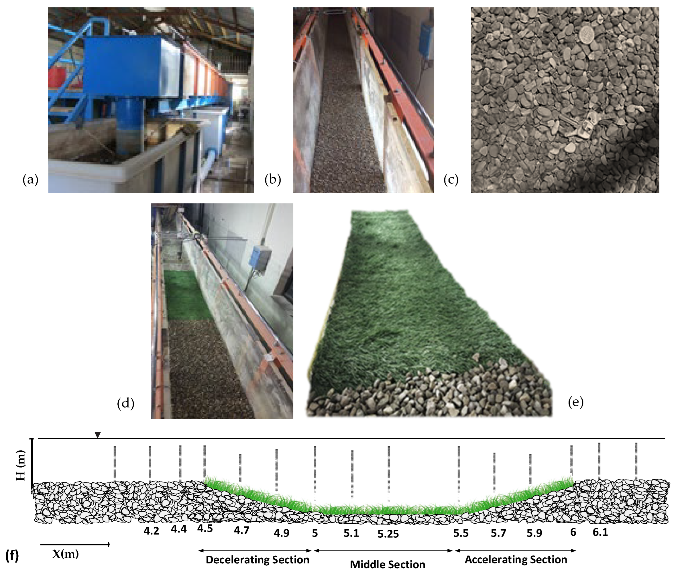
2. Materials and Methods

In the present study, the desired two pool bed forms were built in a laboratory flume, which is 8-m long, 0.4-m wide, and 0.6-m deep. One was built with a constant slope of 5 degrees for both the entrance and exit sections, while the other was built with a constant slope of 10 degrees for both the entrance and exit sections. All experiment runs have been conducted with vegetation in the pools and without vegetation in the pools (Figure 1). For this experimental study, each desired pool bed form was set up in a section of the flume to ensure that the flow was under fully developed conditions. To avoid the effects of the downstream tailgate, the 1.5-m long pool was built at a distance of 4.5 m from the entrance of the flume. The tailgate located downstream end of the flume was used to control the flow depth and maintain the desired flow depth of 20 cm and 15 cm, respectively (

Table 1. Experimental Conditions.

Pool Setup	Runs.	Entrance Slope	Exit Slope	$\mathbf{H} \left(\mathbf{c}\mathbf{m}\right)$	Pool-Bed Material	U (m/s)	$\mathbf{Q}$ $(\mathbf{lit}/\mathbf{s})$	${\mathit{F}}_{\mathit{r}}$	$\mathit{R}\mathit{e} \mathbf{(}{\mathbf{10}}^{\mathbf{4}}\mathbf{)}$	w/h	$\mathbf{H}/{\mathit{d}}_{50}$
Setup 1	Run 1	5°	5°	20	Gravel Bed	0.125	10.5 ± 0.1	0.09	2.5	2	20
	Run 2	5°	5°	20	Gravel Bed	0.5	40.5 ± 0.1	0.13	10	2	20
	Run 3	5°	5°	20	Vegetated Canopy	0.125	10.5 ± 0.1	0.09	2.5	2	-
	Run 4	5°	5°	20	Vegetated Canopy	0.5	40.5 ± 0.1	0.13	10	2	-
Setup 2	Run 5	10°	10°	20	Gravel Bed	0.125	10.5 ± 0.1	0.09	2.5	2	20
	Run 6	10°	10°	20	Vegetated Canopy	0.125	10.5 ± 0.1	0.09	2.5	2	-
	Run 7	10°	10°	15	Vegetated Canopy	0.125	10.5 ± 0.1	0.09	2.5	2.67	-
	Run 8	10°	10°	20	Vegetated Canopy	0.125	10.5 ± 0.1	0.09	2.5	2	-

). A water gauge mounted on the channel walls is used to determine the water depth.

The median diameter of bed material $\left({\mathrm{d}}_{50}\right)$ in the pool bed for all experiments is ${\mathrm{d}}_{50}$ = 10.4 mm, which is determined by using one hundred random samples of the grains. The results of the grain size distribution show that the bed material is relatively non-uniform according to the geometric standard deviation ${\mathsf{\sigma }}_{\mathrm{g}}{=(\mathrm{d}}_{84}{/\mathrm{d}}_{16}{)}^{0.5}$, where ${\mathrm{d}}_{16}$ and ${\mathrm{d}}_{84}$ are the 16th and 84th percentile of the particle-size distribution, respectively. In this study, the geometric standard deviation is smaller than 1.4, indicating that the bed material is non-monotonous. Figure 2 shows the grain size distribution curve, and the particle characteristics for this experiment are determined through the following method (

Table 2. Characteristics of bed material.

Parameters	${\sigma }_g$	${\mathbf{G}}_{\mathbf{r}}$	${\mathbf{D}}_{\mathbf{g}}$	${\mathbf{C}}_{\mathbf{c}}$	${\mathbf{C}}_{\mathbf{u}}$	${\mathrm{d}}_{10}$	${\mathrm{d}}_{16}$	${\mathrm{d}}_{30}$	${\mathrm{d}}_{50}$	${\mathrm{d}}_{60}$	${\mathrm{d}}_{84}$
Sum.	1.17	1.17	4.6	0.95	1.22	8.8	9	9.5	10.4	10.8	12.3

). The granulation coefficient $\left({\mathbf{G}}_{\mathbf{r}}\right)$ is determined by $(-0.5)({\mathrm{d}}_{84}/{\mathrm{d}}_{50}+{\mathrm{d}}_{50}/{\mathrm{d}}_{16})$; the average particle size (${\mathbf{D}}_{\mathbf{g}}$) depicts as ${({\mathrm{d}}_{84}/{\mathrm{d}}_{16})}^{0.5}$; ${\mathbf{C}}_{\mathbf{c}}$ indicates the curvature coefficient calculated by ${\left({\mathrm{d}}_{30}\right)}^2/({\mathrm{d}}_{10} \times {\mathrm{d}}_{60})$, and ${\mathbf{C}}_{\mathbf{u}}$ represents the uniformity coefficient calculated by $({\mathrm{d}}_{60}/{\mathrm{d}}_{10})$.

The vegetation selected for this experimental study was a 2-cm tall artificial grass patch (measured under dry conditions) that covers the entire pool section of the flume. Table 2 summarizes data collected from all experimental runs. The experiments conducted in the pool with the 5-degree slope for both entrance and exit sections have been carried out for two different discharges of 10.5 and 40.5 lit/s. The experiments conducted in the pool with the 10-degree slope were carried out under two different aspect ratios (w/h; channel width to water depth) of w/h = 2 and 2.7. Along with the aforementioned information, Table 2 also presents the flow Froude number; $\mathrm{Fr}=[\mathrm{U}/{\left(\mathrm{gH}\right)}^{0.5}]$, and the flow Reynolds number; $\mathrm{Re}[=\mathrm{UH}/v_{\mathrm{m}}]$, where H is the water depth; U is mean velocity, and $v_{\mathrm{m}}$ is the flow kinematic viscosity. An electromagnetic flowmeter installed at the water pipe entering the flume was used to measure flow discharge.

A Nortek Vectrino Acoustic Doppler Velocimeter (ADV) was used to measure the instantaneous three-dimensional velocity components. For each experimental run, the ADV (Acoustic Doppler velocimeter) was used to measure the flow velocity at the distance of z = 2 mm from the bed to 50 mm below the water surface. Even though some data were filtered to remove outliers, most of the velocity data collected in this study was examined with high SNR (signal-to-noise ratio) and correlation. To investigate secondary currents, data for Run 8 were collected along the channel’s second axis, which was located 10 cm away from the flume side wall, whereas data collected for all other experimental runs were obtained along the flume’s center line (20 cm from the flume sidewalls).

3. Results

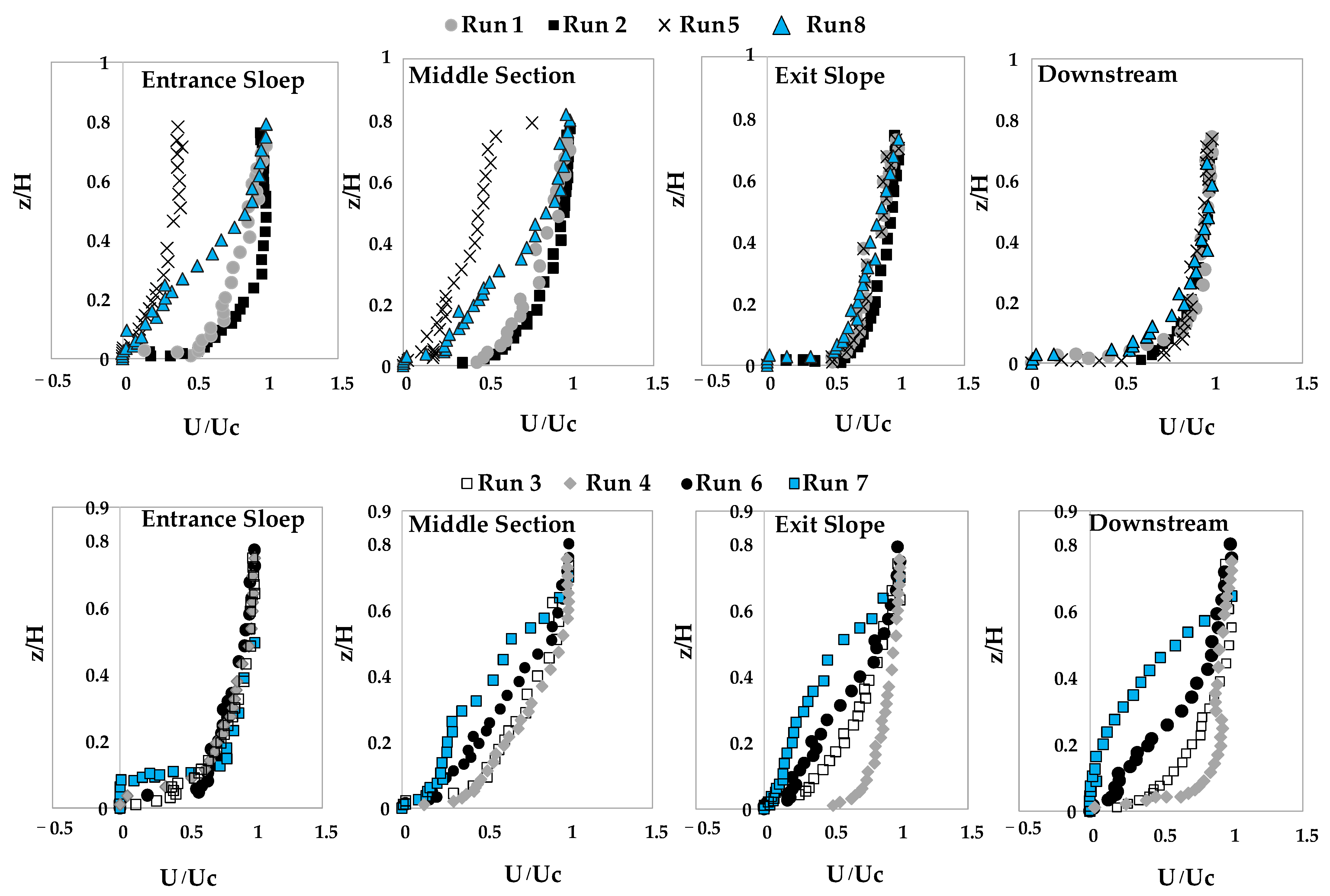
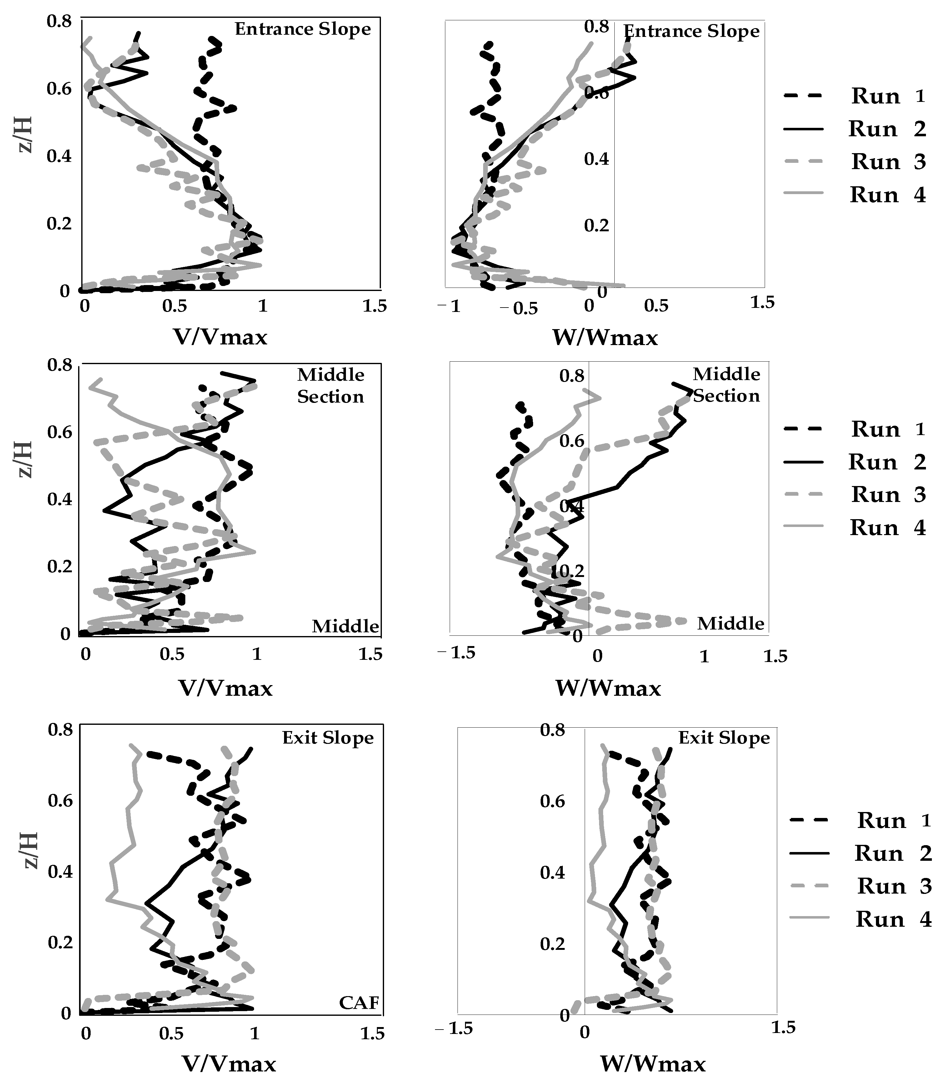
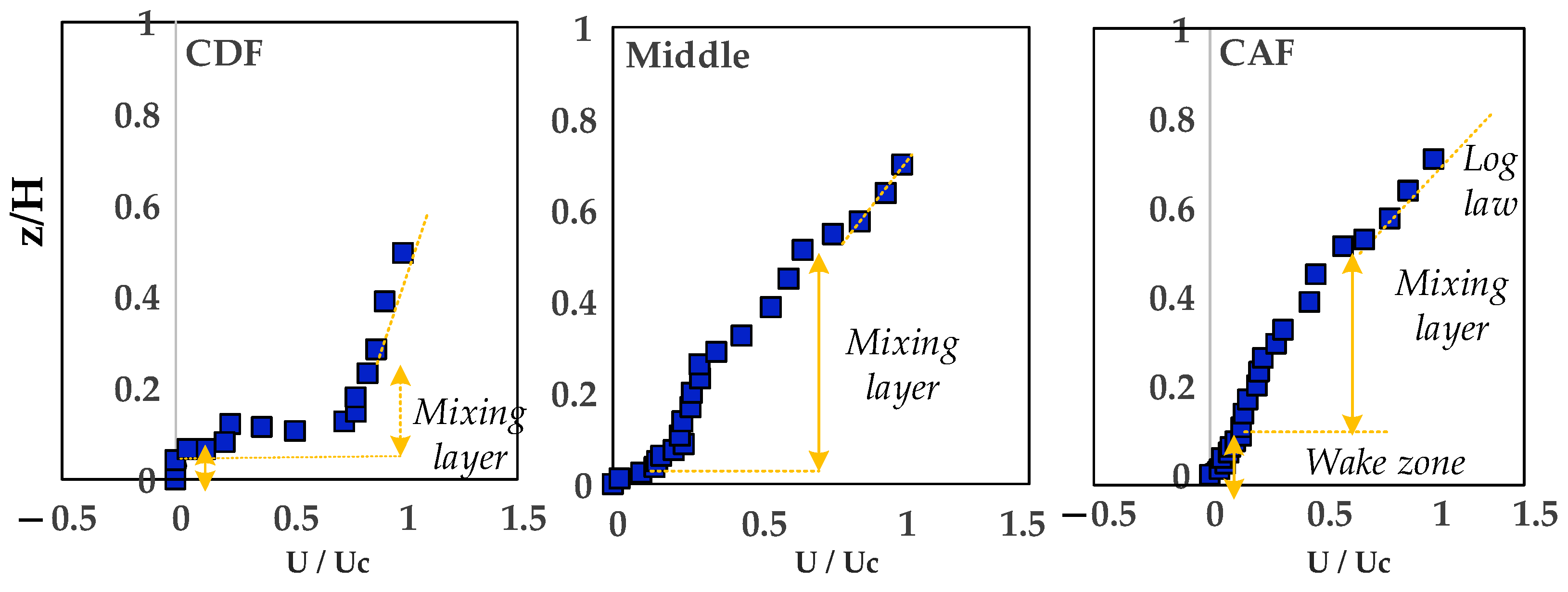
3.1. Velocity Distribution

As shown in Figure 3, the stream-wise velocity (x direction) profiles of 3D flows are displayed for all experimental runs. At each measurement point, the mean point velocity is divided by the maximum flow velocity (u_c) of the profile, and each depth from the bed (z) is divided by the flow depth (H); in this way, the dimensionless velocity (u/u_c) and flow depth (z/H) are obtained, respectively (Figure 3). As the water depth rises on the entrance slope, the flow velocity decreases, creating a decelerating flow section (CDF) over the pool’s entrance section. The accelerating flow (CAF) develops at the end of the middle pool section, where the water depth decreases along the exit slope of the bed. For the flow with a low aspect ratio (flume width/flow depth H/B < 5), the location of the maximum velocity may fluctuate due to the influence of secondary currents. However, with a greater aspect ratio (H/B > 5), this effect is hardly noticeable. If the aspect ratio is less than 5, the dip phenomenon occurs, and the flow will be 3D [22,23]. Neither negative velocities nor flow separation at the bed of both entrance and exit sections of pools could be recorded because of the limitations of the ADV. As can be seen in Figure 3, there are different velocity profiles for flow in the pools with the change in the bed slope. However, flow velocities in the pool with a slope of 10 degrees are slower than those with a slope of 5 degrees. In a decelerating flow, the near-bed velocities are lower than those at the water surface are, and this discrepancy increases in the streamwise direction.

The effect of decelerating flow is still present in the middle pool section, preventing the development of a uniform flow. In the accelerating flow, velocity increases near the bed and decreases near the water surface as the flow continues along the exit section of a pool.

Despite the aspect ratios being less than 5, no evidence for the velocity dip phenomenon is observed within the range of flow depth of z/h < 0.6. Nevertheless, the highest flow velocity has been observed below the water surface at a depth of z/H > 0.6 along the decelerating flow section when the entrance slope is 5 degrees (Figure 3). As the flow enters the pool region, the maximum flow velocity moves toward the water surface in the zone of flow depth of z/h > 0.8. This finding agrees well with the reported result that the dip phenomenon occurs at a distance up to 0.67 H (or dip parameter) from the bed for uniform flow with a hydraulic rough bed [21]. According to some earlier studies, the value of the dip parameter for non-uniform flows is 0.22 H [22]. In a gravel bed river with flexible submerged vegetation patches and 3D bed forms, this value is up to 0.8 H [24]. However, the findings of the theoretical investigations based on the Navier–Stokes equations demonstrate that the value of the dip parameter in an accelerating flow is higher than that in both uniform and decelerating flows [6].

According to this research, as depicted in Figure 3, the velocity fluctuation is primarily dependent on the drag force caused by the vegetation in the zone up to a depth of z/H = 0.1 in the pool, and the viscous shear stress has only a minor impact on the velocity profile, leading to minimal changes in the velocity profile. The velocity profile in the upper layer of the flow (z/H > 0.1) increases gradually with the flow depth (z/H). With increasing the aspect ratio, the presence of vegetation canopy inside the pool can result in an S-shaped distribution profile of velocity. This is true for both pool entry and exit sections with a slope of 10 degrees (decreasing the water depth from 20 cm to 15 cm). In fact, the velocity gradient in the upper layer of the flow approaches null; the velocity gradient reaches the maximum in the middle and close to the bed, and the velocity distribution follows the logarithmic function. This outcome supports the findings of prior research [22]. Moreover, contrary to what was found in earlier research, the dimensionless flow velocities in the outer zone of the decelerating flow section (z/h > 0.2) are not necessarily higher than those in the accelerating flow section, and some discrepancies have been observed in the aforementioned trends. [25,26,27]. To further assess the impacts of secondary currents on the characteristics of flow in a pool with the presence of vegetation, flow velocity components in the other two directions (span-wise v and vertical direction w) are shown for four experimental runs in Figure 4.

The presence of both positive and negative values of velocity profiles in both span-wise and vertical directions indicates the pattern of the secondary currents [5,23]. While the average vertical velocity is negative in the decelerating and middle sections of the pool, revealing the occurrence of a downward flow, the positive values of vertical velocities in the accelerating section indicate the inclination of flow toward the water surface. The opposing effect of accelerating and decelerating stream portions on secondary currents along the pool bed has been noted by a number of researchers, which led to the flow convergence along the entrance slope and flow divergence along the exit slope section of the flow [7], despite the fact that in a balanced flow, it is not always the case that the vertical velocity is downward in an accelerating flow and upward in a decelerating flow [26]. The convergence and divergence patterns of the flow in the deceleration and acceleration sections are in agreement with field investigations and experimental studies [28,29].

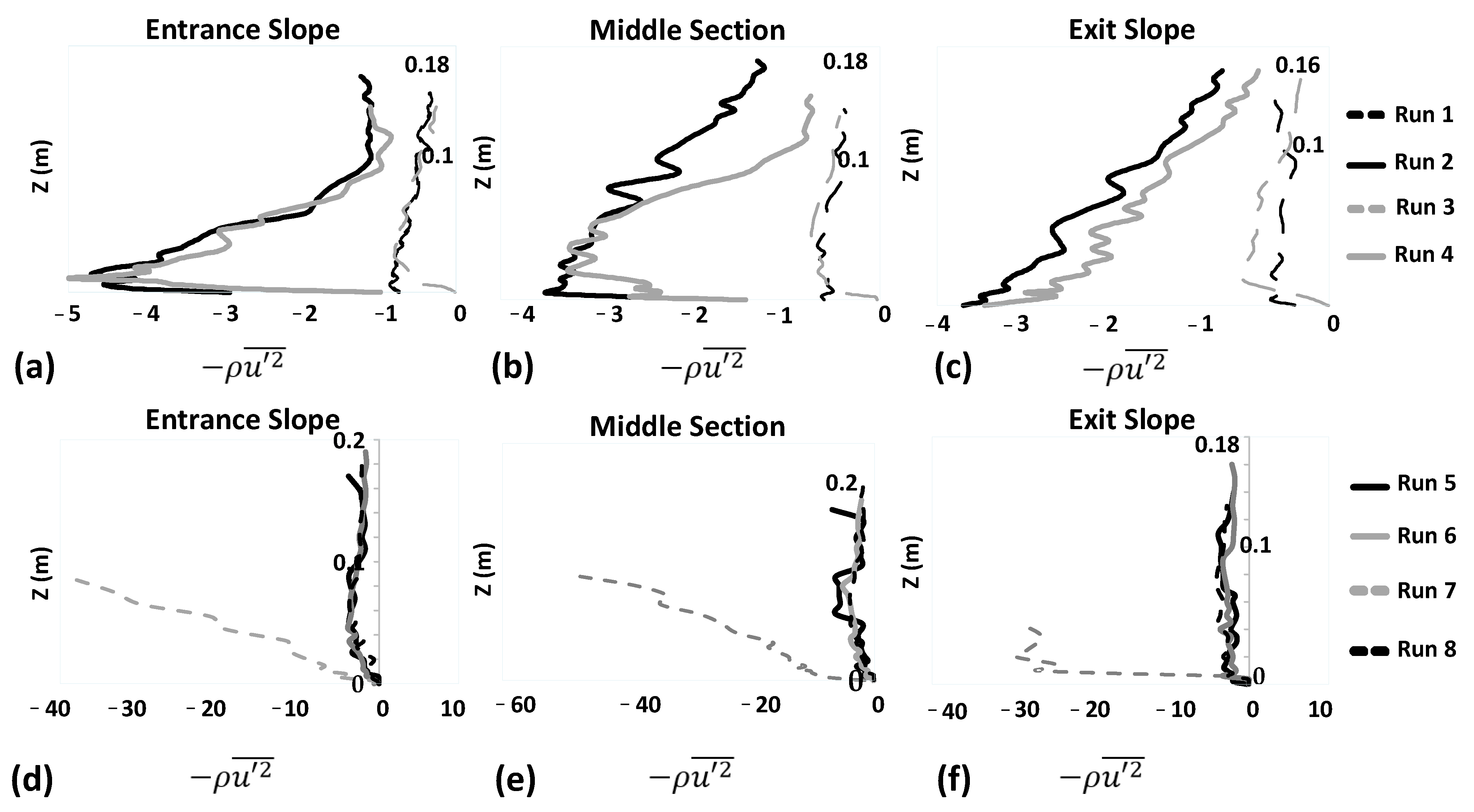
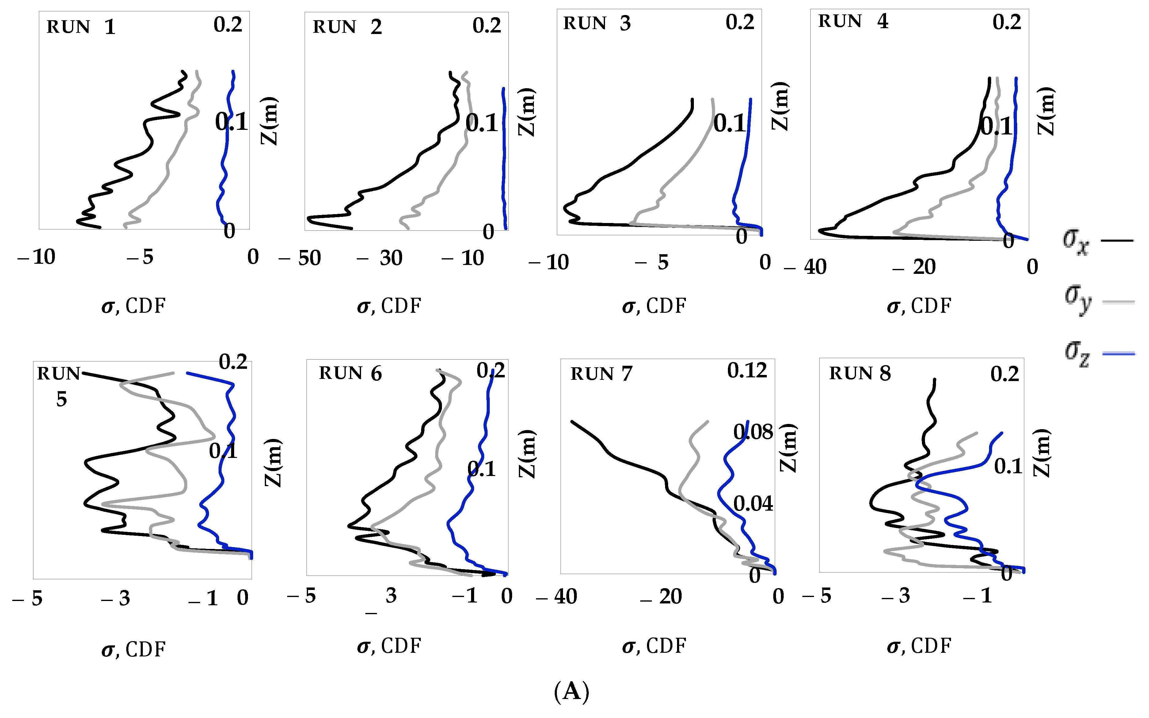
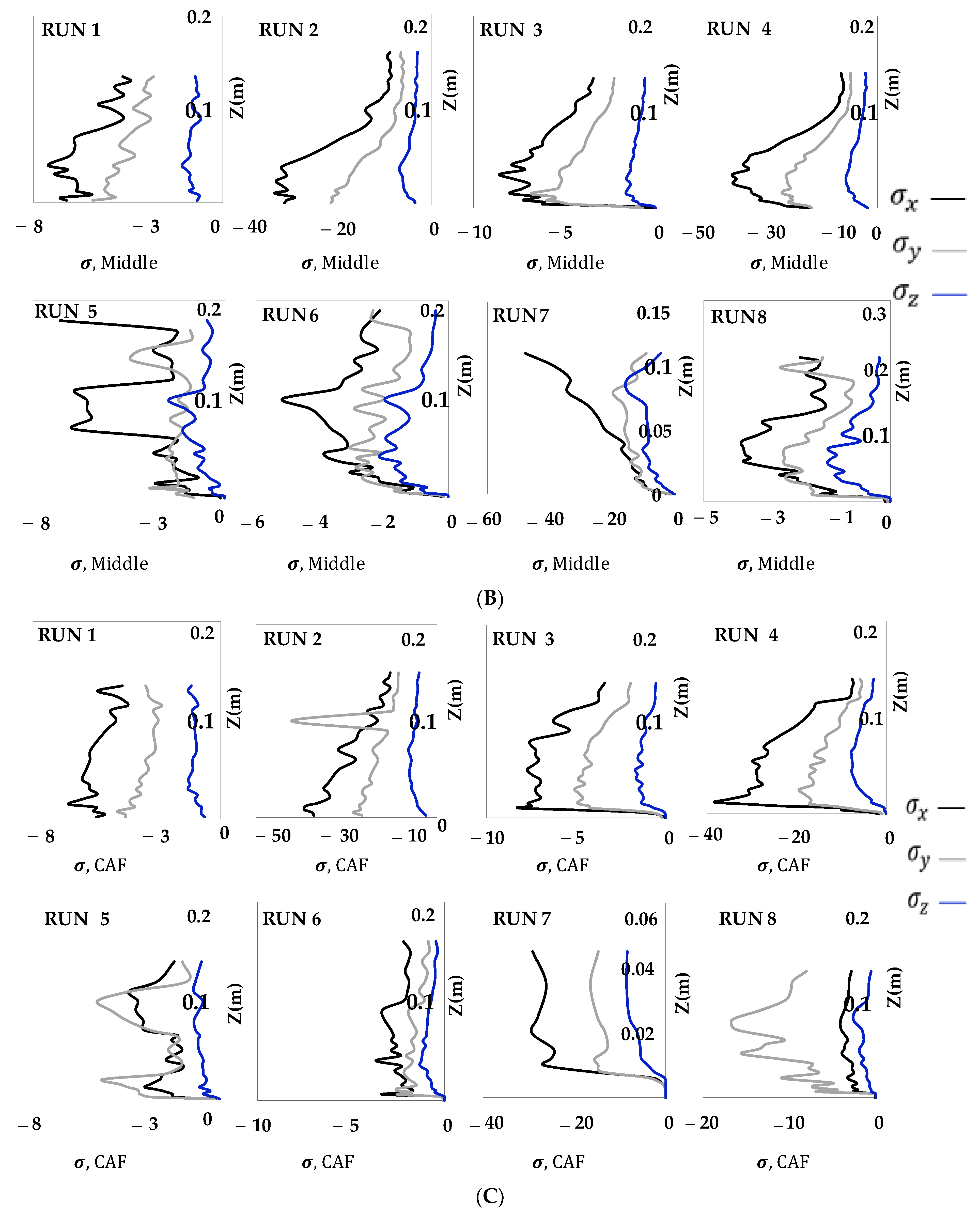
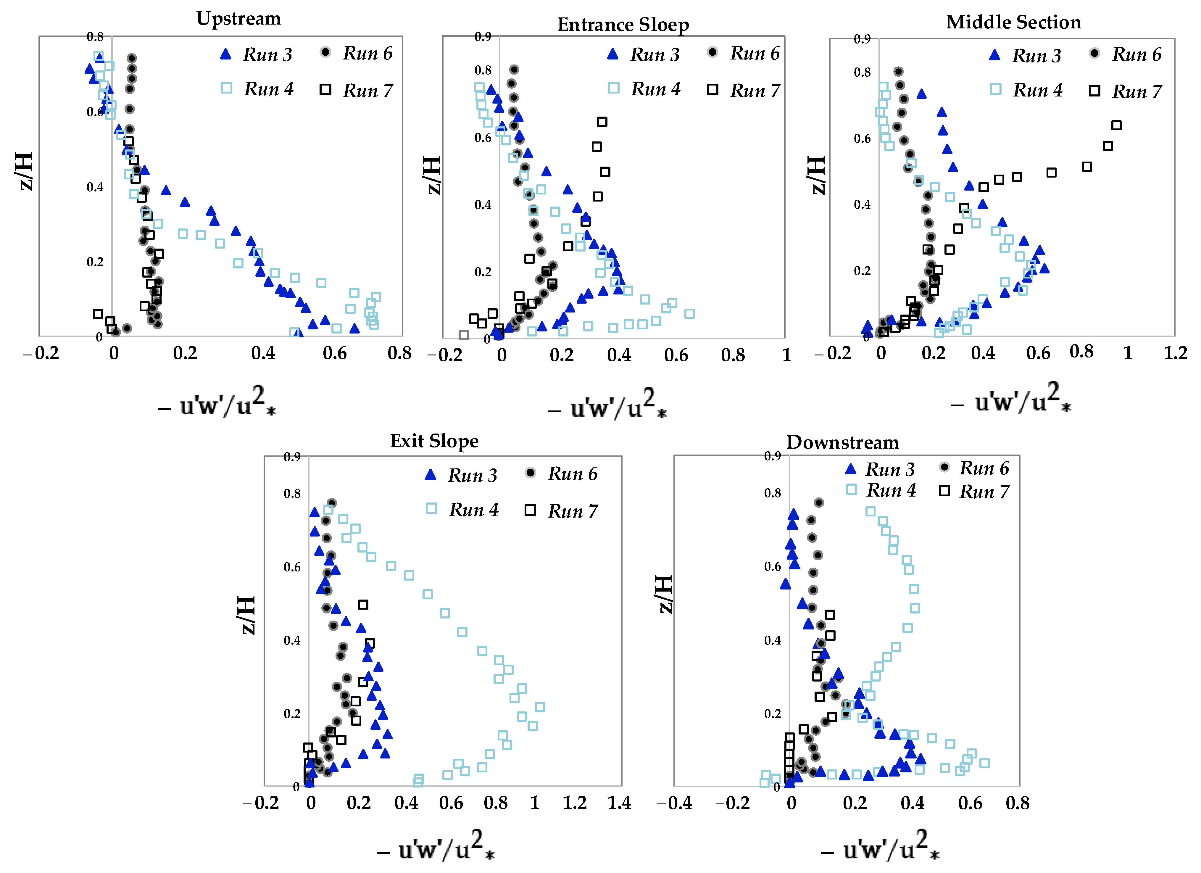
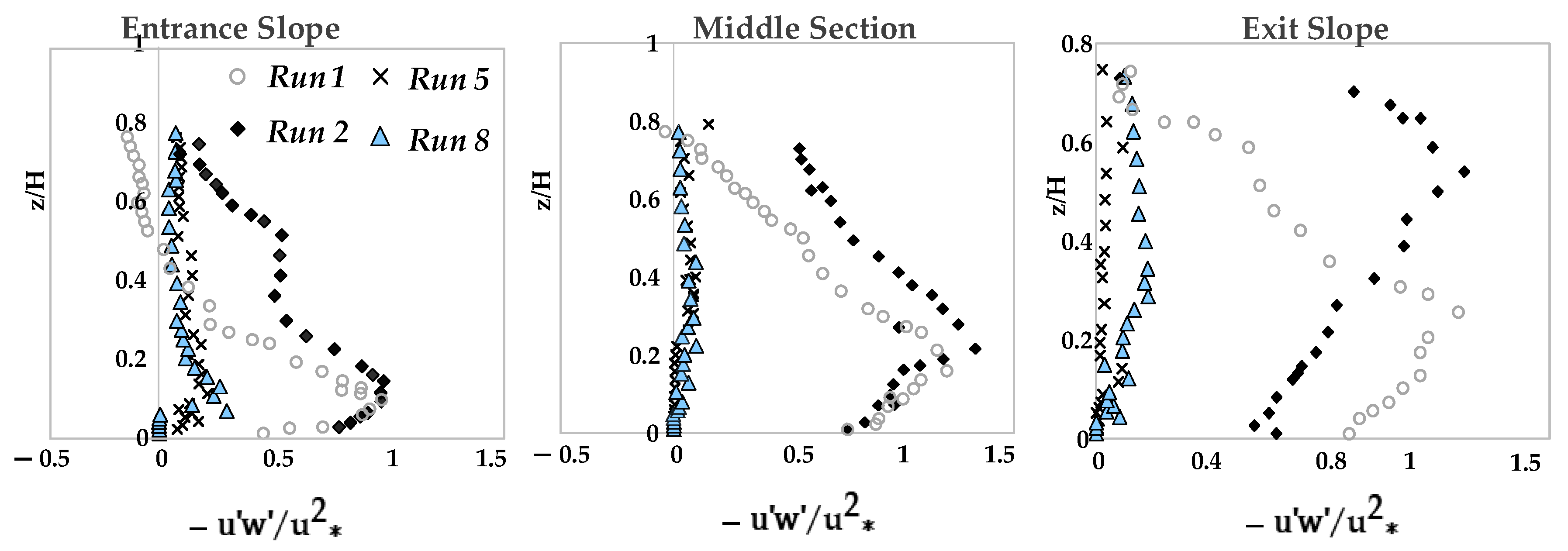
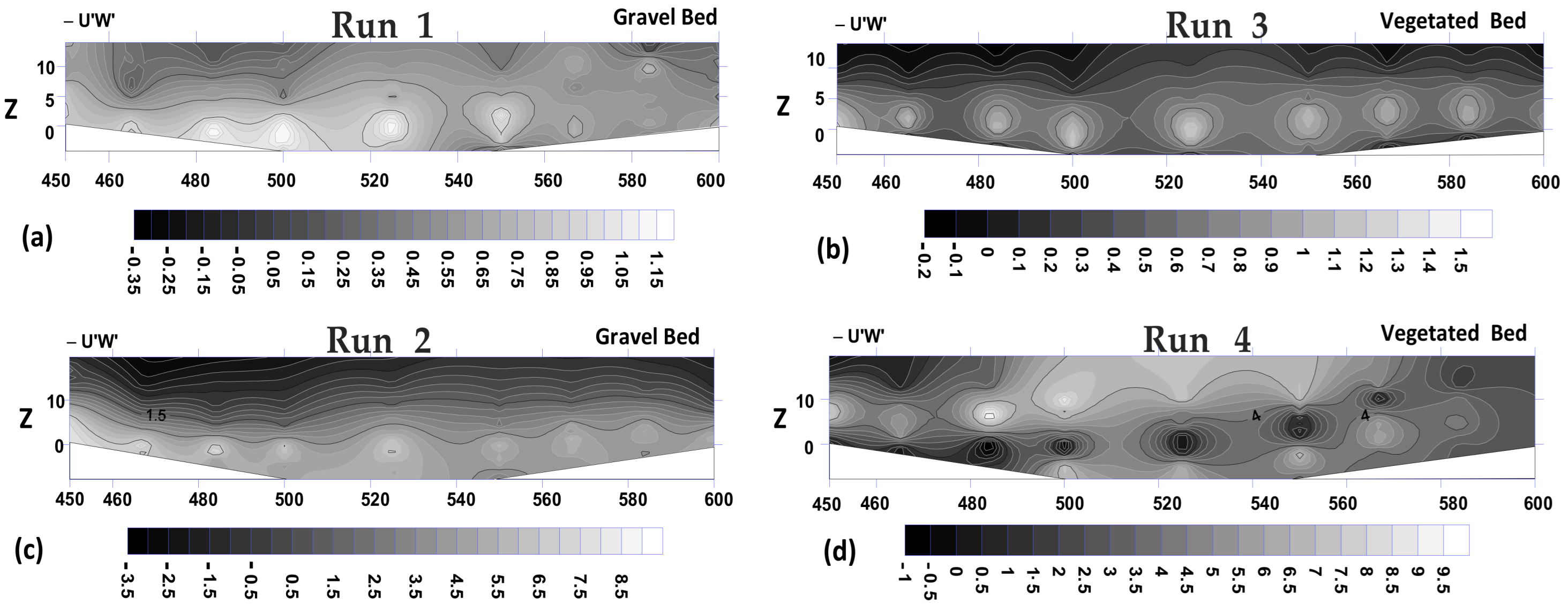
3.2. Reynolds Normal and Shear Stress Distributions

In this study, using the following equation, the dimensional Reynolds normal stresses have been estimated at three locations (entrance slope, middle pool section, and exit slope) along the pool bed, which is depicted in Figure 5.

$${\mathsf{\sigma }}_{\mathrm{x}}=-\mathsf{\rho }\overline{{\mathrm{u}\prime }^2}, {\mathsf{\sigma }}_{\mathrm{y}}=-\mathsf{\rho }\overline{{\mathrm{v}\prime }^2}, {\mathsf{\sigma }}_{\mathrm{z}}=-\mathsf{\rho }\overline{{\mathrm{w}\prime }^2}$$

(1)

Under the condition of a constant flow discharge, the normal stresses on the pool bed with vegetation patch are clearly greater than those on the gravel surface without vegetation (Runs 1 and 3). The magnitude of the normal stress decreases as the flow rate rises (Runs 2 and 4). Moreover, the magnitude of the normal stress decreases as the bed slope decreases (Runs 3 and 6). Additionally, when the aspect ratio rises, the magnitude of the normal stress decreases at the water surface (Run 7). This phenomenon occurs due to the stronger secondary currents in shallow flows (W/h = 2.7). For all experimental runs, the magnitudes of the normal stresses in three directions of the flow are shown in Figure 6A for the entrance slope, for the middle pool section in Figure 6B, and for the exit slope in Figure 6C. The results indicate that the values of the normal stress in most parts of the stream are higher in the stream-wise direction than those in both lateral and vertical directions. However, the magnitude of the normal stress is affected by the presence of secondary currents, resulting in shallow channels with different roughness from the bed (Figure 5). In addition, the Reynolds normal stress distributions are also affected by the bed form slope (Figure 5). This makes it difficult to provide a general pattern for the distribution of the Reynolds normal stress in the bed forms with a vegetation cover.

In Figure 7, Reynolds shear tresses ($-\mathsf{\rho }\overline{\mathrm{u}\prime \mathrm{w}\prime }$) calculated using Equation (2) are normalized with the squared friction velocity ${\mathrm{u}}_{*}^2$, in which ${\mathrm{u}}_{*}$ is the shear velocity calculated from the velocity profiles near the bed, which follows the logarithmic law as presented in Equation (3). Wherein k is the von Karman coefficient, which is equal to 0.41; ${\mathrm{z}}_0$ is the reference bed level that varies with the roughness height of the bed material. In both uniform and non-uniform flows, it has been claimed that the inner zone of each velocity can be extended to a relative depth of z/${\mathrm{z}}_0$ = 0.2 [26].

$$\overline{\mathrm{u}\prime \mathrm{w}\prime }=\frac{1}{\mathrm{N}}{{\displaystyle \sum }}_{\mathrm{i}=1}^{\mathrm{N}}(\mathrm{u}-\overline{\mathrm{u}})\left(\mathrm{w}-\overline{\mathrm{w}}\right)$$

(2)

$$\frac{\mathrm{u}}{{\mathrm{u}}_{*}}=\frac{1}{\mathrm{k}}\ln \frac{\mathrm{z}}{{\mathrm{z}}_0}$$

(3)

In the presence of vegetation canopy in the pool bed, four experimental runs have been conducted. The dimensionless Reynolds shear stress (RSS) profiles are displayed in Figure 7 along the flow direction from upstream to downstream. One can also observe various trends of Reynolds stress for different experimental runs from Figure 7. If the channel bed is smooth, the RSS distribution often shows a linear profile. The rough sub-layer near the bed may cause the Reynolds stress distribution to grow up to 20% of the flow depth before decreasing [22,30,31,32]. Results of the present study indicate that the secondary currents are intensified due to the presence of the vegetation canopy, the non-zero vertical velocities, and the smaller aspect ratio of less than 5. Several researchers have demonstrated that the secondary currents in shallow flows cause the shear stress distribution to deviate from the expected linear shape [6,33].

Depending on the variation in flow velocities, the maximum shear stress can be observed in the upstream portion of the channel, which is located in the zone close to the channel bed within the distance of z/H < 0.15, revealing that the RSS values are completely affected by the roughness elements and relative submergence (H/$d_{50}$) [34]. The positive RSS values close to the water surface support the existence of the dip phenomenon. The greater the slope of the pool entrance section (Runs 6 and 7), the higher the Reynolds stress values are induced along the flow. Furthermore, the shear stress reduced toward the water surface as the flow depth increased, and its distribution profile appeared to have a convex shape. Moreover, the positive pressure gradient (also known as the reverse pressure gradient) and the negative pressure gradient (also known as the favorable pressure gradient) have an impact on the Reynolds stress distribution in the decelerating and accelerating flows, respectively [35].

The shear stress profiles in the middle pool section do not exhibit a tendency toward a linear shape, suggesting that the flow is not homogeneous there. In the presence of a vegetation patch in the pool, the increased flow velocity leads to an increase in the shear stress values in the zone of z/H < 0.2 due to higher turbulence intensities. For all experimental runs, the maximum shear stress inside the middle pool section occurred away from the channel bed depending on the flow velocity and slopes of entrance and exit sections, specifically the maximum RSS is observed at a depth of z/H = 0.25 in the middle part of the flow (Run 3, 4, and 6) [24,36]. However, the impact of secondary currents resulting from the increase in the aspect ratio has the opposite effect on the location of the maximum shear stress and is shifted toward the water surface (Run 7). For the same flow discharge, as the results showed from Runs 3 and 6, with the increase in the slope of the entrance section (namely, with the decrease in flow velocities), the RSS values increased in the zone of z/H < 0.5 (except for the middle pool section).

Due to significant disturbances resulting from bed forms and roughness, the shape of shear stress distribution profiles in the downstream section of the pool differs from that in the upstream section of the pool. Negative Reynolds stresses are also observed sometimes, as illustrated in Figure 7. Most likely, this results from the flow being transmitted to each component’s wake zone by vegetation-induced drag. Nonetheless, the previous investigations in the presence of vegetation and bed morphologies also reported the existence of negative RSS values. These results demonstrated that, even if the sweep and ejection events result in positive RSS values in the flow field, the outward and inward events in the bursting process might be responsible for the negative stresses.

In some places, particularly in the zones where the flow was accelerating, the RSS value increased dramatically. It may be explained by the fact that when the flow is accelerated, or even when the channel bed has a larger slope, the turbulent velocity components undergo some changes, as indicated in Figure 7 and Figure 8. Moreover, the distribution of the flow responds more strongly and quickly to the changes in the bed slope near the channel’s side walls than it does near the channel’s centerline (Figure 8). It has been observed from Figure 9 that, over the gravel pool bed, the highest Reynolds stress region grows to the end of the middle pool section. Figure 8 also demonstrates this result for flow over a gravel bed form, as the maximum RSS is highest along the middle and exit sections of the pool. However, with a lower flow discharge, the presence of vegetation resulted in an obvious decrease in the shear stress (Run 3). While with the higher flow discharge, the vegetated canopy minimizes shear stresses on the entrance slope, the zone with the greatest stress is only visible in the middle section of the pool bed (Run 4).

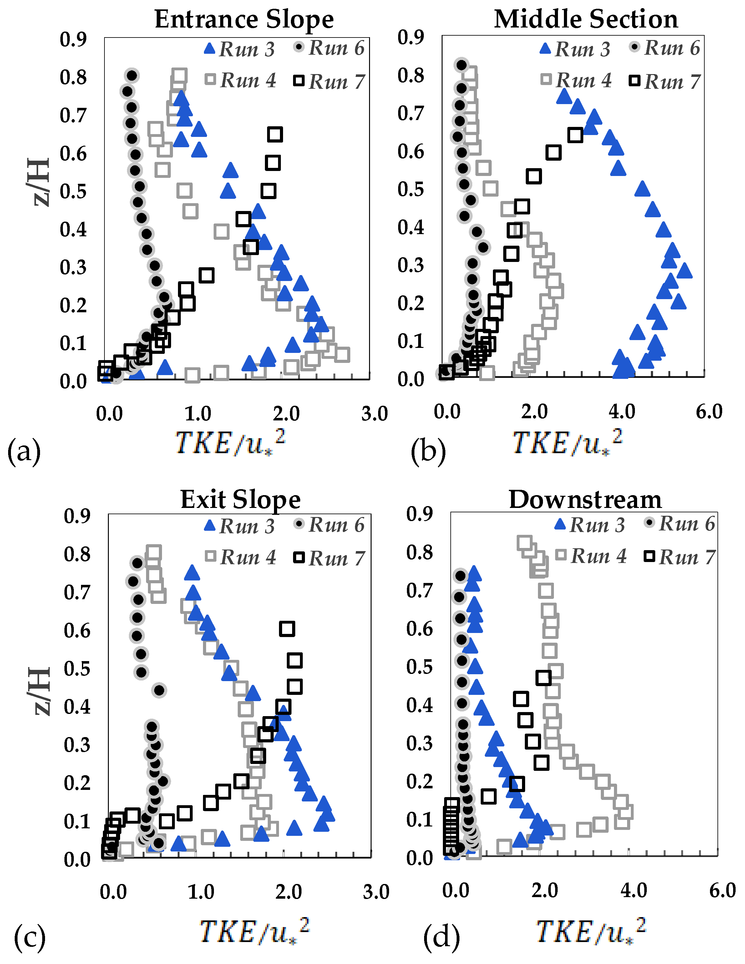
3.3. Turbulence Kinetic Energy (TKE)

As seen in Figure 3, the velocity profile in the inner layer of the flow is almost constant due to the significant wake effects resulting from the vegetation canopy; this zone exhibits negligibly little vertical momentum transmission, although it may occasionally appear with a slight contour gradient. Similar to the results reported by the previous researchers regarding open-channel flow in the presence of either emergent or submerged vegetation, this inner layer zone refers to the “longitudinal exchange zone”, which has a negligibly limited vertical momentum conveyance [37,38,39]. The logarithmic law is used to describe the turbulence structure in this zone. Figure 10 represents the variation of the dissipation rate of turbulent kinetic energy (TKE = $0.5c_2\rho \left[\overline{{\mathrm{u}}^{\prime 2}}+\overline{{\mathrm{v}}^{\prime 2}}+\overline{\mathrm{w}{\prime }^2}\right]$), normalized with the squared friction velocity $\left({\mathrm{u}}_{*}{}^2\right)$, with respect to flow depth in central pool section where vegetation patch presents. In the mixing layer (as shown in Figure 11), due to the vertical transfer of momentum, the unstable inflection point of velocity is induced by secondary currents. Moreover, in the mixing layer of flow at the canopy part, the turbulent diffusion has an obvious impact on the turbulence kinetic energy (TKE) budget.

Figure 10 shows that the great TKE values are observed at different locations in several flow sections. The energy losses are reduced; i.e., as the entrance slope increases, the pressure losses per unit length of the bed are reduced, leading to lower RSS values [17]. In fact, the mixing eddies resulting from the velocity gradient over the vegetation canopy decreased, and the reduction in the entrance slope of a pool led to the turbulence becoming weaker. The profiles of TKE for Run 7 values do not follow a convex shape, as they indicate the higher entrance and exit slopes, justifying the significant role of bed-form geometry on the TKE distribution. In addition, due to the stronger secondary currents and higher turbulence velocity, an increase in flow velocity by reducing flow depth resulted in larger TKE values in Run 7.

The maximum TKE value is predicted to occur generally in a zone that is relatively close to the bed (z/h < 0.2) since the production of Von Karman vortexes is typically associated with the occurrence of TKE values that peak a severe distortion in the velocity profile [9]. Moreover, other studies have revealed lower ranges for the wake zone in streams with broad and heavily submerged vegetation as well as in streams with broad, partially submerged vegetation in the bed. Results of the present study support the existence of a small wake zone over the vegetation canopy [2,13] only for the small bed-form slopes (Runs 3 and 4).

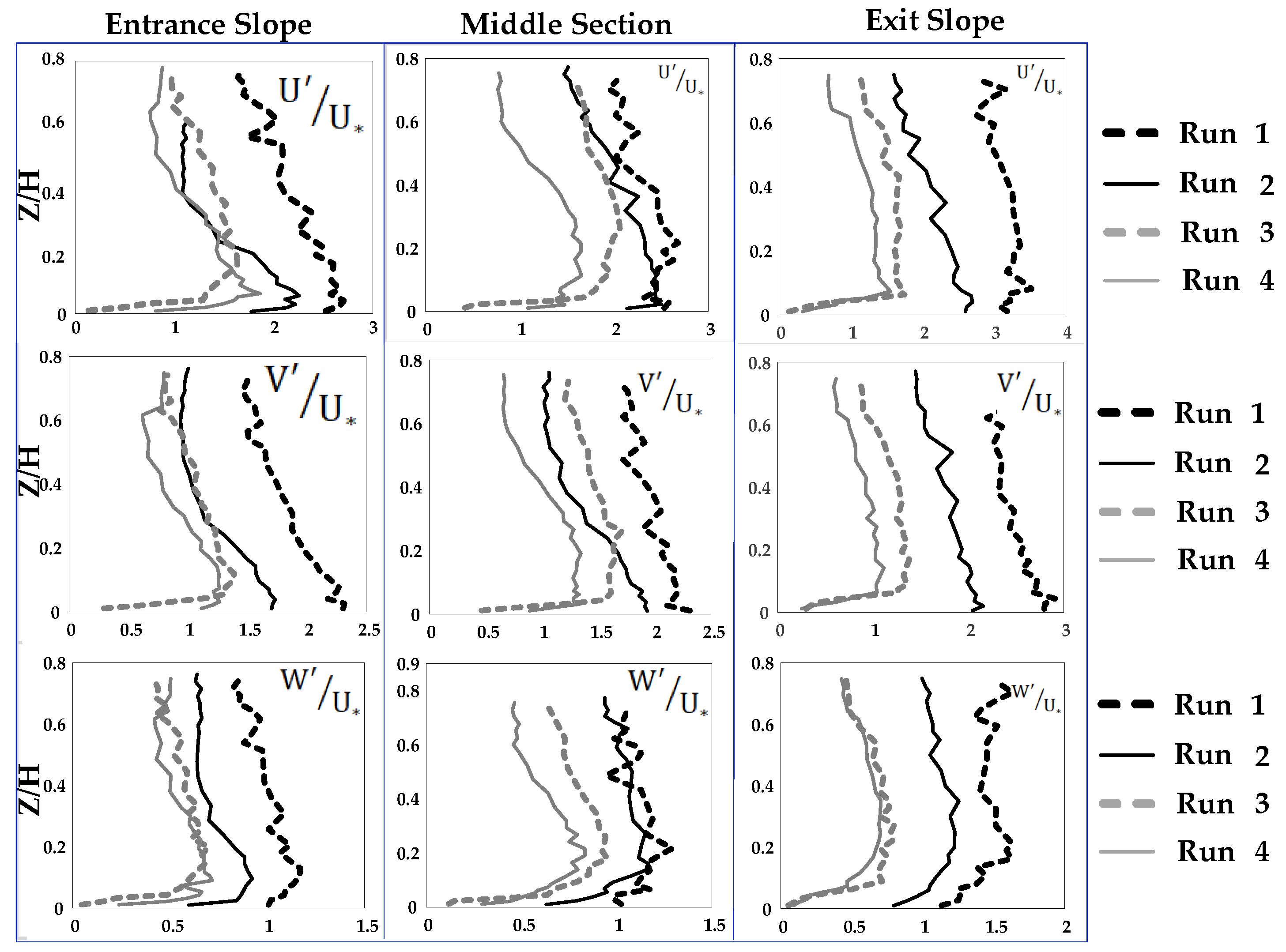
3.4. Turbulence Intensities

By calculating the root mean square (RMS) of flow velocities, turbulence intensity is displayed in Figure 12 to show the values of intensities for pool setup 1. It has been found that the vertical turbulence intensity is highest in the upper layer above the canopy of vegetation, about in the zone of z/H < 0.2, while stream-wise and lateral turbulence intensities reach their maximum slightly above the canopy of vegetation.

Research results showed that the maximum intensity of the streamwise turbulence (u’) occurs right above the canopy, while the maximum intensity of the vertical turbulence occurs right below the emergent canopy. Due to the non-uniformity of flow in experiments, the values of u’, in particular, exhibit a convex shape rather than a concave one, which deviates from the exponential law proposed by Nezu [38]. This suggests that vegetation considerably modifies the equilibrium state of turbulent kinetic energy and, thus, the redistribution of turbulence intensities. In fact, it should be noted that the isotropic turbulence inside vegetation (including the vegetation stems and canopy) occurs when there is a strong wake of turbulence over those objects. As a result, the wake caused by vegetation elements may cause convex patterns of turbulence intensities in a cascade process [31]. Similar convex-shaped distribution of turbulence intensity has been reported in studies of the aquatic canopies [39].

It appears that the presence of vegetation has a considerable impact on the kinetic energy and the distribution of turbulence intensities [17,40]. Figure 12 displays the possible relationship between the highest disturbance intensity and the bed slope of the flume. Along the accelerating part of the flow, the value of disturbance over the gravel bed form is larger than the values recorded in the decelerating region. Streams with vegetation patches, on the other hand, did not exhibit the same pattern.

The maximum amount of disturbance over the gravel bed form along the accelerating section of the flow has greater values than that along the decelerating section. However, streams with vegetation patches did not show a similar trend. The turbulence intensities over the decelerating and accelerating sections did not have a significant difference.

The zone of the inner layer with the largest turbulence intensities can be seen around the zone of z/H < 0.2, while in the central region of the flow, it appeared to be in the zone of z/H < 0.4. These zones (or flow depths) are also thought to be the spots where shear stress is at its highest. Instead of the accelerating flow, the decelerating flow intensifies the turbulence and increases Reynolds shear stress, indicating that flow structures are affected by the non-uniformity of the flow [6,32,41].

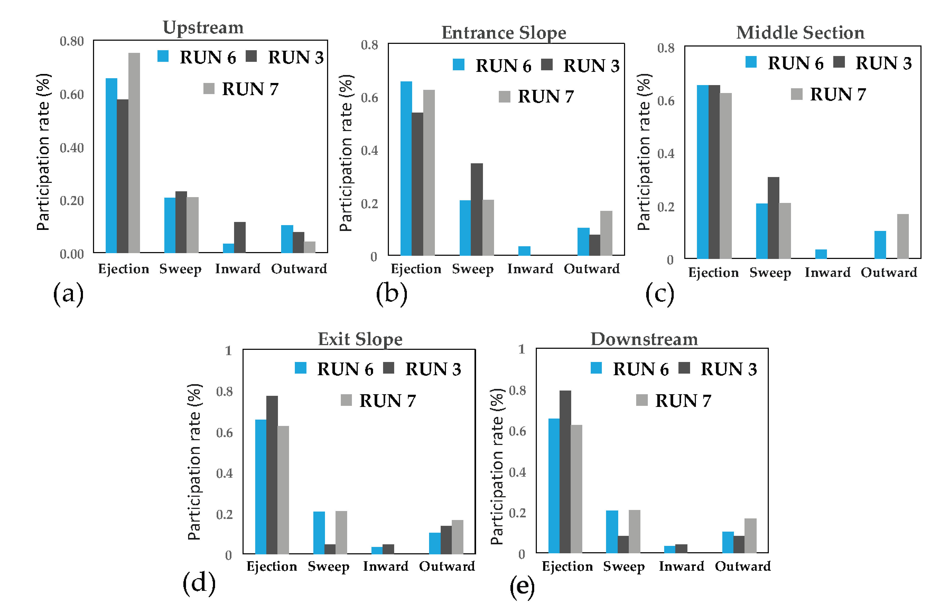
3.5. Quadrant Analysis

A quadrant analysis has been applied to predict detailed statistical characteristics of turbulent flow structures [42,43]. However, to the authors’ knowledge, no study has been reported on the quadrant analysis of flow structure at the trailing edge of a vegetation patch in a gravel-bed stream. This study focuses on the exit border of flow from the vegetation patch in a gravel-bed channel. The important question is, what happens for turbulent flow structures at the trailing edge of a vegetation patch over a pool, and how does it affect the estimations of hydraulic parameters in this study?

As mentioned by Parvizi et al. [35], the outward motion of the flow is a result of the positive values of u’ and v’ in bursting process occurrences; the sweep motion is recognized with the positive value of u’, and the negative value w’ generally corresponds to the flow stream over the vegetation canopy (often denotes the flow stream above the vegetation canopy). However, the ejection motion of the bursting phenomenon, which has a positive value for w’ and a negative value for u’, along with the sweep motion, have been observed over smooth walls in the boundary layer [42,43]. Lastly, the flow has been recognized to be moving inward if both u’ and w’ have negative values. The presence of vegetation patches over the bed form plays a role in the flow structure. However, this aspect of fluvial hydraulics has been considered less often by researchers. This part of the study especially concentrates on the border between vegetation and grave. The important question is, what happens in the trailing edge of a vegetation patch over a pool, and how does this affect the turbulence features and their distributions? It appears that the sweep motion is the primary event of the flow downstream of the pool (trailing edge of a vegetation patch), where the flow reaches the gravel bed again. Nonetheless, according to the result of experiment Run 7, the isotropic event often occurs near the boundary between the vegetation patch and gravel bed (trailing edge of the vegetation patch). The contribution of each quadrant event is presented in Figure 13, indicating the dominant role of the ejection motion in the bursting process of the flow and the sweep motion as the second dominant event in the stream.

Along the decelerating part of the flow (CDF), sweep motion appears above the vegetation canopy in the inner layer of the flow in the zone of z/H < 0.2, while the modification of the entrance slope doesn’t lead to the change of the zone for the occurrence of the sweep motion in the stream (Runs 3 and 6). However, by adjusting the aspect ratio in the flow (Run 7, from w/H = 2.0 to 2.7; w/H < 5.0), the sweep phenomenon has been seen in a higher layer of the stream in the zone of z/H < 0.5, indicating that the change of flow velocity results in the occurrences of bursting events. By increasing the slope of the entrance section of the pool, a larger region for the sweep phenomenon resulted, while a higher sweep zone (z/H < 0.4) was observed by altering the aspect ratio. The sweep motion has been noticed right above the vegetation canopy in the acceleration section of the flow. However, a larger zone of sweep motion has been generated because of the modification of the slope of the exit section of the pool. In addition, Figure 13 shows that the ejection motion is the primary event of the flow at the trailing edge of vegetation.

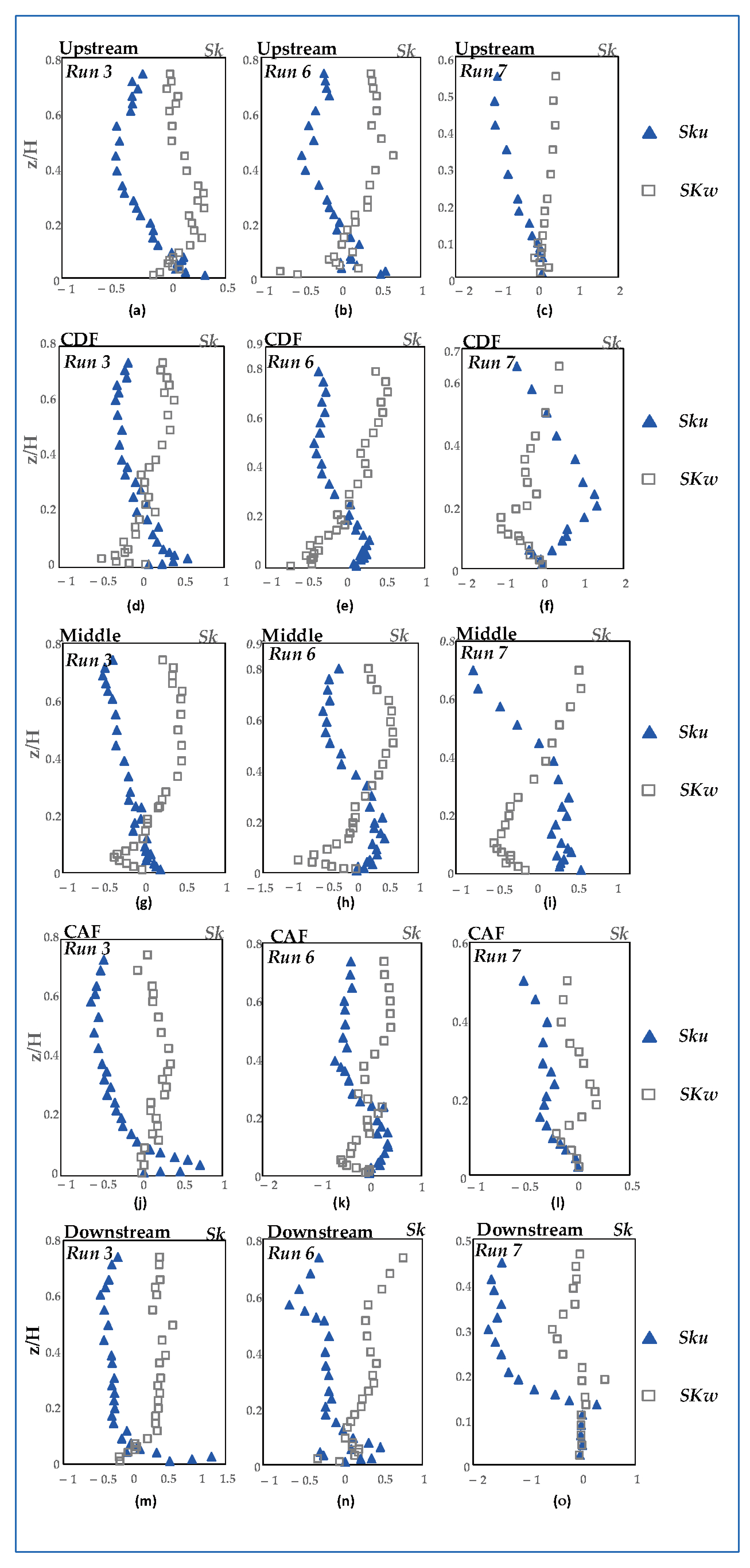
3.6. Skewness Coefficients

Skewness coefficients (${\mathrm{sk}}_{\mathrm{u}}$ and ${\mathrm{sk}}_{\mathrm{w}}$) of velocity fluctuations are the third central moment of the factors u’ and w’, which include positive, negative, or zero values in turbulent flows. Asymmetry in a flow field can be better understood by looking at the skewness factors [18]. Positive skewness means that the variable u’ is more likely to take on a large positive value than a large negative one. In fact, a non-zero skewness of velocity fluctuations in the stream-wise and vertical directions indicates an asymmetric probability density function (PDF) of the considered variable, namely, the dominated processes in one direction are more possible than in the other one depending on the symptom of the statistics.

The positive skewness indicates that the PDF has a longer tail for u’ > 0 than that for u’ < 0. A zero-skewness value shows an isotropic or homogenous turbulence. The possible explanation is that instability of the inflection point of velocity profiles is responsible for the generation of coherent eddies in the presence of flexible vegetation inflows. This implies that coherent eddies, such as ejections and sweeps, will resonate with the flexible vegetation [35].

Figure 14 displays the skewness for measured velocity fluctuations (${\mathrm{sk}}_{\mathrm{u}}$ and ${\mathrm{sk}}_{\mathrm{w}}$) from experiments based on data collected from experimental Runs 3, 6, and 7 along the upstream, entrance slope with a decelerating flow (CDF), middle-pool section, and exit sections which leads to an accelerating flow (CAF) of the pool while maintaining the same flow rate and vegetation canopy. The sweep motion is the major event right above the gravel grains in the zone of z/H < 0.1 in the upstream region of the pool, where the fluctuations of flow velocity mostly depend on two parameters, flow depth (H), and median grain size of bed material (${\mathrm{d}}_{50}$) (Runs 3 and 6). To precisely study flow dynamics, data was collected at the boundary of the gravel bed and vegetation patch at the upstream portion of the pool, as shown in Figure 13c.

One can see from Figure 14 that ${\mathrm{sk}}_{\mathrm{u}}$ has slightly positive values at point c together with a positive ${\mathrm{sk}}_{\mathrm{w}}$ values, where vegetation patch begins at the gravel border, implying that the outward motion has occurred closely above the gravel barrier in the zone of z/H < 0.1.

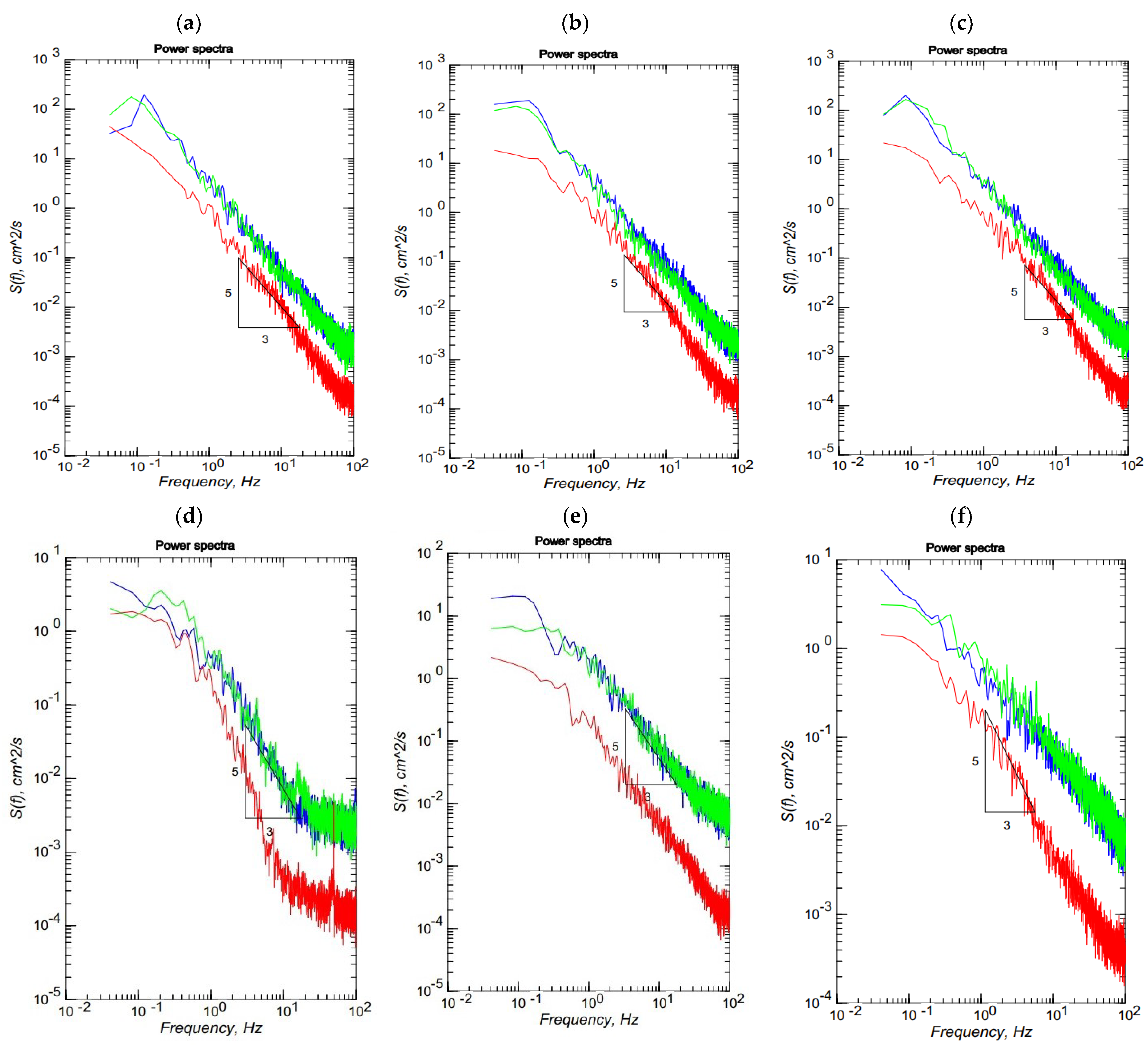
3.7. Spectral Analysis

There are three distinct scaling regimes observed in turbulent flows across flat surfaces. At low frequencies, there is a scaling sub-range, which is referred to as the production subrange, characterized by a −1 spectral slope. At intermediate frequencies, Kolmogorov claimed that an inertial subrange with a spectral slope of −5/3 is seen. When the Reynolds number is high enough, Kolmogorov claims [40] that there is no loss of energy during the shift from large to tiny eddies scale. The third scaling subrange is the viscous subrange, where spectra decay significantly faster than in the inertial subrange [41]. It is expected that the presence of topography and bed forms in the regimes both affect the transition of eddies between the production and inertial subranges [42].

Spectral analysis has been performed for velocity components along the bed form at the same points located at 6 mm from the vegetation cover along the entrance slope, middle pool section, and exit slope of the pool. The “6 mm” was selected because this is almost the closest point to the bed where the ADV can collect data without any difficulty. Moreover, the distance of 6 mm from the vegetation cover is selected in this study to compare the results of this study to those of other studies, such as Najafabadi et al. [43].

The power spectral densities of velocity components in Figure 15 are presented for three velocity components; stream-wise velocity is presented as blue curves; spanwise velocity components are presented as green curves, and vertical velocity components as red curves. Figure 15 shows a slight deviation in Kolmogorov’s −5/3 power law for the vertical velocity component from the inertial subrange with the presence of a smaller bed slope, but it is generally valid (Figure 15a–c). The slight deviation resulted from the vegetation on the bed limiting its effect to near the vegetation. In addition, the Kolmogorov scale may mainly represent a balance between the kinetic and viscous energy in the flow field and not necessarily an eddy scale, which could explain this discrepancy in the velocity deviation of the Kolmogorov law.

Najafabadi et al. (2018) reported that Kolmogorov’s −5/3 power law is prominent only at the deepest point of the bed form [43]. However, the result of the present study shows that the law rests universally for the trailing edge of the vegetation patch in the 3D bed form, as it is reported for the 2D pool with the 3D flow in a laboratory experiment over the gravel bed [44,45]. Figure 15 shows that the shedding frequency falls between 1.8 and 4.0 Hz. However, Nepf (1999) reported that this range is (1.8–3.6 Hz) for a random cylinder as emergent vegetation [46], but (1.0–1.8 Hz), as reported by Lacy and Roy (2007) [47]. Over the gravel bed between vegetation patches, Afzalimehr et al. (2021) pointed out that this range is from 3.0 to 7.7 Hz [48]. This comparison shows that the shedding frequency is affected by the changes in the bed-form slope as well as the presence of 3D bed forms and vegetation patches, resulting in higher values than those reported in the literature [49].

4. Discussions

In this section, a comparison of the results of this study to those of Nepf and Ghisalberti (2008) [4] and Wang et al. (2022) [42] has been presented in order to clarify the contribution of the present research. In the study of Nepf and Ghisalberti (2008) [4], they did not consider the effect of the 3D bed forms and a dense vegetation patch without flexibility, but they considered plant stems as rigid circular cylinders with a specific distance between the rigid circular cylinders. Thus, the turbulent structure in their study is completely different from that of the present study. Nepf and Ghisalberti (2008) [4] could investigate the flow structures inside the vegetation patch because the setup of vegetation stems was spaced apart, and this type of setting enabled them to collect data inside the vegetation patch using an ADV. A comparison of Reynolds stress (RS) distribution reported by Nepf and Ghisalberti (2008) [4] and that of the present study shows that the location of the bed form (entrance, middle, and exit sections) plays a significant role in the RS distribution and, thus, leads to different results. For example, the Reynolds stress distribution (Figure 5 in the study of Nepf and Ghisalberti (2008) [4]) displays a clear convex distribution. In the present study, however, the RS distribution is affected by the entrance slope of the pool and vegetation cover. As shown in some profiles, the negative RS values are due to the different contributions of bursting events and the role of the 3D bed form in the generation of secondary currents. In some runs (Run 7 in the middle pool section of Figure 7), the RS has an increasing trend rather than a decreasing trend toward the water surface. Their objective was to investigate the RS distribution and to identify the effect of vegetation deflection on creating a smaller vegetation height under stronger flow conditions [4]. In this study, it is emphasized that data are unable to collect inside the vegetation patch due to a very thin vegetation layer (the height of vegetation is only 2 cm) and no change in vegetation flexibility. However, Nepf and Ghisalberti (2008) [4] investigated flexible canopies, where the passage of the Kelvin–Helmholtz vortices generated a wave called Monami, showing a progressive wave along the canopy interface. Furthermore, they reported that the stem geometry played a significant role in turbulent flow structures. In the present study, we investigated the interaction of vegetation cover without rigid stems and with no flexibility at some important locations, such as the trailing edge of the vegetation patch. The results of this study indicate that the application of the specific (constant) values of velocity and Reynolds stress for all parts of a bed form will lead to incorrect estimation of hydraulic parameters (e.g., resistance).

Wang et al. (2022) [42] compared the influences of flexible vegetation on the flow velocity to those of rigid vegetation and found that the vegetation tilt has little effect on the difference between flow velocity inside the vegetation and that of vegetation canopy as well as the turbulence structure in the flow. However, the present study does not consider velocity structure inside the thin vegetation layer. The results of this study indicate that the bed-form slopes (entrance and exit sections), vegetation patches, and the location of the pool (entrance, middle, and exit sections) affect the velocity distribution. Results of the spectral analysis show that Kolomogrove −5/3 law over the 3D vegetation patch rests valid as it does for the 2D pools and 3D flows. Wang et al. (2022) [42] used a flatbed with vegetation with the height of 0.2 and 0.1 m and arranged vegetation elements in five rows in the streamwise direction and nine rows in the spanwise direction (there is a distance between pellets), where the flow passed through the vegetation patch. By comparing the TKE values in the flow with inclined rigid vegetation to those with vertical rigid vegetation, they found that the TKE in the former case was obviously smaller than that with vertical rigid vegetation. Wang et al. (2022) [42] investigated the energy spectra at the height of the vegetation canopy directly above a row of plants and in the middle of the two rows of plants. They reported that Kolmogorov’s −5/3 scaling law is satisfied in the inertial subrange of flow with rigid vegetation. However, they haven’t investigated the validation of this law at the trailing edge of the 3D vegetation patch.

5. Conclusions

The flow in any rivers in arid and semi-arid regions decreases dramatically during summer. As a consequence, vegetation patches develop in different parts of the rivers. When the water level increases in these rivers during spring, fall, and winter, the hydraulic conditions in rivers with the presence of vegetation patches are completely different from those without vegetation. Thus, some hydraulic parameters, including flow velocity and Reynolds stress, can be over- or underestimated due to the presence of the vegetation patches in channels. To better understand the changes in hydraulic parameters along 3D vegetation patches, experiments have been carried out in a laboratory flume with an artificial bed form. Two slopes of 5 and 10 degrees for both the entrance and exit sections of the pools have been utilized. The following results have been drawn with respect to the distribution of velocity profiles, Reynolds normal and shear stresses, TKE, turbulence intensities, skewness coefficients, and bursting process:

(1)

In general, the bed-form slopes of both entrance and exit sections, the vegetation patches, and the location of the pool (entrance, middle pool, and exit section) affect the velocity profile, Reynolds shear stresses, TKE distribution, and the contribution of each bursting events on the turbulent flow structures. For a pool with entrance and exit slopes of 10 degrees, the TKE distribution has no specific form (Run 7). However, for a pool with a small entrance and exit slope of 5 degrees (Runs 3 and 4), the TKE distribution has a convex shape with the maximum value near the bed. Results of the quadrant analysis reveal that the bursting events at the trailing edge of the vegetation patch, where the flow exits from the vegetation patch to the gravel bed, display different distributions compared to other locations along the 3D vegetation patch. This difference plays a significant role in estimating flow resistance in open channels. The validation of the spectral analysis of the Kolmogorov power law for different bed-form slopes has been conducted;

(2)

The Reynolds normal stress in the stream-wise direction is greater than those in both lateral and vertical directions. There is a disruption of normal stress values in the stream-wise direction due to the presence of secondary currents generated due to the different roughness of the channel bed and sidewalls of the flume. Therefore, the difference in the roughness and bed slope influences the normal Reynolds stress distributions. In the stream-wise direction, the region with the highest Reynolds shear stress (RSS) moves away from the bed. The RSS values in the zone of z/H > 0.5 decrease as the bed slope increases. A decrease in the reverse pressure gradient and the favorable pressure gradient affects the distribution of Reynolds stresses in both decelerating flow zone (entrance section of a pool) and the accelerating flow zone (exit section of a pool). When the entrance slope of the pool is smaller, the distribution of Reynolds stress is more regular toward the water surface;

(3)

The quadrant analysis in this study focuses on the role of different bursting events at the trailing edge of the vegetation patch where the flow leaves the vegetation patch to the gravel bed. The results of this study clarified that both ejections and sweeps govern the turbulence structures and coherent motions at the trailing edge of the vegetation patch. The presence of the vegetation patch, as well as the changes of both the entrance and exit slopes of a pool, generate the non-uniformity of the flow and increase the turbulence intensity and TKE in the downstream section of the vegetation patch. The sweep motion occurs in a narrower zone above the vegetation canopy. The sweep motions of bursting events are the dominant processes directly above the vegetation canopy, while the outward motion with slightly positive values has been observed at the front edge of the vegetation patch;

(4)

The Kolmogorov −5/3 power law rests valid for the 3D vegetation patch. The geometry of the bed form, including both entrance and exit slopes of a pool, does not influence this law compared to the presence of a vegetation patch in a flat bed;

(5)

The shedding frequency is affected by the changes in the bed-form slopes and the presence of vegetation, resulting in higher values than those reported in the literature.

References

1. Graf, W.H.; Altinakar, M.S. Fluvial Hydraulics: Flow and Transport Processes in Channels of Simple Geometry; Wiley & Sons: New York, NY, USA, 1998. [Google Scholar]
2. Nepf, H.M. Hydrodynamics of vegetated channels. J. Hydraul. Res. 2012, 50, 262–279. [Google Scholar] [CrossRef] [Green Version]
3. Dey, S. Fluvial Hydrodynamics, Hydrodynamic and Sediment Transport Phenomena; Springer: Berlin/Heidelberg, Germany, 2014. [Google Scholar]
4. Nepf, H.; Ghisalberti, M. Flow and transport in channels with submerged vegetation. Acta Geophys. 2008, 56, 753–777. [Google Scholar] [CrossRef]
5. Shi, H.; Zhang, J.; Huai, W. Experimental study on velocity distributions, secondary currents, and coherent structures in open channel flow with submerged riparian vegetation. Adv. Water Resour. 2023, 173, 104406. [Google Scholar] [CrossRef]
6. MacVicar, B.J.; Rennie, C.D. Flow and turbulence redistribution in a straight artificial pool. Water Resour. Res. 2012, 48, W02503. [Google Scholar] [CrossRef]
7. Sawyer, A.M.; Pasternack, G.B.; Moir, H.J.; Fulton, A.A. Riffle-pool maintenance and flow convergence routing observed on a large gravel-bed river. Geomorphology 2010, 114, 143–160. [Google Scholar] [CrossRef]
8. Thompson, D.M. The role of vortex shedding in the scour of pools. Adv. Water Resour. 2006, 29, 121–129. [Google Scholar] [CrossRef]
9. Huai, W.-X.; Zhang, J.; Wang, W.-J.; Katul, G.G. Turbulence structure in open channel flow with partially covered artificial emergent vegetation. J. Hydrol. 2019, 573, 180–193. [Google Scholar] [CrossRef]
10. Tang, C.; Yi, Y.; Jia, W.; Zhang, S. Velocity and turbulence evolution in a flexible vegetation canopy in open channel flows. J. Clean. Prod. 2020, 270, 122543. [Google Scholar] [CrossRef]
11. Ortiz, A.C.; Ashton, A.; Nepf, H. Mean and turbulent velocity fields near rigid and flexible plants and the implications for deposition. J. Geophys. Res. Earth Surf. 2013, 118, 2585–2599. [Google Scholar] [CrossRef]
12. Zong, L.; Nepf, H. Vortex development behind a finite porous obstruction in a channel. J. Fluid Mech. 2012, 691, 368–391. [Google Scholar] [CrossRef]
13. Liu, C.; Hu, Z.; Lei, J.; Nepf, H. Vortex Structure and Sediment Deposition in the Wake behind a Finite Patch of Model Submerged Vegetation. J. Hydraul. Eng. 2018, 144, 04017065. [Google Scholar] [CrossRef]
14. Raupach, M.R.; Finnigan, J.J.; Brunei, Y. Coherent eddies and turbulence in vegetation canopies: The mixing-layer analogy. Boundary Layer Meteorol. 1996, 78, 351–382. [Google Scholar] [CrossRef]
15. Okamoto, T.-A.; Nezu, I. Spatial evolution of coherent motions in finite-length vegetation patch flow. Environ. Fluid Mech. 2013, 13, 417–434. [Google Scholar] [CrossRef]
16. Houra, T.; Tsuji, T.; Nagano, Y. Effects of adverse pressure gradient on quasi-coherent structures in turbulent boundary layer. Int. J. Heat Fluid Flow 2000, 21, 304–311. [Google Scholar] [CrossRef]
17. Ghisalberti, M.; Nepf, H.M. Mixing layers and coherent structures in vegetated aquatic flows. J. Geophys. Res. 2002, 107, 3-1–3-11. [Google Scholar]
18. Kumar, P.; Sharma, A. Experimental investigation of 3D flow properties around emergent rigid vegetation. Ecohydrology 2022, 15, e2474. [Google Scholar] [CrossRef]
19. Kazem, M.; Afzalimehr, H.; Sui, J. Characteristics of Turbulence in the Downstream Region of a Vegetation Patch. Water 2021, 13, 3468. [Google Scholar] [CrossRef]
20. Liu, M.; Huai, W.; Ji, B. Characteristics of the flow structures through and around a submerged canopy patch. Phys. Fluids 2021, 33, 035144. [Google Scholar] [CrossRef]
21. Bassey, O.B.; Agunwamba, J. Derived Models for the Prediction of Cole’s and Dip Parameters for Velocity Gradients Determination in Open Natural Channels. J. Civ. Environ. Res. 1998, 8, 1–19. [Google Scholar]
22. Kironoto, B.; Graf, W.H.; Reynolds. Turbulence characteristics in rough uniform open-channel flow. Proc. ICE Civ. Eng. Mar. Energy 1994, 106, 333–344. [Google Scholar]
23. Dey, S.; Nath, T.K. Turbulence Characteristics in Flows Subjected to Boundary Injection and Suction. J. Eng. Mech. 2010, 136, 877–888. [Google Scholar] [CrossRef]
24. Afzalimehr, H.; Nosrati, K.; Kazem, M. Resistance to Flow in a Cobble-Gravel Bed River with Irregular Vegetation Patches and Pool-Riffle Bedforms (Case study: Padena Marbor River). Ferdowsi Civ. Eng. JFCEI 2021, 2, 35–50. [Google Scholar]
25. Song, T.; Chiew, Y.M. Turbulence Measurement in Nonuniform Open-Channel Flow Using Acoustic Doppler Velocimeter (ADV). J. Eng. Mech. 2001, 127, 219–232. [Google Scholar] [CrossRef]
26. Coles, D. The law of the wake in the turbulent boundary layer. J. Fluid Mech. 1956, 1, 191–226. [Google Scholar] [CrossRef] [Green Version]
27. MacWilliams, M.L.; Wheaton, J.M.; Pasternack, G.B.; Street, R.L.; Kitanidis, P.K. Flow convergence routing hypothesis for pool-riffle maintenance in alluvial rivers. Water Resour. Res. 2006, 42, W10427. [Google Scholar] [CrossRef] [Green Version]
28. MacVicar, B.; Roy, A.G. Hydrodynamics of a forced riffle pool in a gravel bed river: 1. Mean velocity and turbulence intensity. Water Resour. Res. 2007, 43, W12401. [Google Scholar]
29. Finnigan, J. Turbulence in Plant Canopies. Annu. Rev. Fluid Mech. 2000, 32, 519–571. [Google Scholar] [CrossRef]
30. Thornton, C.I.; Abt, S.R.; Morris, C.E.; Fischenich, J.C. Calculating shear stress at channel-overbank interfaces in straight channels with vegetated floodplains. J. Hydraul. Eng. 2000, 126, 929–936. [Google Scholar] [CrossRef]
31. Nepf, H.M.; Vivoni, E. Flow structure in depth-limited, vegetated flow. J. Geophys. Res. Oceans 2000, 105, 28547–28557. [Google Scholar] [CrossRef]
32. Yang, S.-Q.; Chow, A.T. Turbulence structures in non-uniform flows. Adv. Water Resour. 2008, 31, 1344–1351. [Google Scholar] [CrossRef] [Green Version]
33. McLean, S.R.; Nikora, V.I. Characteristics of turbulent unidirectional flow over rough beds: Double-averaging perspective with particular focus on sand dunes and gravel beds. Water Resour. Res. 2006, 42, W10409. [Google Scholar] [CrossRef]
34. Nezu, I.; Nakagawa, H. Turbulence in Open-Channel Flows; Routledge: Abingdon, UK, 2017. [Google Scholar]
35. Parvizi, P.; Afzalimehr, H.; Sui, J.; Raeisifar, H.R.; Eftekhari, A.R. Characteristics of Shallow Flows in a Vegetated Pool—An Experimental Study. Water 2023, 15, 205. [Google Scholar] [CrossRef]
36. Nezu, I.; Sanjou, M. Turburence structure and coherent motion in vegetated canopy open-channel flows. J. Hydro-Environ. Res. 2008, 2, 62–90. [Google Scholar] [CrossRef]
37. Shivpure, V.; Devi, T.B.; Kumar, B. Turbulent characteristics of densely flexible submerged vegetated channel. ISH J. Hydraul. Eng. 2016, 22, 220–226. [Google Scholar] [CrossRef]
38. Nezu, I. Turbulence intensities in open channel flows. in Proceedings of the Japan Society of Civil Engineers. J. JSCE 1977, 261, 61–76. (In Japanese) [Google Scholar]
39. Wilson, C.A.M.E.; Stoesser, T.; Bates, P.D.; Batemann Pinzen, A. Open channel flow through different forms of submerged flexible vegetation. J. Hydraul. Eng. 2003, 129, 847–853. [Google Scholar] [CrossRef]
40. Wilkinson, S.N.; Keller, R.J.; Rutherfurd, I.D. Phase-shifts in shear stress as an explanation for the maintenance of pool–riffle sequences. Earth Surf. Process. Landf. 2004, 29, 737–753. [Google Scholar] [CrossRef]
41. Nikora, V. 3 Hydrodynamics of gravel-bed rivers: Scale issues. Dev. Earth Surf. Proc. 2007, 11, 61–81. [Google Scholar]
42. Wang, J.; He, G.; Dey, S.; Fang, H. Influence of submerged flexible vegetation on turbulence in an open-channel flow. J. Fluid Mech. 2022, 947, A31. [Google Scholar] [CrossRef]
43. Najafabadi, E.F.; Afzalimehr, H.; Rowiński, P.M. Flow structure through a fluvial pool-riffle sequence—Case study. J. Hydro-Environ. Res. 2018, 19, 1–15. [Google Scholar] [CrossRef]
44. Nikora, V.; Goring, D. Flow Turbulence over Fixed and Weakly Mobile Gravel Beds. J. Hydraul. Eng. 2000, 126, 679–690. [Google Scholar] [CrossRef]
45. Singh, A.; Porté-Agel, F.; Foufoula-Georgiou, E. On the influence of gravel bed dynamics on velocity power spectra. Water Resour. Res. 2010, 46, W04509. [Google Scholar] [CrossRef] [Green Version]
46. Nepf, H.M. Drag, turbulence, and diffusion in flow through emergent vegetation. Water Resour. Res. 1999, 35, 479–489. [Google Scholar]
47. Lacey, R.W.J.; Roy, A.G. A comparative study of the turbulent flow field with and without a pebble cluster in a gravel bed river. Water Resour. Res. 2007, 43, W05502. [Google Scholar] [CrossRef]
48. Afzalimehr, H.; Riazi, P.; Jahadi, M.; Singh, V.P. Effect of vegetation patches on flow structures and the estimation of friction factor. ISH J. Hydraul. Eng. 2021, 27, 390–400. [Google Scholar] [CrossRef]
49. Yue, W.; Meneveau, C.; Parlange, M.B.; Zhu, W.; Van Hout, R.; Katz, J. A comparative quadrant analysis of turbulence in a plant canopy. Water Resour. Res. 2007, 43, W05422. [Google Scholar] [CrossRef]
Figure 1. Experimental setup. (a) The hydraulic flume. (b) The gravel pool bed form. (c) The gravel grains. (d) The vegetated pool bed form. (e) The artificial grass used in the experiments. (f) Measured velocity points over the pools.
Water 15 02170 g001
Figure 2. The grain size distribution curve and characteristics of bed material.
Water 15 02170 g002
Figure 3. Distribution profiles of stream-wise velocity (uc is the maximum flow velocity).
Water 15 02170 g003
Figure 4. Span-wise and vertical velocity profiles.
Water 15 02170 g004
Figure 5. Dimensional Reynolds Normal Stress at different sections along the pool. (a) Entrance Slope Run 1 to 4, (b) Middle section Run 1 to 4, (c) Exit slope Run 1 to 4, (d) Entrance slope Run 5 to 8, (e) Middle section Run 5 to 8, (f) Exit slope Run 5 to 8.
Water 15 02170 g005
Figure 6. (A). Dimensional Reynolds Normal Stress in entrance slope section (CDF). (B) Dimensional Reynolds Normal Stress in middle pool section (Middle). (C) Dimensional Reynolds Normal Stress in exit slope section (CAF).
Water 15 02170 g006aWater 15 02170 g006b
Figure 7. Reynolds Shear Stress distribution profiles in the presence of vegetation in pools.
Water 15 02170 g007
Figure 8. Reynolds Shear Stress distribution profiles at three points of the pools.
Water 15 02170 g008
Figure 9. Reynolds Shear Stress contour distributions: (a) Run 1; (b) Run 3; (c) Run 2; (d) Run 4.
Water 15 02170 g009
Figure 10. Turbulence Kinetic Energy for various flows (Runs 3, 4, 6, and 7) along the pool, (a) Entrance Slope, (b) Middle Section, (c) Exit Slope, (d) Downstream.
Water 15 02170 g010
Figure 11. Stream-wise velocity profiles (Run 7) at different sections along the pool; Entrance slope, middle section, and exit slope.
Water 15 02170 g011
Figure 12. Turbulence intensities for the case of pool setup-1.
Water 15 02170 g012
Figure 13. Bursting process for different sections along the pool, (a) Upstream of the pool section, (b) Entrance slope, (c) Middle section, (d) Exit slope, (e) Downstream of the pool section.
Water 15 02170 g013
Figure 14. Skewness coefficients. (ac) Upstream of the pool Section. (df) Decelerating flow along the entrance slope (CDF). (gi) Middle pool section. (jl) Accelerating flow along the exit slope (CAF). (mo) Downstream of the pool Section.
Water 15 02170 g014
Figure 15. Spectral analysis. for two slopes at different sections along the pool, (a) Entrance slope vegetated pool 5°, (b) Middle section vegetated pool 5°, (c) Exit slope vegetated pool 5°, (d) Entrance slope vegetated pool 10°, (e) Middle section vegetated pool 10°, (f) Exit slope vegetated pool 10°.
Water 15 02170 g015