1. Introduction
Hydropower is a clean energy resource that plays an important role in achieving the “carbon neutrality” and “peak carbon dioxide emissions” goals in China and in developing modern energy infrastructure. The reserves of water energy resources in China are more than 676 million kW, which is the largest in the world. Theoretical water energy resource reserves in Tibet are ~200 million kW, highest among all provinces, autonomous regions, and municipalities of China. To implement the “China Western Development” strategy, the State Council issued the
12th Five-Year Plan for Energy Development, comprehensively promoting construction of hydropower facilities along river basins such as the Jinsha, Lancang, Salween, and Yarlung Zangbo Rivers. As explicitly stated in the
14th Five-Year Plan for a Modern Energy System and
Long-Range Objectives Through the Year 2035, hydropower will be developed on the lower reaches of the Yarlung Zangbo River. With national policy support, the deep canyon area in Southeast Tibet has become a high-density area for giant and large-scale hydropower projects [
1]; there are 13 cascade hydropower stations built or under construction in the upper reaches of Jinsha River alone. Geomorphological features of the upper valleys of the Jinsha River include high mountains and deep valleys with rapid topographic changes; elevation differences between the ridges and valleys can reach 5000 m. Against a backdrop of rapid uplift and long-term coupling of endogenic and exogenic geological dynamics, debris flow disasters are prone to occur. In the upper reaches of the Jinsha River, there are 32 debris flow gullies between the engineering area of the Benzilan Hydropower Station and that of the Xulong Hydropower Station alone, posing a substantial threat to construction and operation of existing and planned hydropower projects [
2]. Therefore, predicting the run-out process and extent of debris flow is important for disaster prevention and mitigation for hydropower projects in the deep-cutting canyon area of Southeast Tibet [
3,
4,
5,
6,
7,
8].
Prediction of the run-out scope of debris flow is a challenging area of disaster assessment. Early studies evaluating the scope of debris flow run-out relied on empirical formulas. By selecting values for key parameters of debris flow run-out in the study area (e.g., drainage area, relative height difference, total provenance volume, and gradient) and statistically analyzing a large amount of data, empirical formulas for run-out volume, scale, and area of debris flow were fitted to predict debris flow run-out. For example, Bovis et al. studied the effects of drainage basin provenance, volume of the drainage basin, height difference, and other key parameters on the area of debris flow run-out [
9]. Chang et al. compiled many years of data for 59 debris flow gullies to establish an early-warning model for debris flow run-out considering key topographic and rainfall parameters [
10]. Based on parameters for debris flow and the characteristics of human activities in the Xulong Gully, Fang et al. established an empirical formula for gully-type debris flow due to Wenchuan rainstorms, which is important for gullies with human activities [
11]. Based on the characteristics of slope-type debris flow and gully-type debris flow, Ma et al. constructed a model for the run-out distance in earthquake-stricken areas of Wenchuan [
12]. Such empirical methods are applicable to and valuable for specific geographic areas; however, they have regional limitations and the results do not have high accuracy. In addition to empirical algorithms, model calibration methods have been used to study debris flow run-out. Essentially, a physical model is constructed based on a prototype, scaled to the actual situation following the similarity principle, and the results are calculated based on the model test results [
13]. The results have a certain degree of applicability. However, it is difficult for model construction to fully simulate the actual situation, such as complex gully terrain. Therefore, this method has practical limitations in use, and a universal quantitative evaluation method for debris flow run-out is urgently needed.
With the recent rapid development of computational methods, numerical simulation has become an important method for studying the dynamic process and impacts of run-out debris flows. At present, the methods used to simulate fluids such as debris flow include the discrete element method and coupling methods [
14,
15], coupled Euler-Lagrange method [
16], adaptive Euler-Lagrange method [
17], smoothed particle hydrodynamics (SPH) method [
18,
19], depth-integrated shallow flow method [
20,
21,
22,
23] and other methods [
24,
25,
26,
27], providing multi-angle and multi-scale approaches for research on the dynamic process of debris flows. Most of the above-mentioned debris flow models have been applied at a theoretical level, focusing on the dynamic mechanisms and processes of debris flow fluidization, and have significant limitations in simulating actual debris flow run-out. Due to its high computational efficiency, the depth-integrated shallow flow method is able to simulate debris flow on an actual scale, and has been applied to simulate debris flow at the scale of a small drainage basin, providing an accurate approach for quantitatively evaluating debris flow.
Xulong Gully, a hydropower engineering area in the middle and upper reaches of Jinsha River, was used as the study area in this research. To investigate whether debris flows in Xulong Gully could impact the hydropower engineering area in the lower reaches, a quantitative method for evaluating debris flow run-out was developed based on a numerical depth-integrated shallow flow model. First, the basic characteristics of the debris flow gully were investigated in detail. Then, a depth-integrated shallow flow numerical model was constructed and verified. Finally, based on the hydrologic line of the debris flow, debris flow run-out for a range of provenance volumes was analyzed.
2. Basic Characteristics of Debris Flow in Xulong Gully
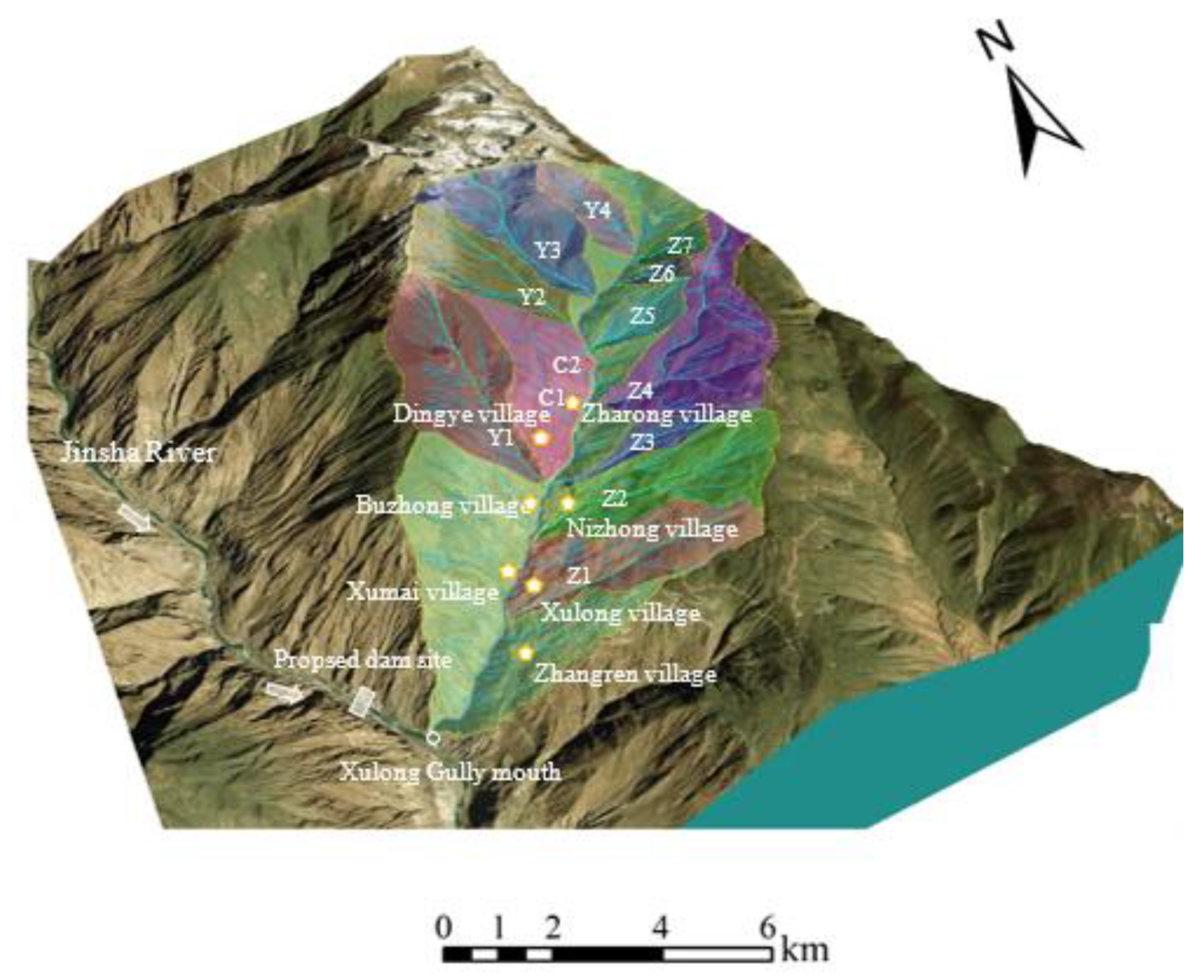
The Xulong Gully drainage basin is located in Derong County of Sichuan Province, China, on the left bank of the upper reaches of the Jinsha River at the border between Sichuan and Yunnan Provinces. The Xulong Gully estuary is only about 2 km away from the proposed dam site for a hydropower station in the upper reaches. Xulong Gully Valley covers an area of 55.62 km
2, the basin mainly receives atmospheric precipitation and ice melt water recharge, and the flow varies with the seasons, with large flow in summer and small flow in winter. The length of the main Xulong debris flow gully is 12.39 km, with 7 branches on the left side of the main trench and 4 branches on the right side.
Table 1 shows the geometric characteristic parameters for the drainage basin of Xulong Gully. The Xulong Gully estuary is located near the dam site, and the activity and scale of debris flow there may affect safe operation of the proposed power station and ancillary facilities (
Figure 1).
The study area is a canyon landform type, the overall topography is high in the northwest and low in the south and east, the climate is a plateau climate zone, the average annual temperature is 14.5 °C, the average annual precipitation is 385 mm, and the average annual evaporation is 2308 mm.
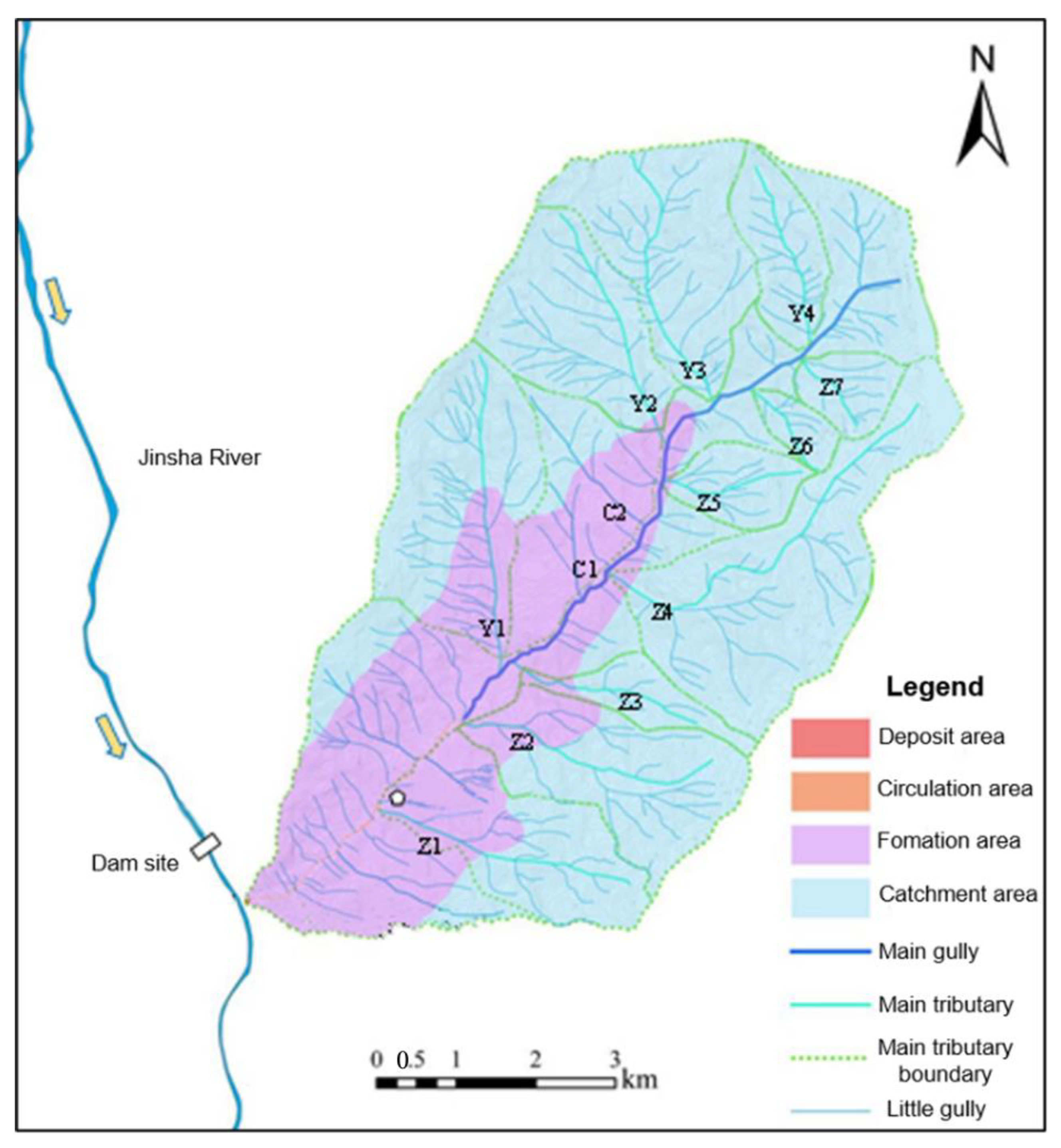
Based on a field investigation and remote sensing interpretation, Xulong Gully can be divided into a clear water area, formation area, circulation area, and accumulation area (
Figure 2). The clear water area is located in the high-altitude area of the basin, where the bottom elevation of the left bank is 3300 m and that of the right bank is 3600 m. This section has strong confluence conditions. Rainfall is collected into slope runoff and groundwater recharge occurs, providing the necessary hydrodynamic conditions for debris flow initiation and material transport. The formation area and circulation area are below the clear water area, with the runoff from the clear water area acting on this section. Once the solid material in and near the gully channel is transported by the runoff, mountain torrents or debris flow will form. During debris flow in this section, the loose solid material in the gully bed is flushed away and the feet of the bank slopes on both sides of the gully channel are eroded laterally, which can cause bank slope instability, providing added provenance for the debris flow. Debris flow migrates through this section to the accumulation area at the Xulong Gully estuary prior to entering the Jinsha River.
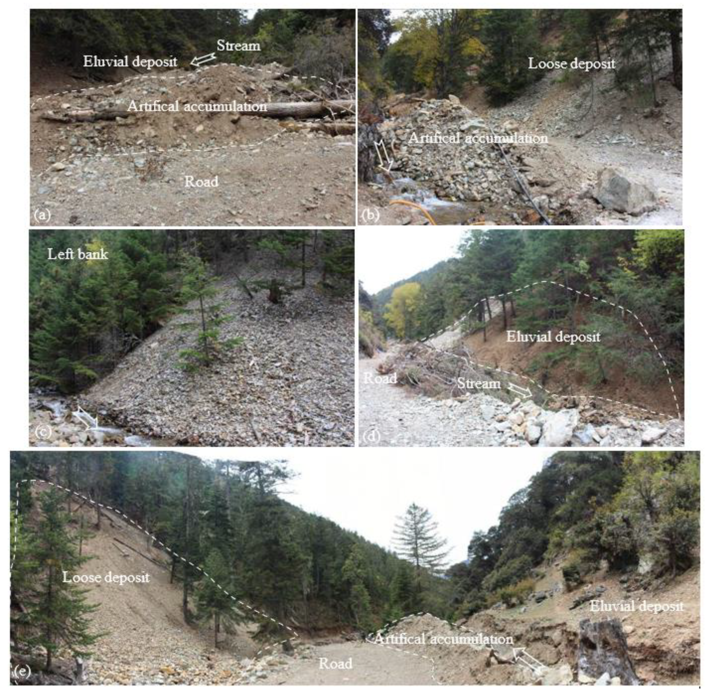
The loose solid material of the debris flow in the Xulong Gully drainage basin originates from five sources: (1) natural collapse of material into the basin caused by physical weathering, particularly under extremely cold conditions, mainly distributed in the strong weathering zone at an altitude over 4200 m, as well as natural collapse of material along the bank slope at and below 2500 m due to the arid climate; (2) loose deposits in the gully channels; (3) collapse and landslides caused by cut slopes on highways, (4) artificial deposits, and (5) provenance provided by early landslide mass in the lower reaches. Typical provenance accumulation is shown in
Figure 3. According to the field investigation, in Xulong Gully, the total volume of provenance that can be supplied for debris flow is about 91.90 × 10
4 m
3.
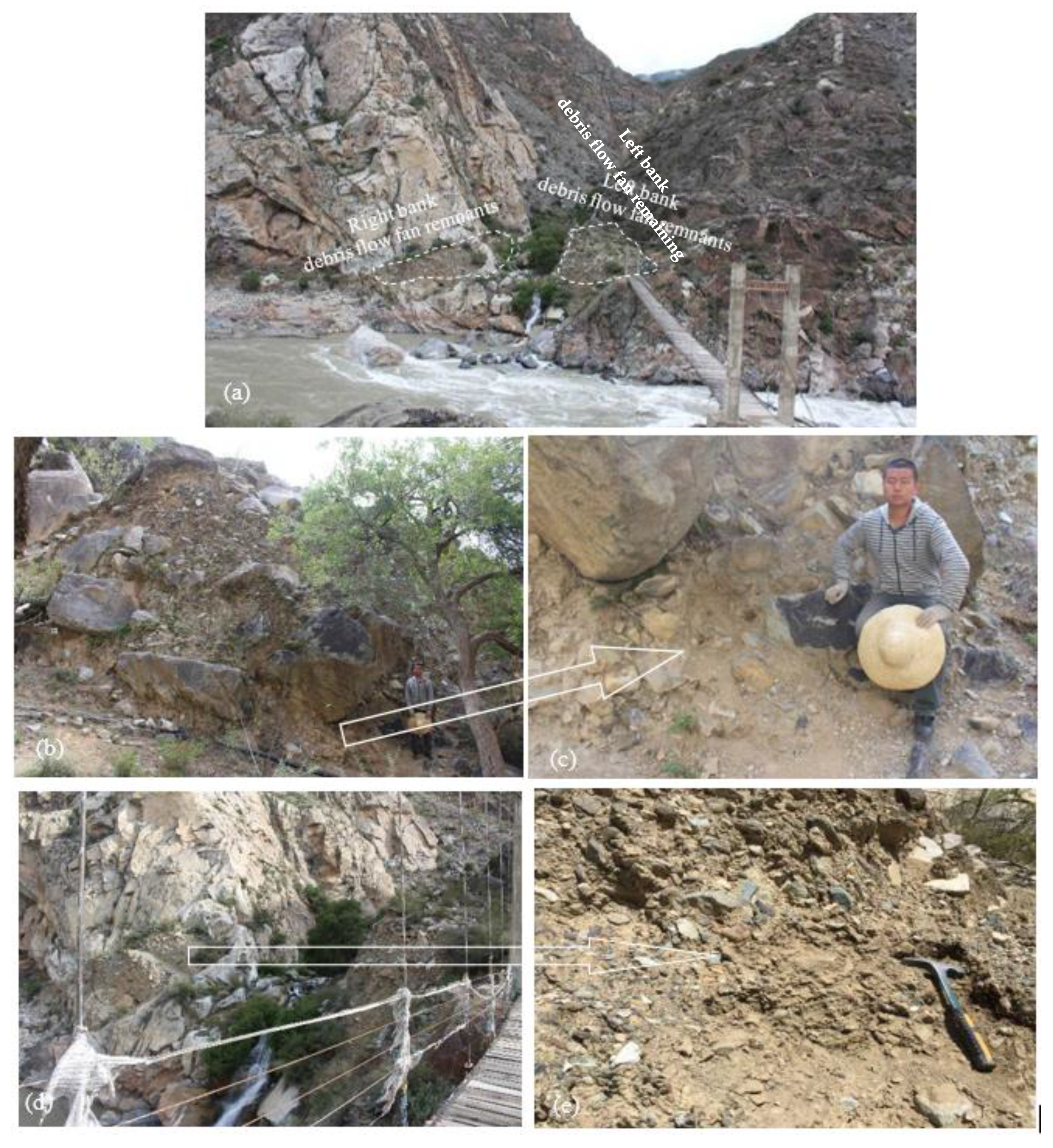
Xulong Gully once saw large-scale debris flows, with a debris flow fan remaining at the Xulong Gully estuary (
Figure 4). Based on the site investigation and environmental conditions for debris flow disasters, along with the
Code for Investigation of Debris Flow Disaster Prevention and Control Engineering (DZ/T0220-2006), the volumetric weight of the debris flow was estimated as 1.6 t/m
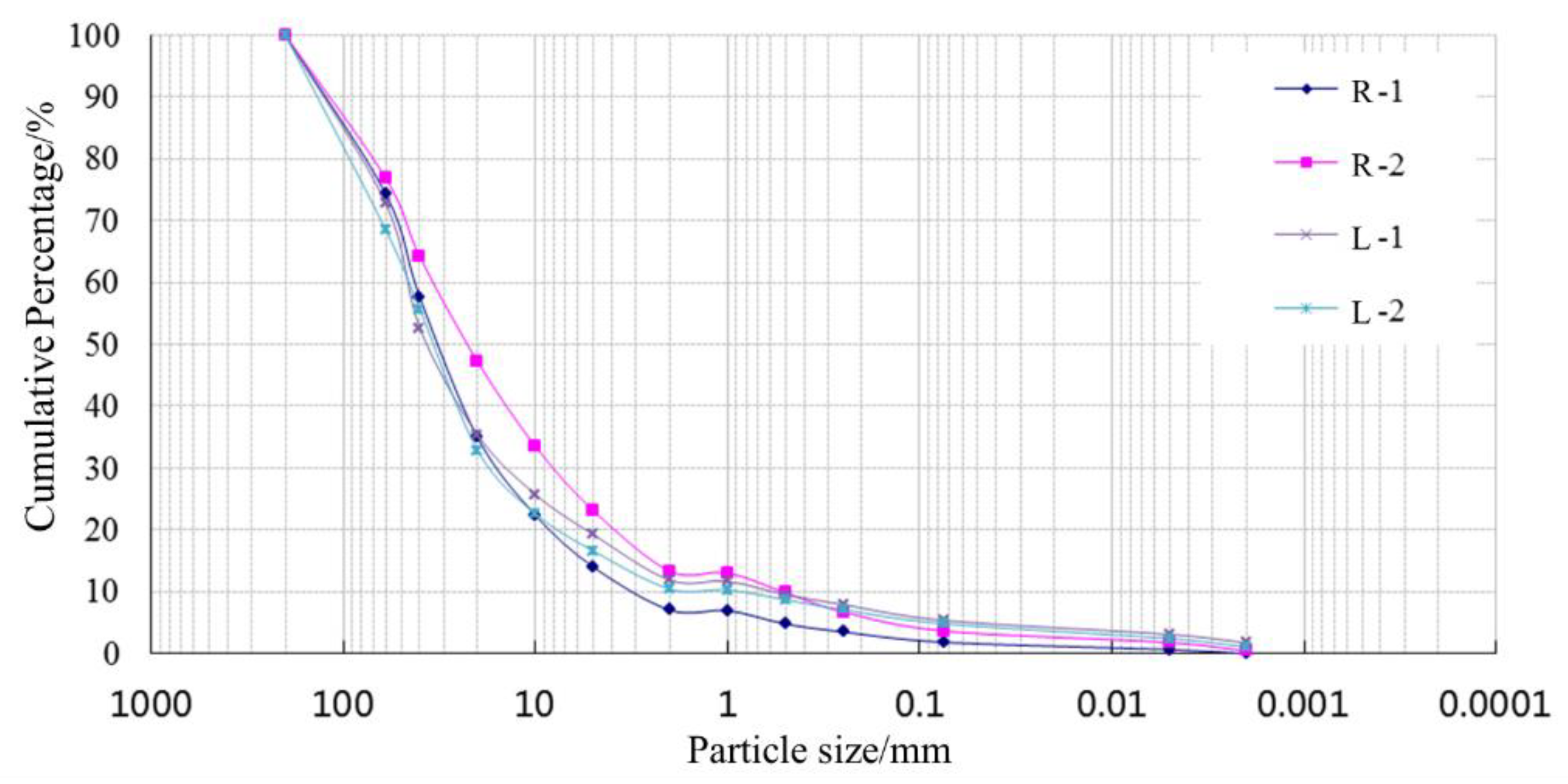
3. To study the grain size composition of early accumulations, samples were collected from the early accumulations on the left and right banks of Xulong Gully for an onsite sieve analysis test. Two sets of parallel samples were taken from each sampling point. Since geosieves have a maximum mesh size of 60 mm, they are not suitable for analysis of gravel larger than 200 mm; the volume of gravel larger than 200 mm was estimated to be 9% using delineating windows onsite. For particle sizes between 1 and 200 mm, field sieve analysis and static water sedimentation tests were carried out, with the size distribution results shown in
Figure 5. In the sieved soil samples from the right bank, the percent particle size < 2 mm was 10.67%, while the percent particle size < 0.5 mm was about 7.3%. In the sieved soil samples from the left bank, the percent particle size < 2 mm was 11.16%, while the percent particle size < 0.5 mm was about 9.1%. In combined sieved soil samples from the left and right banks, the average percent particle size < 2 mm was 10.92%, while the average percent particle size < 0.5 mm was 8.2%. The amount of finer particulate matter in the samples was small (
Figure 5). Therefore, if debris flow is formed, the debris flow fluid property tends to be dilute, and its type tends to be the water-stone type. There are rock blocks with a size of about 3 m in the accumulation fan, indicating that debris flows in this area have strong transport capacity. In addition, the field investigation identified several mud marks in the debris flow circulation area, with the highest mud marks about 1.6 m above the bottom of the gully. This indicates that large-scale debris flows have historically occurred in Xulong Gully, affecting the entire gully estuary.
Thus, if a large-scale debris flow occurs in Xulong Gully, it may pose a substantial threat to the engineering area of the power plants. Therefore, the potential range of debris flows that could occur in Xulong Gully was evaluated.
3. Numerical Calculation Method for Shallow Flow Model
In computational fluid dynamics, a fluid can be considered shallow flow if its planar scale is much larger than its vertical scale. In this study, a two-dimensional shallow water equation was used to simulate debris flow [
22]. Two-dimensional shallow water equations have been widely used to describe fluids with horizontal dimensions much larger than their vertical dimension, such as floods in mountainous areas and river flows. By assuming that the fluid satisfies uniformity of hydrostatic pressure and velocity in the vertical direction, the three-dimensional incompressible Navier-Stokes equation can be simplified to a two-dimensional depth-averaged mass and momentum balance equation, i.e., the two-dimensional shallow water equation, whose vector format is:
where,
and where
h denotes the water depth,
Zb denotes the foundation altitude,
g denotes gravity acceleration, and
qx(
=uh) and
qy(
=vh) denote the discharge per unit width in the
x and
y directions, respectively.
Sfx and
Sfy denote the flow friction resistance coefficients in the
x and
y directions, respectively.
Debris flow fluid is different from ordinary water and its friction behavior has specific characteristics. At present, various debris flow friction models have been proposed, such as the Coulomb friction model, Voellmy friction model, and rheological friction model. Through comprehensive analysis, a rheological friction model was selected, as it incorporates the frictional properties, viscosity properties, and contact energy loss of solid particles of the debris flow fluid. Specifically, a secondary rheological friction model, which takes into account viscous and disordered effects in shallow flows, has been widely used to model the frictional behavior of debris flow fluids [
22]. Its expression is as follows:
where
denotes the bottom bed friction term,
S1 denotes the fluid yield factor,
S2 denotes the fluid viscosity factor,
S3 denotes the fluid disturbance diffusion factor,
τ denotes the yield stress,
ρm denotes the density of the solid material in the debris flow,
K denotes the resistance coefficient,
β denotes the debris flow viscosity,
ntd denotes the equivalent Manning resistance coefficient, and
U denotes the shallow flow velocity.
According to the above equation, the bottom bed friction terms in the
x and
y directions can be deduced, as follows:
Yield stress can be expressed as:
Debris flow dynamic viscosity can be expressed as:
where
α1,
α2,
β1, and
β2 denote empirical coefficients.
Cv is the solid volume concentration in the debris flow and can be expressed as:
where
Vs denotes the solid volume in the debris flow and
Vw is the volume of the water in the debris flow.
In addition to bottom bed friction, there is also a term for the bottom bed slope. After being discretized by the central difference method, it is expressed as follows:
where Δ
L denotes the grid spacing.
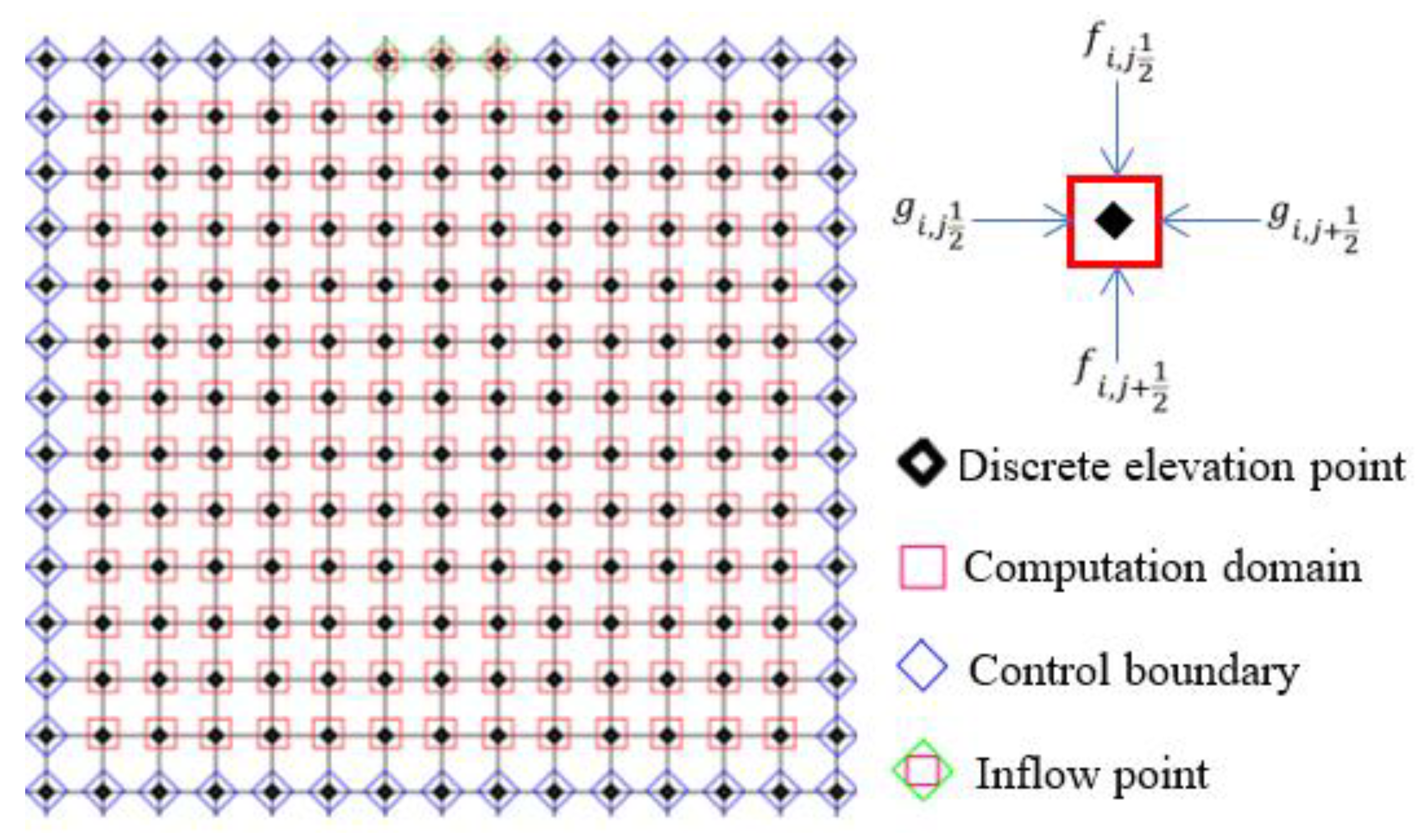
To obtain a realistic complex terrain, gridding was performed using a digital elevation model (
Figure 6). The average elevation value for the grid was used to replace the overall elevation value for the grid, and the elevation value was defined at the center of the cell grid. For the governing equation of shallow flow movement, the conserved variable was defined at the center of the cell grid and the finite volume method was used to discretize it, as follows:
where Δ
t denotes the time step; Δ
x and Δ
y denote the grid size in the
x and
y directions, respectively; and
i and
j represent the unit subscripts.
The time step Δ
t of the numerical calculation can be expressed by the following equations:
where
C is a constant (0 ≤
C ≤ 1). The smaller the value, the more stable the solution, but the calculation time and cost increase. In this study, the value of
C was 0.3.
The linear slope reconstruction technique was used to linearly distribute the data in a single grid. When the water depth in the grid was greater than the threshold, the momentum equation for the governing equation of the corresponding grid was solved. However, when the water depth in the grid was smaller than the threshold, the momentum equation was not solved. In this study, the water depth threshold set for the dry and wet demarcation was 0.001 m. For efficient calculation, in each iteration the grids involved in the calculation included wet grids (with water depth greater than the threshold) and dry grids adjacent to wet grids. The updated water depth was obtained by solving the governing equations continuously until the final step was calculated.
To simulate debris flow using this model, the digital elevation model is first converted into ASCII files, then the debris flow starting position is selected, i.e., the inlet point location. The debris flow starting position in the study area basin was determined based on the field investigation and remote sensing interpretation. In numerical simulation of the debris flow, the calculations are performed along the flow process line of the debris flow. Finally, the simulation results are obtained after inputting the appropriate model parameters.
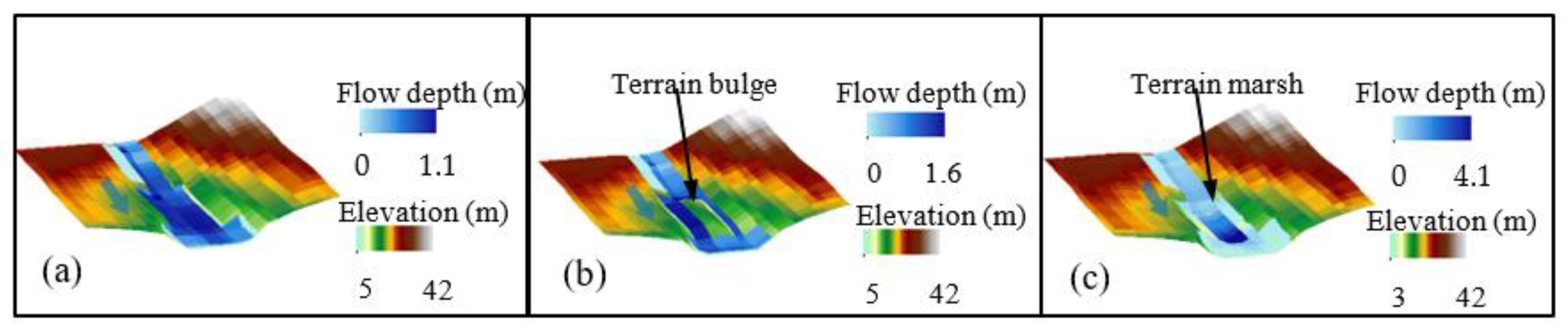
To validate the proposed model, a group of virtual test was conducted to test whether the proposed model can adapt to complex terrain. To conduct the test, three types of irregular terrain were constructed, downhill original terrain, downhill convex terrain, and concave terrain. The undulation of the convex terrain and the concave terrain was 3 m. The raw data accuracy of the digital terrain model was 30 m for the terrain and its plane range was 100 m × 100 m, which was converted into a terrain raster of 5 m × 5 m. In the simulation, the fluid inflow velocity was set to 30 m
3/s and the total simulation time was set to 80 s. The simulation results are shown in
Figure 7. The maximum fluid flow depth in the original terrain was 1.1 m (
Figure 7a). When 3 m raised terrain was placed in the lower reaches, the fluid that originally had a maximum flow depth of 1.1 m could only bypass the raised terrain (
Figure 7b). When 3 m depressed terrain was placed in the lower reaches, the maximum fluid flow depth became 4.1 m, with an increase in the maximum flow depth consistent with the terrain depression. The test demonstrated that the shallow flow model used in this study can adapt to complex terrain and has the ability to numerically simulate the movement characteristics of shallow flows in complex terrain.
4. Simulation and Prediction of Debris Flow Run-Out in Xulong Gully
Based on the sieving data for the accumulated fan materials, the coarse particles in the non-slurry portion of the historical debris flow fluids are composed of large and small rocks, gravel, and coarse sand. The percent clay (<0.005 mm) in the debris flow samples in the accumulation area was 2.65%, and that of medium fine sand, silt, and clay particles (<0.5 mm) was 12.2%. The percentage of fine particulate matter was very low in the samples, particularly for silt and clay. The fluid in the debris flow should be the diluted and, therefore, they should have low viscosity. In this study, the viscosity coefficient for the numerical simulation was set to a relatively low value of 10 pa·s according to previous literature [
28,
29]. Based on field measurements, the solid density in the debris flow set to 2650 kg/m
3. The riverbed in Xulong Gully is composed of pebbles and rock blocks, with large boulders in between. Its bottom is uniform while its bed surface is uneven. The roughness coefficient for the riverbed in the circulation area was set to 0.04 [
29]. Based on the field investigation, the maximum thickness of the historical debris flow fan in the Xulong Gully estuary was 10 m. The viscosity coefficient for the numerical simulation in this study was set at a relatively high value of 10 kPa. In addition, the inter-layer friction coefficient for the fluids was set at an empirical value of 2500. The values of the empirical parameters
α1,
α2,
β1, and
β2 were set to 0.811, 0.00462, 13.72, and 11.24, respectively [
29,
30], based on the material properties of the debris flow. For the hydrograph of the debris flow run-out, a classical isosceles triangle was adopted for this study [
31,
32], with the duration of the debris flow run-out assumed to be 30 min.
Based on the field investigation, the debris flow catchment area in the main trench of Xulong Gully is mainly from the area of early accumulation of Xulong Gully toward the Gully source, so the debris flow should form near this location. This position also serves as the boundary between the formation area and circulation area of the debris flow, and was selected as the debris flow inflow position in this study. The total provenance volume was 91.9 × 10
4 m
3. From a conservative engineering perspective, it was assumed that all of the provenance was flushed out by one debris flow. Based on Equation (8), the total provenance in one debris flow process under this design condition would be 255.7 × 10
4 m
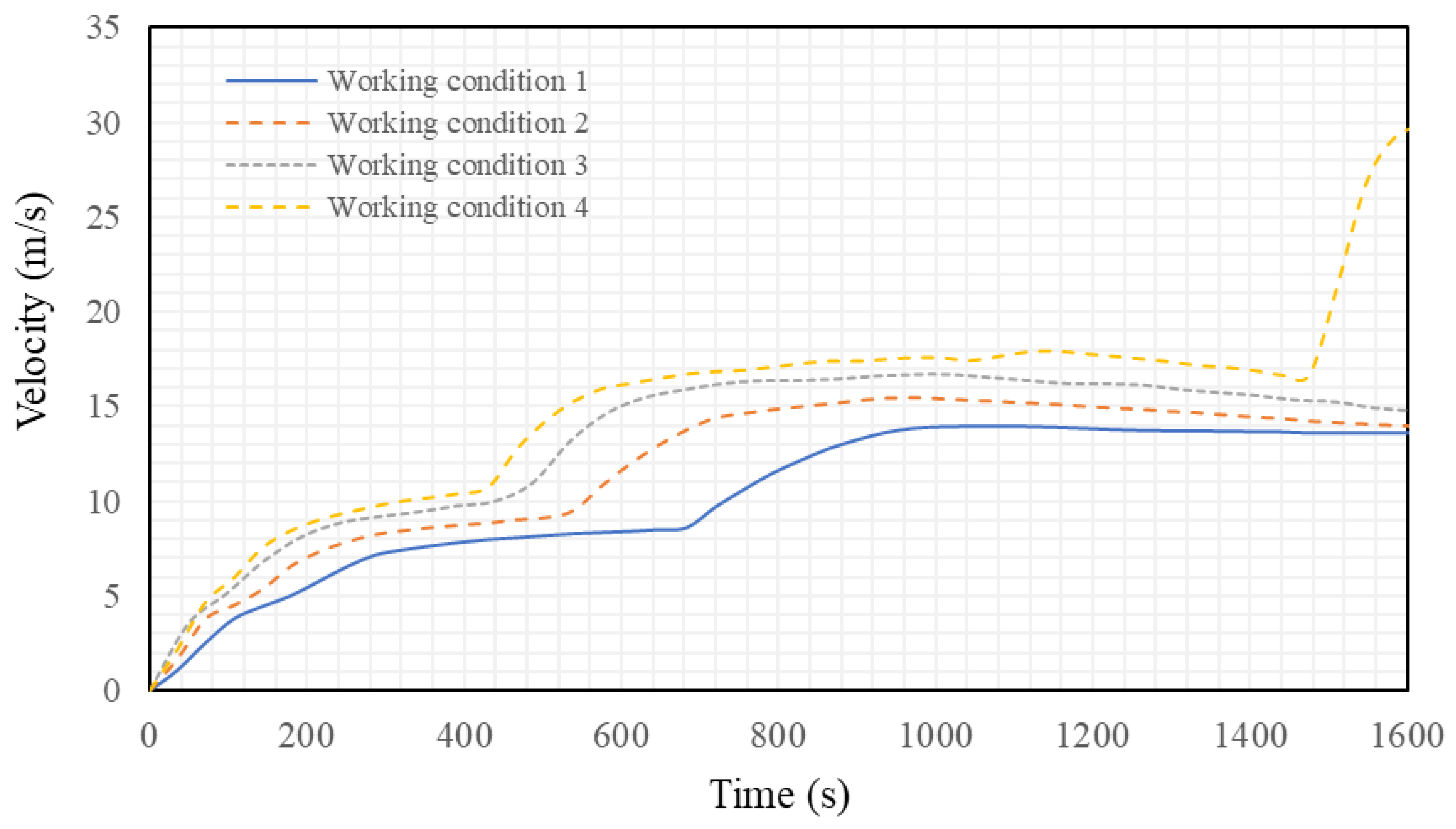
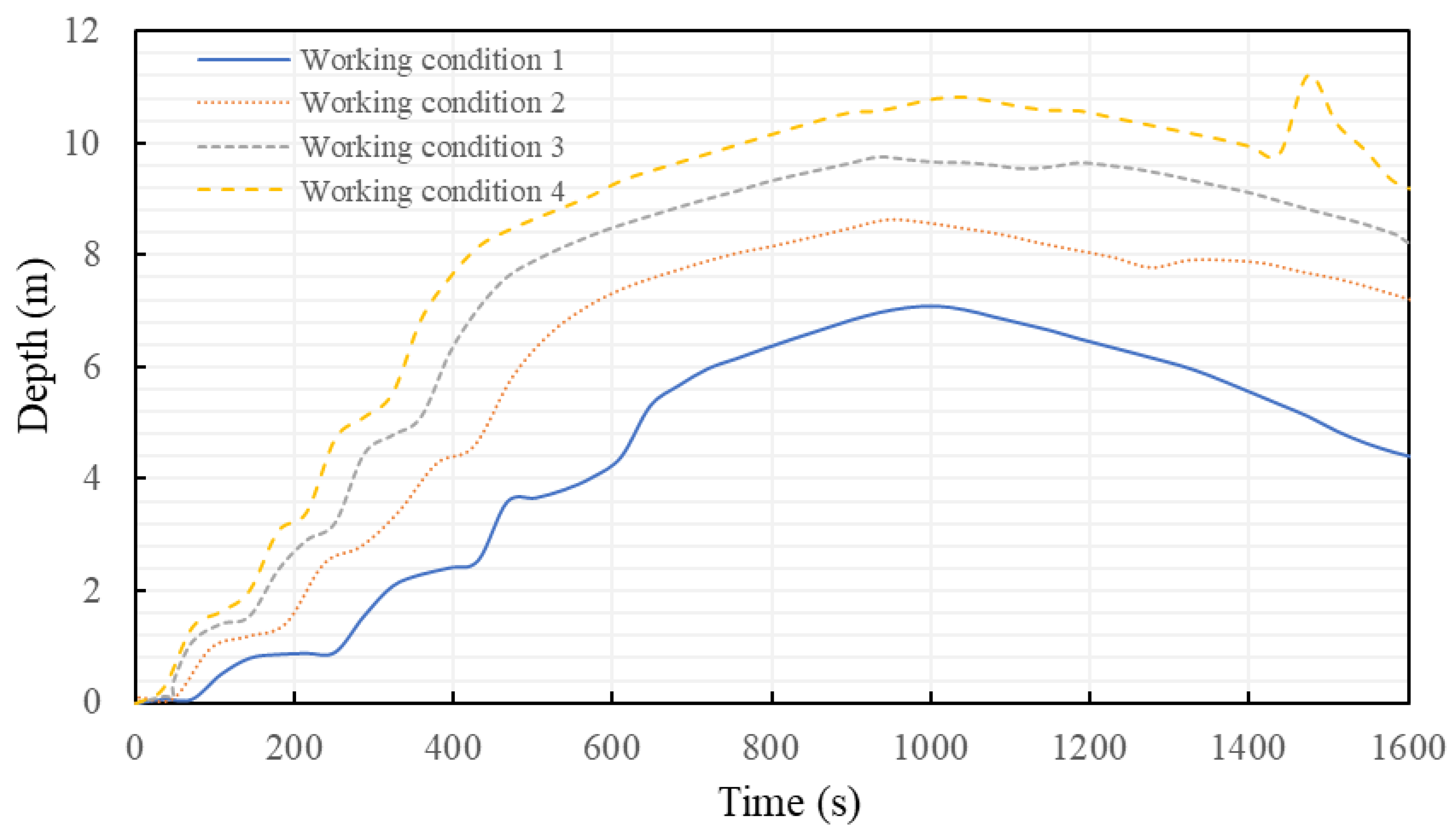
3. However, in actuality, not all of the provenance could be carried and flushed out completely by a single debris flow process. Thus, in this study, a reduction method was used to calculate results for various provenance conditions of 25% (working condition 1), 50% (working condition 2), 75% (working condition 3), and 100% (working condition 4).
Table 2 shows the results for the total amount of debris flow in one process under these four working conditions.
Figure 8 shows the flow velocity of the debris flow under these working conditions and
Figure 9 shows the flow depths process.
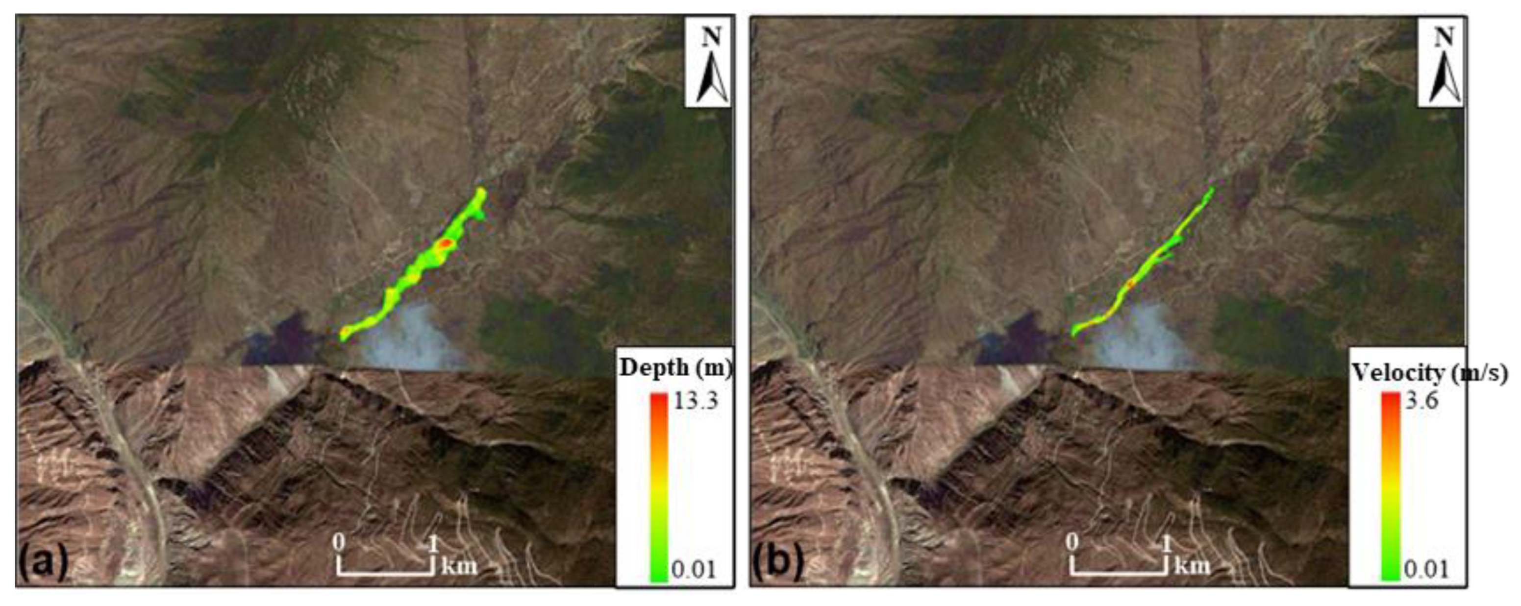
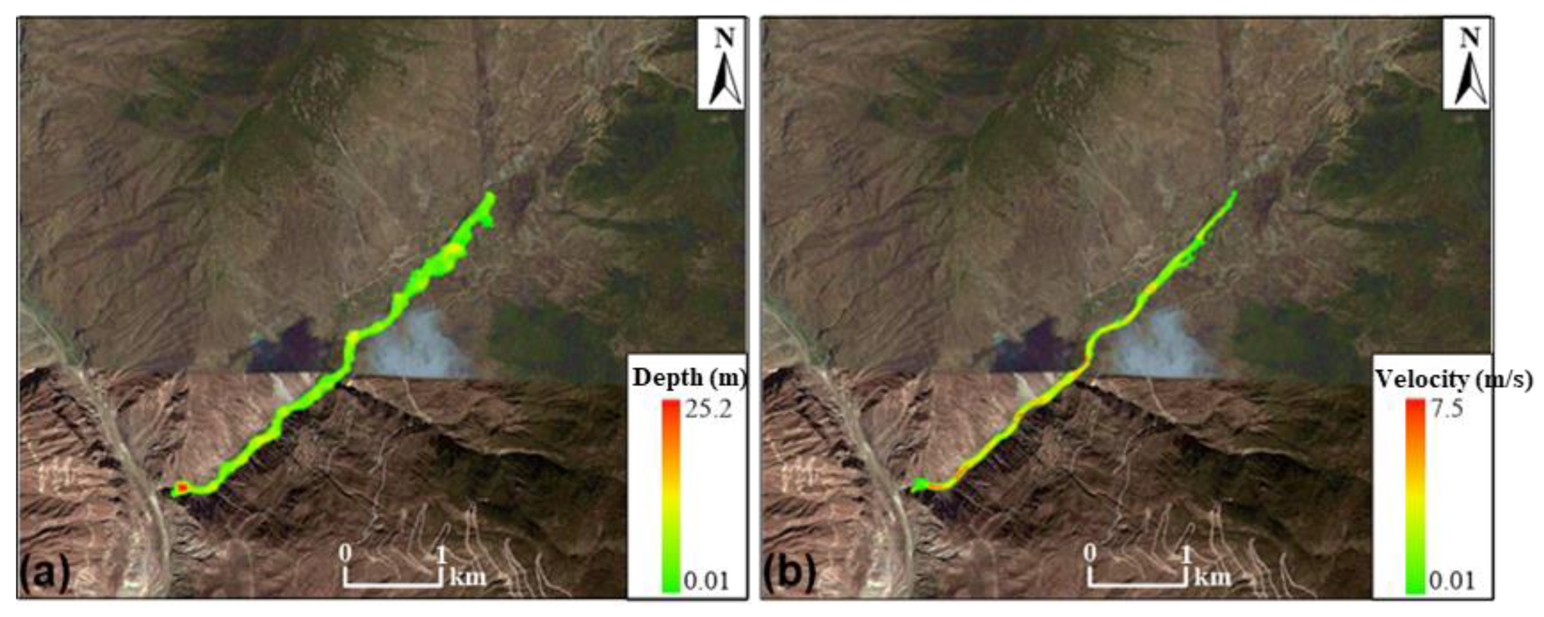
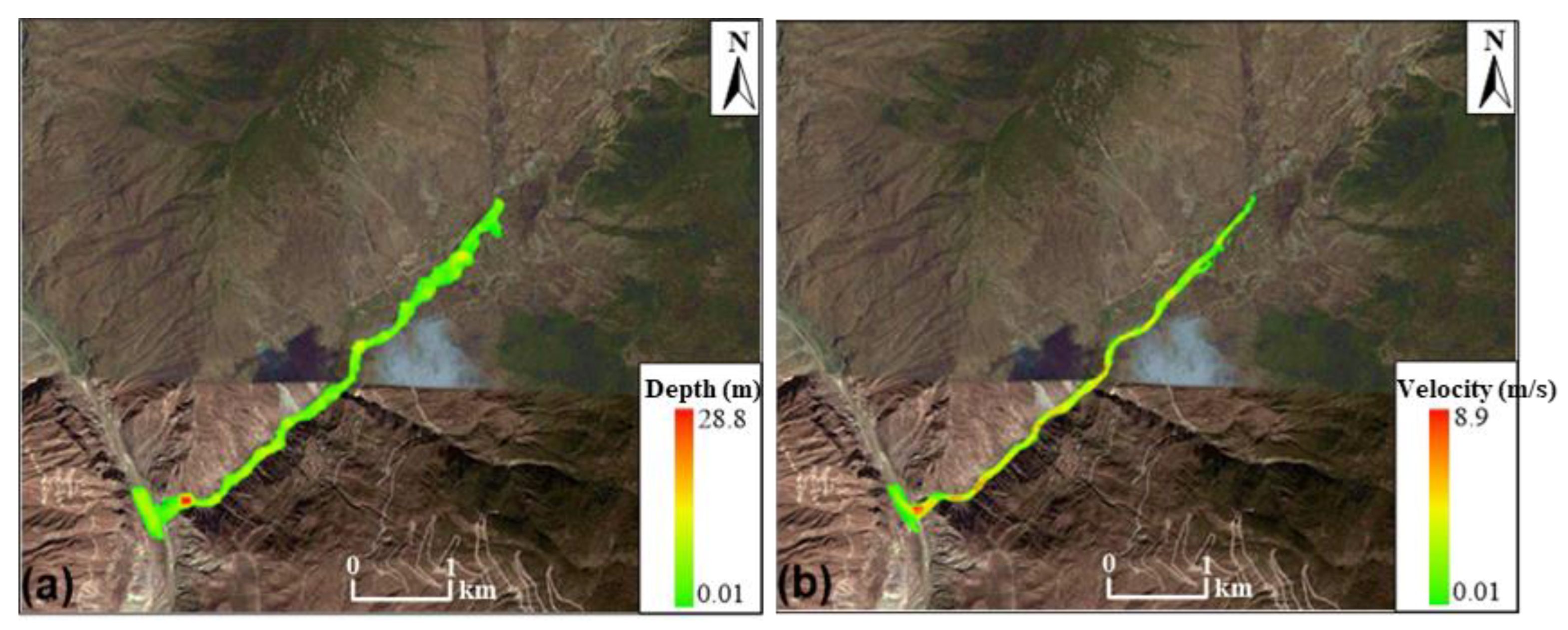
Figure 10,
Figure 11,
Figure 12 and
Figure 13 show the cloud diagrams for the final flow depth and flow velocity at the end of the simulation.
The maximum velocities of the debris flows in the simulations were 6.7–11 m/s (
Figure 10). When the debris flows to the section near the Xulong Gully estuary under working conditions 3 and 4, a waterfall develops in this section, the terrain drops sharply, and the flow depth and flow velocity increase sharply (
Figure 11,
Figure 12 and
Figure 13); the cloud diagrams for flow velocity and flow depth best depict the situation in this area (
Figure 14). The maximum debris flow thickness reached 25.2–28.8 m. Thus, the solid accumulation thickness in this area was 8.9–10.2 m, consistent with the results of the field investigation. In summary, as shown in the cloud diagrams for flow depth and velocity under the four working conditions, when the total debris flow amount in one process is <2 million m
3, the debris flow impact range remains within in Xulong Gully. When the total debris flow amount in one process in the Xulong area > 2 million m
3, the debris flow material will be flushed out into the Jinsha River, blocking a portion of the river.
The total debris flow volume selected for the numerical simulation is used throughout the calculations from debris flow formation to debris flow run-out, including the flow and accumulation processes of the debris flow. The velocity of the debris flow and the flood area size are related to the total debris flow volume in one process, and this volume in turn strongly affects the velocity of the debris flow and the flood area size. Based on the simulation results, the maximum velocity of the debris flow calculated for working condition 4 was 11 m/s and the solid thickness in the debris flow at the Xulong Gully estuary was 8.9–10.2 m. The velocity of debris flow and the solids accumulation thickness in the debris flow at the Xulong Gully estuary is consistent with the scale of historical debris flows. Using the standard section method, the velocity of historical debris flows was calculated as 8.76 m/s and the thickness of the debris flow accumulation fan at the Xulong Gully estuary was measured as 10 m. Thus, numerical simulation can directly and explicitly reflect the entire process of flow and accumulation of the debris flow, which has great value for evaluating the potential impacts of debris flows in the basin.
It is worth noting that if all the solid provenance in the Xulong Gully were flushed out, the Jinsha River would eventually be blocked and a landslide dam about 470 m long would be formed. This would inevitably have a major impact on the dam site of the power stations. Therefore, measures should be taken to modify the debris flow gully, reduce the provenance volume, or block or discharge the potential debris flow, to reduce the potential damage of debris flows and avoid impacting the hydropower stations.
5. Discussion
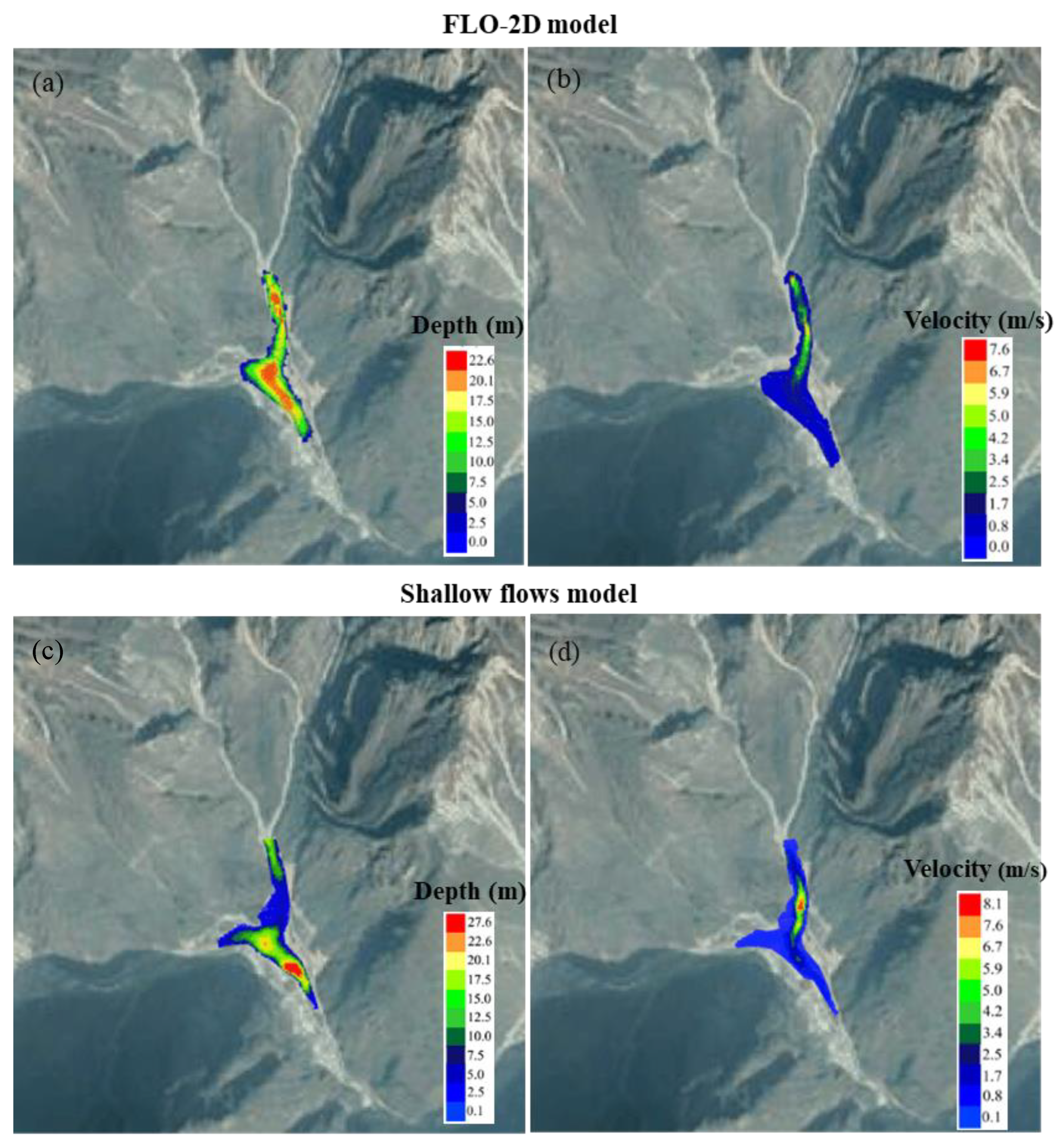
The shallow-water flow model has been widely applied for debris flow simulation, and the Flo-2D model is one of the most common. The Flo-2D model is a kind of shallow-water flow model based on the finite difference method. In this section, we compared our model with the Flo-2D model. We selected a case study of Xiaojiagou from the literature [
28] for verification through a way of comparing the debris flow deposit area. The basic parameters and settings for the model were described in the literature, with the simulation results shown in
Figure 7. The results of the comparison showed that the maximum flow depth of the debris flow calculated by Flo-2D was about 22.6 m, and that calculated by the shallow flow model in this study was 27.6 m. The maximum flow velocity of the debris flow calculated by Flo-2D was about 7.6 m/s, while that calculated by the shallow flow model in this study was 8.1 m/s. The overall results were similar. From the perspective of debris flow morphology, the simulation results of the shallow flow model used in this study were also very similar to those from the Flo-2D model on the whole. Considering that there may have been some differences in the topographic data, time step settings, etc. used in the simulation that may lead to differences in the simulation results, the small differences between the results of the two models were considered acceptable. Thus, the shallow flow model presented in this study can solve the problem of debris flow simulation.
Although simulation results between our model and the Flo-2D model are generally very similar, there are still some differences between them because of different basic numerical frames. By simulating the same debris case in Xiaojia gully based on our model and Flo-2D model, some caparisons were carried out to reflect the characteristics of our model: (1) our numerical model can guarantee the conservation characteristics of water quantity and momentum theoretically; (2) Flo-2D model based on finite difference method needs to search for all meshes in the computational domain while our model only searches for the wet meshes and adjacent dry meshes, improving computational efficiency [
22,
33]; (3) our model can simulate a flow over highly irregular topography precisely and stably; (4) a limitation of our model is that only one inflow point can be set during the simulation. This means that our model can only temporarily simulate the dynamic process of a single debris flow. It is difficult to simulate the dynamic processes of several debris flows in a small catchment. Developing a multi-inflow points model is our future work.
In general, with the recent rapid development of computational methods, numerical simulation has become a viable tool in the run-out analysis of debris flows. However, one challenge in applying them is to develop robust numerical schemes that can well simulate them over highly irregular topography with complex geometry [
34,
35,
36]. In this study, we bring a well-balanced numerical scheme that adopts effective techniques, such as the linear reconstruction method and the fully implicit scheme to ensure the accuracy and stability of the numerical scheme over irregular topography. In addition, to enhance and strengthen the application ability of the present numerical scheme in debris flow numerical calculation, further work in the future should consider some additional factors, such as the channel erosion, initial conditions of the debris flow, and the rheological properties of the debris flow materials.


