Intelligent Inversion Analysis of Hydraulic Engineering Geological Permeability Coefficient Based on an RF–HHO Model

Abstract

The permeability of the natural geology plays a crucial role in accurately analyzing seepage behavior in the project area. This study presents a novel approach for the inverse analysis of the permeability coefficient. The finite element model (FEM) combined with orthogonal experimental design is used to construct a sample set of permeability coefficient inversion. The established random forest (RF) algorithm surrogate model is applied to determine the optimal values of permeability parameters in the project area using the Harris hawk optimization (HHO) algorithm. This method was used to explore and verify the distribution of natural seepage fields for the P hydropower station. The results showed that the RF model outperformed the classical CART and BP models at each borehole regarding performance evaluation indices. Furthermore, the water head prediction results were more accurate, and the RF model performed admirably in terms of prediction, anti-interference, and generalization. The HHO algorithm effectively searched for the optimal permeability coefficient of the geology. The maximum value of the relative error of the borehole water head inverted was 1.11%, and the accuracy met engineering standards. The initial seepage field distribution pattern calculated followed the basic distribution pattern of the mountain seepage field.

1. Introduction

In recent years, China has built a considerable number of new high dams and large reservoirs, pumped storage power plants, water transfer projects, and other large-scale water conservancy projects, encouraging the sustainable and healthy growth of the economy and society. To ensure the safe construction and normal operation of the project, it is vitally necessary to master the seepage distribution in the project area. As a result, numerical simulation methods are commonly employed to judge the seepage properties. However, this procedure is based on the determination of the permeability coefficient of the natural stratum [1]. The inversion analysis based on onsite observation data can more accurately obtain permeability parameters than indoor and in situ experiments [2], making it one of the most effective ways to determine the permeability coefficients of materials [3]. Many inversion methods [4,5,6,7] have been proposed. However, these classic methods necessitate many calls to the seepage analysis forward model, which is computationally time-consuming and inefficient. Therefore, practical approaches must be adopted to improve the calculation efficiency of inversion methods.

As a method to improve the efficiency of the inversion, surrogate models based on machine learning algorithms have been widely used in recent years. The response surface technique [8], radial basis function (RBF) [9], extreme learning machine (ELM) [10], backpropagation (BP) neural network [11], support vector regression (SVR) [12], multiple adaptive regression splines (MARS) [13], and others are commonly used as surrogate models. These models generate learning samples using FEM. Then, the mathematical model is used to build the relationship between the permeability coefficient (i.e., input variable) and the water head (i.e., output variable). This can then be used to replace the seepage forward model to solve the problem quickly.

Applying the surrogate model can enhance the computational efficiency of the inversion, but its essence remains the standard inversion method of “forward problem inverse calculation”. The parameters inverted are not optimal and have low accuracy; hence, further research into novel seepage inversion theories and methods is required. Chi et al. [9] studied the inversion of permeability coefficients of the high-core rockfill dam using the RBF model and the particle swarm optimization (PSO) algorithm. Ni et al. [14] established a surrogate model based on SVR. They searched for the optimal permeability coefficients of the partition inverted for the Nuozhadu high-core rockfill dam using the PSO algorithm. Li et al. [15] established an inversion analysis model based on the relevance vector machine model and cuckoo search algorithm. They determined the permeability coefficient of each stratum in the study area. Shu et al. [16] used ELM and an optimization algorithm to perform a back study on the permeability coefficient of the dam anti-seepage curtain and determined its optimal value. These studies showed that it is feasible to invert the optimal values of seepage parameters using an optimization algorithm combined with the surrogate model, whereby the inversion accuracy is improved.

In the process of nonlinear modeling of the permeability coefficient, the above model exhibits several problems, including low prediction accuracy, poor robustness, slow convergence speed, limited generalization ability, and quickly falling into a local minimum. Additionally, the model assumes the medium to be isotropic during inversion, disregarding the impact of its anisotropy on seepage behavior. Given this, this study introduces the random forest (RF) algorithm, considers the anisotropic characteristics of the medium, and constructs a surrogate model for seepage analysis. Then, Harris hawk optimization (HHO) is introduced to establish a new inversion model that can intelligently optimize the stratum permeability coefficient and lay the foundation for safety analysis of seepage properties in the project area. Lastly, the rationality and validity of the model proposed are verified using an engineering example.

2. Methodology

2.1. Random Forest (RF)

RF [17] is an ensemble learning algorithm widely used for nonlinear regression problems [18,19]. The algorithm’s core is to use the ensemble learning method (i.e., bootstrap aggregating) to model the decision tree for each sample set extracted using the bootstrap method. A single decision tree with overfitting and local convergence problems becomes multiple “forests”, improving the model’s performance. The implementation steps are as follows:

Step 1: T training sets S₁, S₂, …, S_T are randomly generated using the bootstrap method. Let the set of samples be $S=\left\{x_1,x_2,\cdots ,x_n\right\}$; there is putback from the set of samples S to draw n times, forming a new set of samples S_i (i = 1, 2, …, T). The total samples of S_i are the same, but it contains only about 62.3% of samples in the original set.

Step 2: According to each training set S_i (i = 1, 2, …, T), the corresponding decision tree models C₁, C₂, …, C_T are generated.

Step 3: The corresponding result C₁ (X), C₂ (X), …, C_T (X) is obtained for the test set of samples X using each of the generated decision tree models.

Step 4: The output results of T decision trees are averaged as the result of the X calculation.

The RF model contains three critical parameters: the number of decision trees N_tree, the number of random characteristics of node splitting M_try, and the minimum number of samples of leaf nodes Node_size. Generally, compared with N_tree and M_try, Node_size has less impact on the performance and efficiency of the RF model, and the default value is generally chosen.

2.2. Harris Hawk Optimization (HHO)

The HHO algorithm is a novel global search algorithm constructed by Heidari et al. [20] on the basis of the predation patterns of the Harris hawk group and Levy flight characteristics. This algorithm has the characteristics of few adjustment parameters, an optimal random search path, easy implementation, and high calculation accuracy [21]. It has been widely applied to mechanical multi-objective optimization [22], dam deformation prediction [23], environmental drought index prediction [24], landslide prediction [25,26], and other fields. This paper introduces the HHO algorithm to search for the optimal permeability coefficient value. The optimization process consists of the exploration phase, the transition from exploration to exploitation, and the exploitation phase. The specific process is described below.

(1)

Exploration phase

In this phase, HHO simulates the Harris hawks’ behavior of tracking prey. Their positions are updated according to Equation (1).

$$X(t+1)=\left\{\begin{array}{l}{X}_{rand}(t)-r_1\left|X_{rand}(t)-2r_{2}X(t)\right|\hspace{0.17em}\hspace{0.17em}\hspace{0.17em}\hspace{0.17em}\hspace{0.17em}\hspace{0.17em}\hspace{0.17em}\hspace{0.17em}\hspace{0.17em}\hspace{0.17em}\hspace{0.17em}\hspace{0.17em}\hspace{0.17em}\hspace{0.17em}\hspace{0.17em}\hspace{0.17em}q\ge 0.5\\ (X_{rabbit}(t)-X_m(t))-r_3(\mathrm{LB}+r_4(\mathrm{UB}-\mathrm{LB}))\hspace{0.17em}q<0.5\end{array}\right.,$$

(1)

where X (t) and X (t + 1) are the positions of hawks in the t-th iteration and t + 1-th iteration, X_rand (t) is a randomly selected Harris hawk individual, X_rabbit (t) is the current location of the prey, and r₁, r₂, r₃, r₄, and q are random numbers in the range [0, 1]. UB and LB are the upper and lower bounds of the search space. X_m (t) is the average position of hawks and is computed as shown in Equation (2).

$$X_m(t)=\frac{1}{N}({\displaystyle \sum _{i=1}^N{X}_i(t)}),$$

(2)

where N is the number of Harris hawks, and X_i (t) is the location of each hawk in the t-th iteration.

(2)

Transition from exploration to exploitation

HHO conducts the transition from exploration to exploitation according to the escape energy of the prey. It is defined as shown in Equation (3).

$$E=2E_0(1-\frac{t}{T}),$$

(3)

where E is the escape energy of the prey, E₀ is a random initial energy between (−1, 1), t is the number of iterations, and T is the maximum number of iterations.

When |E| ≥ 1, the hawks track the prey in different regions, and HHO executes the exploration phase; when |E| < 1, HHO executes the exploitation phase in the neighborhood of the solution, and hawks encircle, approach, and attack the prey.

(3)

Exploitation phase

In this phase, when |E| ≥ 0.5, the hawks conduct a soft besiege on the prey; when |E| < 0.5, the hawks conduct a hard besiege on the prey. In addition, the chance of the prey escaping is measured using r. When r ≥ 0.5, the prey has enough energy to escape; when r < 0.5, the prey does not have enough energy to escape. Therefore, the hawks have the following four strategies to catch the prey.

When r ≥ 0.5 and |E| ≥ 0.5, the hawks execute the soft besiege strategy and update their positions according to Equation (4).

$$X(t+1)=X_{rabbit}(t)-X(t)-E\left|J{X}_{rabbit}(t)-X(t)\right|,$$

(4)

where $J$ is the random jumping strength of the prey in the process of escape, when $J=2(1-r_5)$, and $r_5$ is a random number in the range (0,1).

When r ≥ 0.5 and |E| < 0.5, the hawks execute the hard besiege strategy, and their positions are updated as represented by Equation (5).

$$X(t+1)=X_{rabbit}(t)-E\left|X_{rabbit}(t)-X(t)\right|.$$

(5)

When |E| ≥ 0.5 and r < 0.5, the hawks execute the soft besiege strategy of progressive rapid dives and update their positions using Equation (6).

$$X(t+1)=\left\{\begin{array}{l}Y,f(Y)<f(X(t))\\ Z,f(Z)<f(X(t))\end{array}\right.,$$

(6)

where f is the fitness function. Y and Z are obtained using Equations (7) and (8).

$$Y(t)=X_{rabbit}(t)-E\left|J\cdot X_{rabbit}(t)-X(t)\right|,$$

(7)

$$Z=Y+S\times LF(D),$$

(8)

where D is the problem dimension, S is a D-dimension random variable, with its elements being random numbers in the range [0, 1], and LF is the Levy flight function [19].

When |E| < 0.5 and r < 0.5, the hawks execute the hard besiege strategy of progressive rapid dives, and their positions are updated as described in Equations (9) and (10).

$$X(t+1)=\left\{\begin{array}{l}Y,f(Y)<f(X(t))\\ Z,f(Z)<f(X(t))\end{array}\right.,$$

(9)

where Y and Z are calculated using Equations (10) and (8).

$$Y(t)=X_{rabbit}(t)-E\left|J\cdot X_{rabbit}(t)-\frac{1}{N}({\displaystyle \sum _{i=1}^N{X}_i(t)})\right|.$$

(10)

2.3. Calculation Principle of the Three-Dimensional Stable Seepage Field

According to the continuity equation of water flow, the primary differential Equation [3] of steady seepage is expressed as shown in Equation (11).

$$\frac{\partial }{\partial x}\left(k_x\frac{\partial H}{\partial x}\right)+\frac{\partial }{\partial y}\left(k_y\frac{\partial H}{\partial y}\right)+\frac{\partial }{\partial z}\left(k_z\frac{\partial H}{\partial z}\right)=0,$$

(11)

where H is the water head function, and k_x, k_y, and k_z are the permeability coefficients in x-, y-, and z-directions, respectively.

According to the common boundary conditions [3] and the variational principle, Equation (11) can be solved using Equation (12).

$$I(H)={\displaystyle {\iiint }_{\mathsf{\Omega }}\frac{1}{2}}\left[k_x{\left(\frac{\partial H}{\partial x}\right)}^2+k_y{\left(\frac{\partial H}{\partial y}\right)}^2+\left.k_z{\left(\frac{\partial H}{\partial z}\right)}^2\right]\mathrm{d}x\mathrm{d}y\mathrm{d}z-{\displaystyle {\iint }_{S_2}q}H\mathrm{d}s\Rightarrow \min \right.,$$

(12)

where Ω is the calculation area.

By discretizing the seepage calculation area, the basic finite element equation for solving a three-dimensional seepage field can be obtained [27] from Equation (12) as shown in Equation (13).

$$\left[K\right]\cdot \left\{H\right\}=\left\{F\right\},$$

(13)

where $\left[K\right]$ is the overall penetration matrix, $\left\{H\right\}$ is node head array, and $\left\{F\right\}$ is the corresponding flow matrix.

2.4. The Fitness Function of the RF–HHO Model

The essential purpose of seepage field inversion is to find the optimal combination of permeability coefficients within a given range. Therefore, the essence of the permeability coefficient inversion is an optimization problem. This study used HHO to find the optimal permeability coefficient for the geology, and an inversion model based on RF–HHO was established. The model’s fitness function was the minimum mean square error (MSE) between the measured and calculated water head of boreholes, as shown in Equation (14). The pseudo-code of the RF–HHO model is shown in Algorithm 1.

$$f=\min \mathrm{MSE}=\min \left[\frac{1}{q}{\displaystyle \sum _{k=1}^q{(H_k-H_k^{\prime })}^2}\right],$$

(14)

where $H_k$ is the measured water head value of the k-th borehole, $H_k^{\prime }$ is the calculated water head of the k-th borehole, and q is the number of boreholes.

The constraints of the objective function are shown in Equation (15).

$$\mathrm{s}.\mathrm{t}. x_m^d\le x_m\le x_m^u (m = 1, 2, \dots , M),$$

(15)

where $x_m$ is the permeability coefficient inverted, $x_m^u$ and $x_m^d$ are its upper and lower limits, respectively, and M is the total number of permeability coefficients inverted.

Algorithm 1: Pseudo-code for RF–HHO implementation.

Input: training examples and range of permeability coefficient values Output: Optimal combination of permeability coefficients for the geology of the project area

Initialize N and T, generate the initial population $X_{N\times D}$, and calculate the fitness value f;

While t < T

Set Xrabbit as the prey (best location), and update E0, E, and r for each hawk (Xi)

If |E| ≥ 1 Use Equation (1) to update the population;     if |E| < 1

if r ≥ 0.5 and |E| ≥ 0.5    Use Equation (4) to update the population;

if r ≥ 0.5 and |E| < 0.5    Use Equation (5) to update the population;

if r < 0.5 and |E| ≥ 0.5    Use Equation (6) to update the population;

if r < 0.5 and |E| < 0.5    Use Equation (9) to update the population; end  end

Calculate the fitness value of the new individual, and update their positions and optimal fitness value;

t = t + 1;

end

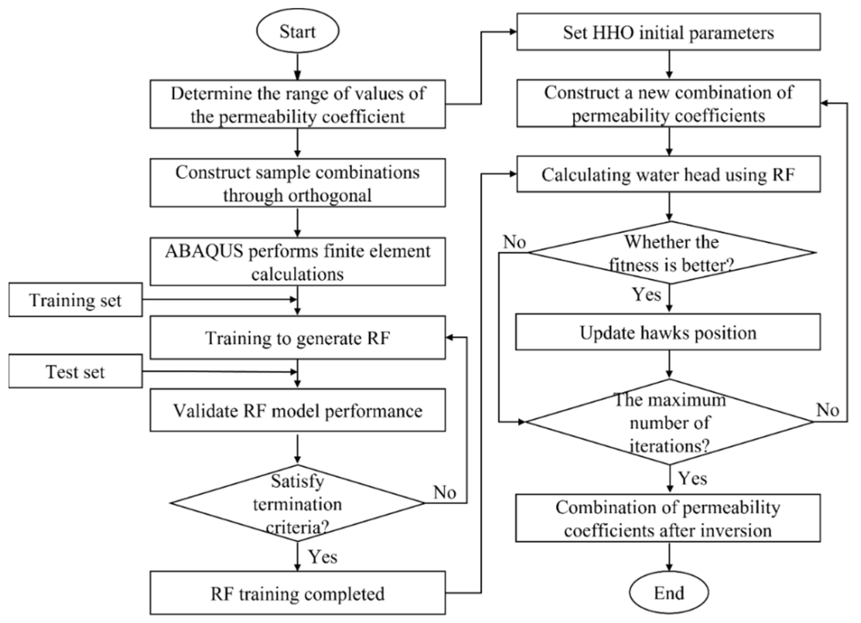
2.5. Establishment of a Permeability Coefficient Inversion Model for the Dam Site Area

Using the RF and HHO algorithms, this paper established an inverse model of geology permeability coefficients. It can intelligently search for the optimal permeability coefficients of the dam foundation. Figure 1 shows the modeling procedure. The main steps are as follows:

Step 1: The orthogonal test design method is used to construct the combination of permeability coefficients. Then, the borehole water head under the corresponding combination is obtained by FEM. Finally, the inversion sample set is established.

Step 2: The permeability coefficient is selected as the input variable of the RF model, and the corresponding borehole head calculation value is selected as the output variable of the model.

Step 3: The sample set is split into 80% for training and 20% for testing. Simultaneously, to eliminate the impact of variable magnitude on the RF model, the sample data are preprocessed using the normalization Equation (16) to limit the data to [0, 1].

$$x_m^{\prime }=\frac{x_m-x_m^d}{x_m^u-x_m^d},$$

(16)

where $x_m^{\prime }$ is the normalized permeability coefficient value.

Step 4: Tenfold cross-validation is used to determine the optimal parameters M_try and N_tree of the RF model. Then, the inversion surrogate model is trained.

Step 5: It is verified whether the accuracy of the surrogate model obtained in Step 4 meets the error threshold. If it meets the standards, the procedure proceeds to the next step. Otherwise, steps 4 and 5 are repeated.

Step 6: After denormalizing the output results, the surrogate model established is evaluated using the following statistical indices [18,19,28,29,30]: mean absolute error (MAE), mean absolute percentage error (MAPE), root-mean-square error (RMSE), and goodness of fit (R²). The calculated expressions are shown in Equations (17)–(20), respectively.

$$\mathrm{MAE}=\frac{1}{n}{\displaystyle \sum _{i=1}^n\left|y_i-{\widehat{y}}_i\right|},$$

(17)

$$\mathrm{MAPE}=\frac{100}{n}{\displaystyle \sum _{i=1}^n\left|\frac{y_i-{\widehat{y}}_i}{y_i}\right|},$$

(18)

$$\mathrm{RMSE}=\sqrt{\frac{1}{n}{\displaystyle \sum _{i=1}^n{(y_i-{\widehat{y}}_i)}^2}},$$

(19)

$$R^2=1-\frac{{\displaystyle \sum _{i=1}^n{(y_i-{\widehat{y}}_i)}^2}}{{\displaystyle \sum _{i=1}^n{(y_i-\overline{y})}^2}},$$

(20)

where $y_i$ and ${\widehat{y}}_i$ are the measured and predicted values, respectively, $\overline{y}$ and ${\overline{\widehat{y}}}_i$ are the averages of the measured and predicted values, respectively, and n is the number of measured values.

Step 7: When employing HHO to find the optimal permeability coefficients, a new combination of permeability coefficients is constructed. Their corresponding borehole head is calculated using the established RF model. If the fitness under this combination is less than the existing optimal fitness, the existing combination and fitness are update. Otherwise, the procedure proceeds to step 8.

Step 8: If HHO does not reach the maximum number of iterations, step 7 is repeated. Otherwise, the current combination and its fitness are updated, along with the final inversion result.

3. Case Study

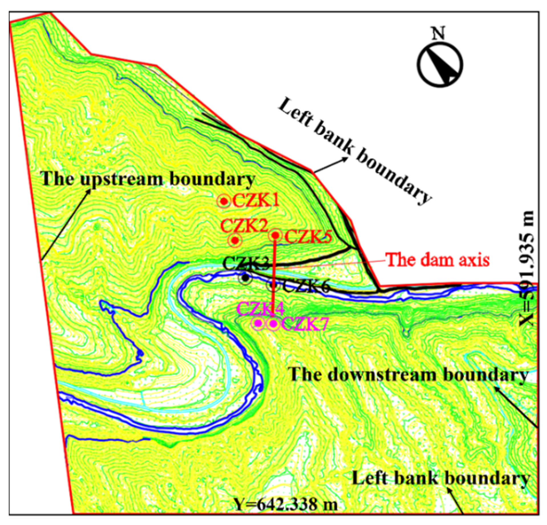
3.1. Basic Information on the Project Area

The reservoir of P hydropower station is a class III medium-sized reservoir. The pivotal project is composed of left and right bank water-retaining dam sections, riverbed overflow dam sections, bottom outlets, and water-intake dam sections. The dam is a roller-compacted concrete gravity dam with a maximum height of 59.50 m, a crest length of 217.00 m, and a crest width of 8 m. The normal storage and the design flood level of the reservoir are 946.5 m, the check flood level is 946.95 m, the total storage capacity is 15.81 × 10⁶ m³, and the backwater length is 6.082 km. The dam is a grade III structure, the design flood standard is a 50 year return period, and the corresponding peak flow is 808 m³/s; the check flood standard is a 500 year return period, and the corresponding peak discharge is 2110 m³/s. The seismic design intensity is VII.

The project area is located in a low hill and gully landscape with a high north and low south terrain; the river valley gully is relatively developed, and its cross-section is “U”-shaped. The main stratum of the project area is the Triassic Ermaying Formation. The lithology is mainly gray-green coarse-grained feldspathic sandstone, sandstone mudstone interbedding, siltstone, and silty mudstone. The rock stratum is stable and about 200 m thick. The stratum in the project area is divided into a strongly weathered, weakly weathered, and slightly new strata. The stratum is weakly permeable with good bottom sealing. The groundwater is mainly bedrock fissure phreatic water and quaternary pore phreatic water. Both reservoir banks are relatively wide and thick, without a thin watershed distribution, large structure, and fault distribution. Two groups of conjugate high-angle shear joints, NWW and NNE, are common, with a fracture spacing of 0.5~2.0 m.

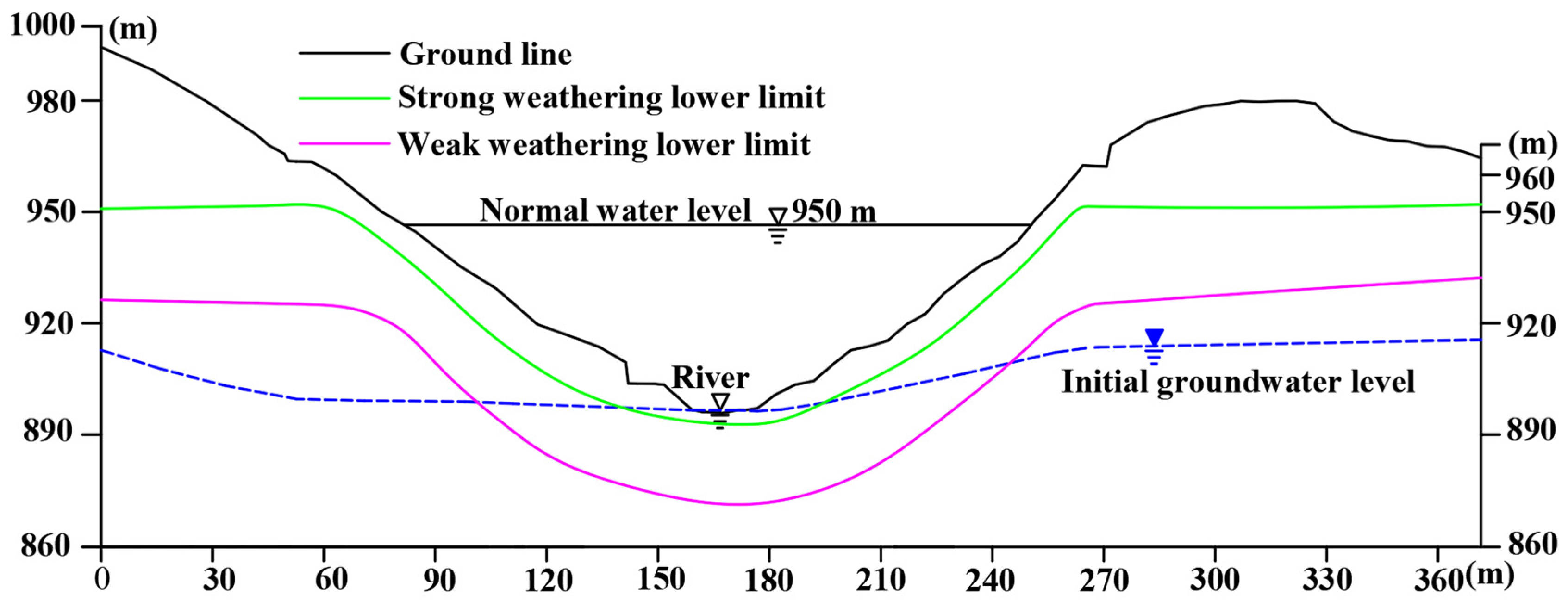
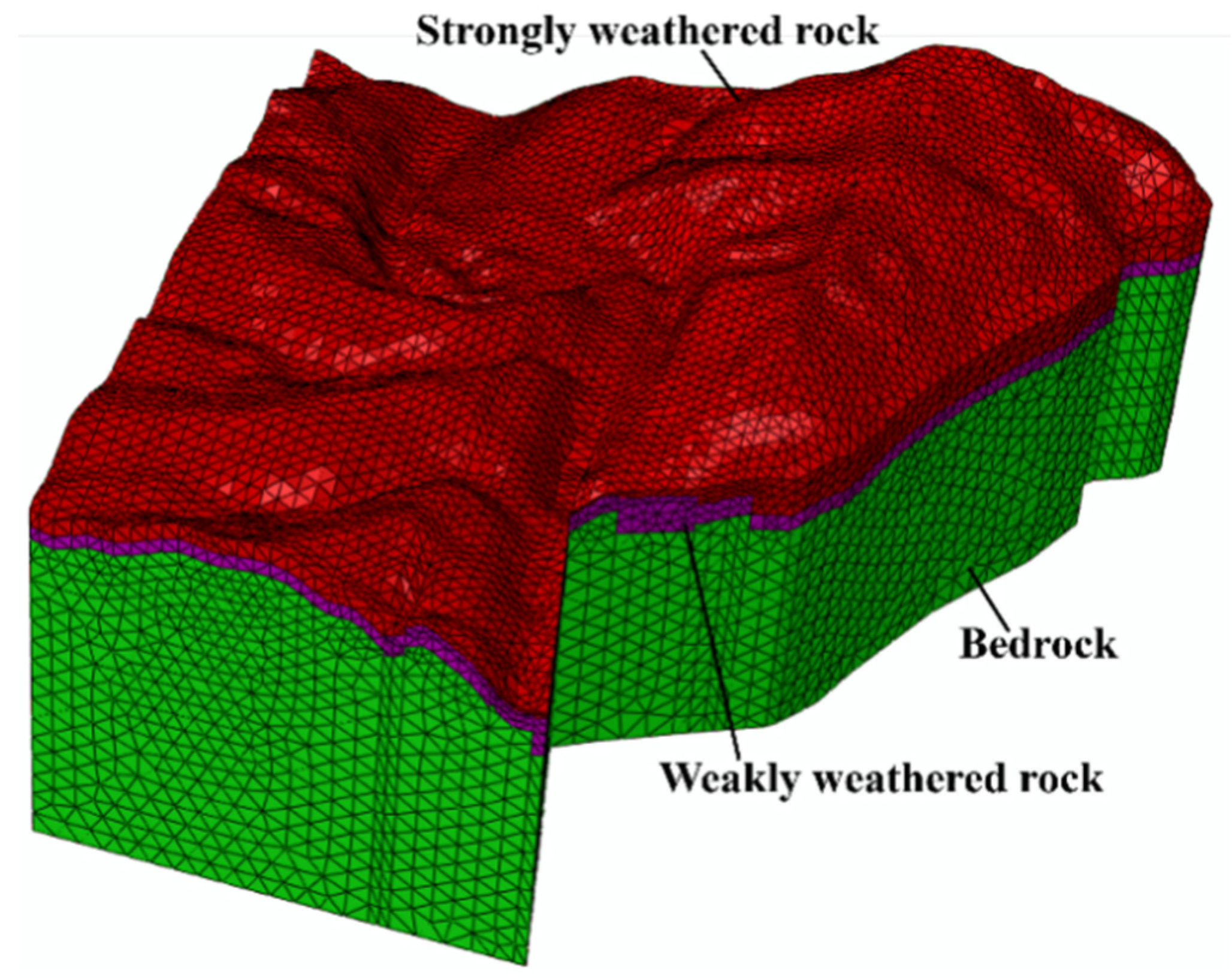
3.2. Establishment of the Finite Element Model

According to the geological survey report and relevant hydrogeological data, a three-dimensional finite element seepage model in the engineering area was established. The model’s boundary was determined by the seepage field and the site’s terrain. The surrounding was taken from the mountain watershed, and the thickness of the rock around the reservoir was not less than 3–5 times the dam height or the excavation span [31,32]. When the distance from the surface was less than five times the excavation span, it was calculated to the surface to ensure the rationality of the model calculation boundary. The upstream and downstream boundaries of the established model were 7.90 and 10.01 times the dam height from the dam site, respectively; the left and right boundaries were 3.79 and 9.29 times the dam height from the midpoint of the dam axis, respectively. Moreover, the left boundary was along the channel on the left bank of the downstream. Figure 2 shows the model’s scope, measuring 1284.67 m in length and 1183.87 m in width.

In order to make the calculation model consistent with the actual hydrogeological conditions in the project area, a detailed simulation of the strata located on both banks and the river valley was conducted on the basis of the geological profile of the dam axis, as illustrated in Figure 3. The thickness of the strongly and weakly weathered strata was 13.5 m and 24.2 m on the left bank, 3.9 m and 26.1 m on the river valley, and 3.8 m and 20.6 m on the right bank, respectively. Furthermore, the survey of adits on both banks revealed the presence of a wide fissure, measuring approximately 8 cm in width, and a long fissure, roughly 1.0 cm in width, on the right bank. On the left bank, a weak rock belt composed of sandy mudstone was observed, with a maximum thickness of 5 cm. These findings were simulated in the study.

In conclusion, the calculation model built using ABAQUS is shown in Figure 4. The bottom elevation of the model was 507.1 m, and the top elevation was the corresponding surface elevation. The four-node isoparametric element (C3D4P) was used to mesh the model. The numbers of nodes and units were 54,552 and 300,618, respectively. In the calculations, the right boundary, the left boundary, and the middle channel of the model used the measured groundwater level, the corresponding ditch bottom water level, and the natural river valley level as their constant water head boundaries, respectively; the upstream, downstream, and bottom were impermeable boundaries.

The study used the proposed inversion model to invert the dam foundation permeability coefficients of the P hydropower station using the measured water levels from seven boreholes (i.e., CZK1, CZK2, CZK3, CZK4, CZK5, CZK6, and CZK7) in the natural seepage field.

3.3. Sample Construction Based on Orthogonal Design

The permeability coefficient of various strata and fractures was an independent variable in the inversion. Since each stratum was mostly sandstone and mudstone interbedded with uneven lithology, their permeability coefficients were considered anisotropic. According to the geological survey data and combined with general engineering experience, the range of permeability coefficients was determined, as shown in

Table 1. Value range of permeability coefficients for each stratum and fracture.

Rock Stratum	Measured Range of k1 and k2 (m/s)	Measured Range of k3 (m/s)
Strongly weathered stratum	[4.32, 9.86] × 10−5	[1.12, 6.57] × 10−5
Weakly weathered stratum	[3.57, 9.25] × 10−6	[1.63, 7.49] × 10−6
Bedrock	[5.61, 8.94] × 10−7	[1.38, 4.67] × 10−7
Fracture	[5.35, 8.58] × 10−6	[1.24, 4.27] × 10−6

, where k₁ and k₂ are the tangential permeability coefficient values, and k₃ is the normal permeability coefficient value.

Constructing a reasonable permeability coefficient sample is crucial for developing a surrogate model. To ensure the RF model precision without increasing the workload of finite element forward analysis, this study adopted the orthogonal design method [33] to arrange a representative combination scheme of permeability coefficients. Orthogonal tables are essential to orthogonal test sample preparation. The scheme is generally expressed as L_n (t^c), where L is the orthogonal table, n is the total number of tests, t is the level number of factors, and c is the maximum number of factors arranged. The four factors of the test were the permeability coefficients of strongly weathered stratum, weakly weathered stratum, bedrock, and fracture.

Table 2. Values of parameters at different levels based on orthogonal design.

Level	Strongly Weathered Layer (×10−5 m/s)		Weakly Weathered Layer (×10−6 m/s)		Bedrock (×10−7 m/s)		Fissure (×10−6 m/s)
	k1 = k2	k3	k1 = k2	k3	k1 = k2	k3	k1 = k2	k3
1	4.32	1.12	3.57	1.63	5.61	1.38	5.35	1.24
2	5.01	1.80	4.28	2.36	6.03	1.79	5.75	1.62
3	5.71	2.48	4.99	3.10	6.44	2.20	6.16	2.00
4	6.40	3.16	5.70	3.83	6.86	2.61	6.56	2.38
5	7.09	3.85	6.41	4.56	7.28	3.03	6.97	2.76
6	7.78	4.53	7.12	5.29	7.69	3.44	7.37	3.13
7	8.48	5.21	7.83	6.03	8.11	3.85	7.77	3.51
8	9.17	5.89	8.54	6.76	8.52	4.26	8.18	3.89
9	9.86	6.57	9.25	7.49	8.94	4.67	8.58	4.27

shows each factor’s nine level numbers. The 81 permeability coefficient combination schemes were generated by SPSS using the orthogonal table L₈₁ (9⁴). Subsequently, the corresponding water head was determined through finite element forward analysis, and 81 sets of inversion samples were constructed. A total of 65 groups of samples (the first 80% of the data) were chosen for training the RF model, while 16 groups of samples (the remaining 20%) were used for verifying the model.

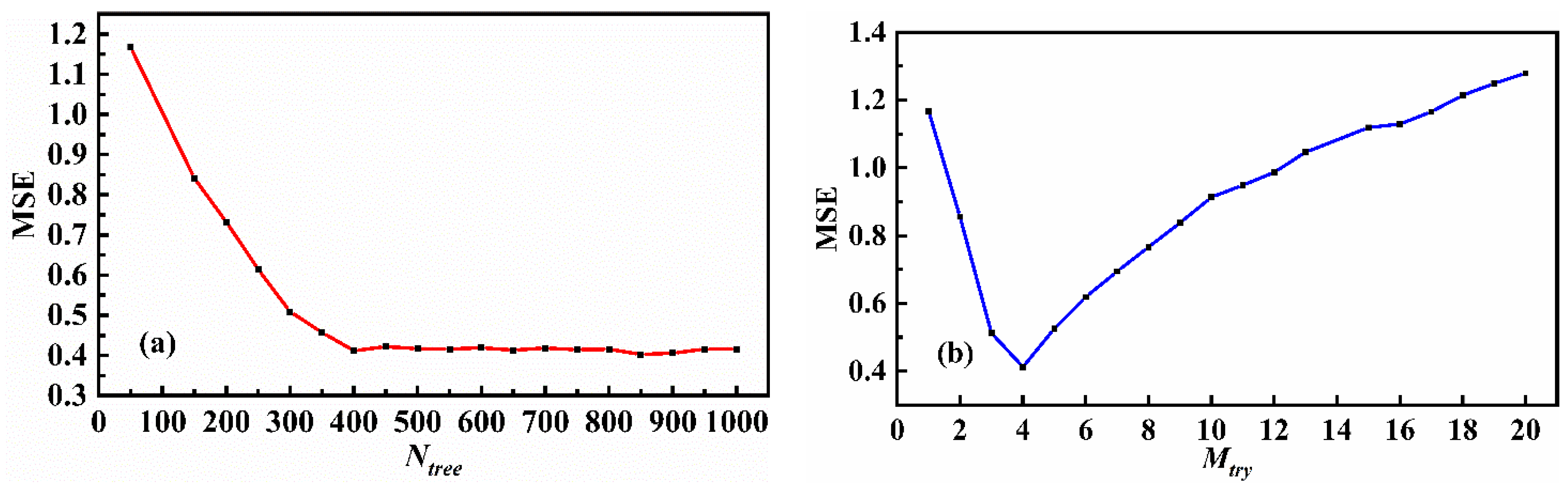
3.4. Determination of the RF Model Parameters

The establishment of the RF model relies heavily on setting the optimal Mtry and Ntree values, as demonstrated in Section 2.1. The variable control method was applied to analyze and determine RF parameter settings using the sample data from Section 3.3. The ideal RF parameters were selected using a tenfold cross-validation based on the model’s least MSE, effectively reducing model unpredictability.

To examine the model’s generalization ability under different N_tree, M_try was set to the default value (i.e., one-third of the number of variables), and the N_tree range was set to [50, 1000] with a step size of 50. Figure 5a depicts the model’s MSE change curve for different N_tree. It is evident that the model’s MSE stabilized when N_tree reached 400, indicating that increasing the number of model trees did not significantly affect the model error when M_try was fixed. Therefore, to enhance the computational efficiency and ensure the accuracy of the RF model, this study selected N_tree = 400. Subsequently, the model’s generalization ability was evaluated under different M_try levels, with N_tree set to 400 and M_try set to [1, 20] with a step size of 1. Figure 5a depicts the model’s MSE change curve for different M_try. It shows that the model’s MSE increased gradually with an increase in M_try, with the smallest MSE observed at M_try = 4. Accordingly, N_tree = 150 and M_try = 4 were identified as the optimal parameters for the RF model, leading to improved performance and computational efficiency.

4. Results and Analysis

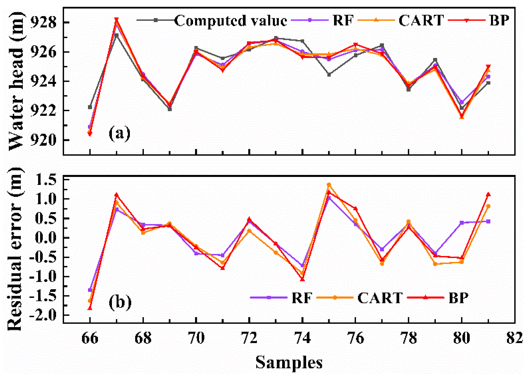
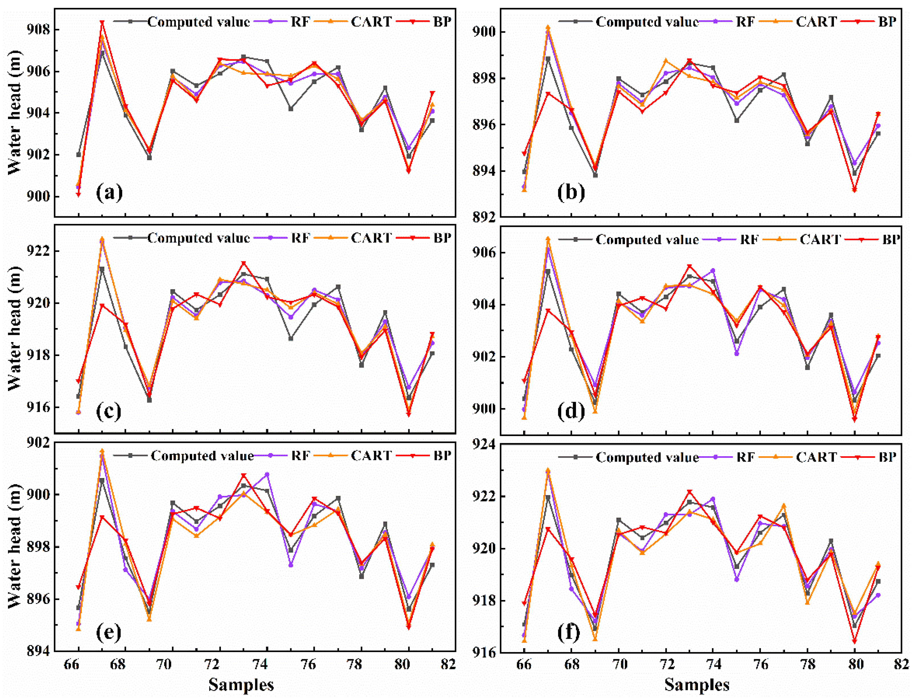
4.1. Performance Validation of the RF Model

The study evaluated the ability of the RF model to invert permeability parameters at borehole CZK1, comparing it to the CART model [18] and BP neural network model [19]. The RF model was configured with parameters N_tree and M_try set to 400 and 4, respectively; the CART model was configured with parameters minLeafSize and smoothingK set to 6 and 20, respectively; the BP model’s hidden layer consisted of seven neurons, and the maximum number of iterations was set to 200. Figure 6 displays the prediction results of the RF, CART, and BP models for the borehole water level.

Table 3. Evaluation indices of prediction results of RF, CART, and BP models at borehole CZK1.

Models	Model Training				Model Verification
	MAE (m)	MAPE (%)	RMSE (m)	R2	MAE (m)	MAPE (%)	RMSE (m)	R2
RF	0.290	0.031	0.353	0.962	0.255	0.055	0.589	0.879
CART	0.357	0.039	0.416	0.948	0.325	0.070	0.764	0.797
BP	0.385	0.042	0.457	0.937	0.695	0.075	0.827	0.762

presents the generalization ability and forecast accuracy of the three models according to different evaluation indices.

Figure 6a shows that the prediction curves of the three models were close to the finite element calculation curves, and the prediction errors were negligible. However, Figure 6b illustrates that the overall prediction residuals of the RF model were smaller than those of the CART and BP models. Table 3 proves that the RF model outperformed the CART and BP models in all evaluation indices. Notably, the R² values for the training and test sets were 0.962 and 0.879, respectively, and other indices also achieved low values, indicating that the RF model fit was highly significant. Consequently, the prediction accuracy of the RF model was higher, and the proxy model based on the RF model accurately predicted the water head of borehole CZK1.

The water heads of boreholes CZK2, CZK3, CZK4, CZK5, CZK6, and CZK7 were utilized to assess the generalization ability of the RF model. Figure 7 illustrates the water head prediction results of the RF, CART, and BP models at these boreholes.

Table 4. Evaluation indices of prediction results of RF, CART, and BP models at different boreholes.

Measuring Points	Models	Model Training				Model Verification
		MAE (m)	MAPE (%)	RMSE (m)	R2	MAE (m)	MAPE (%)	RMSE (m)	R2
CZK2	RF	0.304	0.034	0.366	0.960	0.262	0.058	0.626	0.864
	CART	0.366	0.041	0.430	0.944	0.341	0.075	0.764	0.797
	BP	0.385	0.043	0.457	0.937	0.844	0.093	0.967	0.675
CZK3	RF	0.339	0.038	0.413	0.948	0.241	0.054	0.543	0.898
	CART	0.373	0.042	0.437	0.942	0.338	0.075	0.724	0.818
	BP	0.388	0.043	0.449	0.939	0.687	0.077	0.755	0.802
CZK4	RF	0.326	0.035	0.377	0.957	0.252	0.055	0.548	0.896
	CART	0.362	0.039	0.405	0.951	0.294	0.064	0.635	0.860
	BP	0.419	0.046	0.477	0.931	0.672	0.073	0.745	0.807
CZK5	RF	0.339	0.038	0.379	0.957	0.221	0.049	0.473	0.922
	CART	0.362	0.040	0.407	0.950	0.280	0.062	0.609	0.871
	BP	0.422	0.047	0.453	0.938	0.633	0.070	0.688	0.836
CZK6	RF	0.350	0.039	0.384	0.955	0.242	0.054	0.510	0.909
	CART	0.426	0.047	0.449	0.939	0.285	0.063	0.610	0.869
	BP	0.482	0.054	0.516	0.920	0.626	0.070	0.669	0.844
CZK7	RF	0.403	0.044	0.452	0.938	0.224	0.049	0.475	0.922
	CART	0.406	0.044	0.424	0.946	0.250	0.054	0.527	0.903
	BP	0.471	0.051	0.490	0.927	0.587	0.064	0.617	0.868

presents a quantitative evaluation of the prediction results.

Figure 7 indicates that the RF model outperformed the other two models regarding anti-interference and generalization. Specifically, the RF model’s R² values at boreholes CZK2, CZK3, CZK4, CZK5, CZK6, and CZK7 were 0.864, 0.898, 0.896, 0.922, 0.909, and 0.922, respectively, which were superior to those of the CART (R² = 0.797, 0.818, 0.860, 0.871, 0.869, and 0.903) and BP (R² = 0.675, 0.802, 0.807, 0.836, 0.844, and 0.868) models, as reported in Table 4. Moreover, the other statistical indices of the RF model outperformed those of the CART and BP models, indicating its excellent generalization ability. Overall, the RF model accurately predicted the water head at all seven boreholes, making it a suitable surrogate model for inverting engineering seepage parameters with high accuracy and robustness.

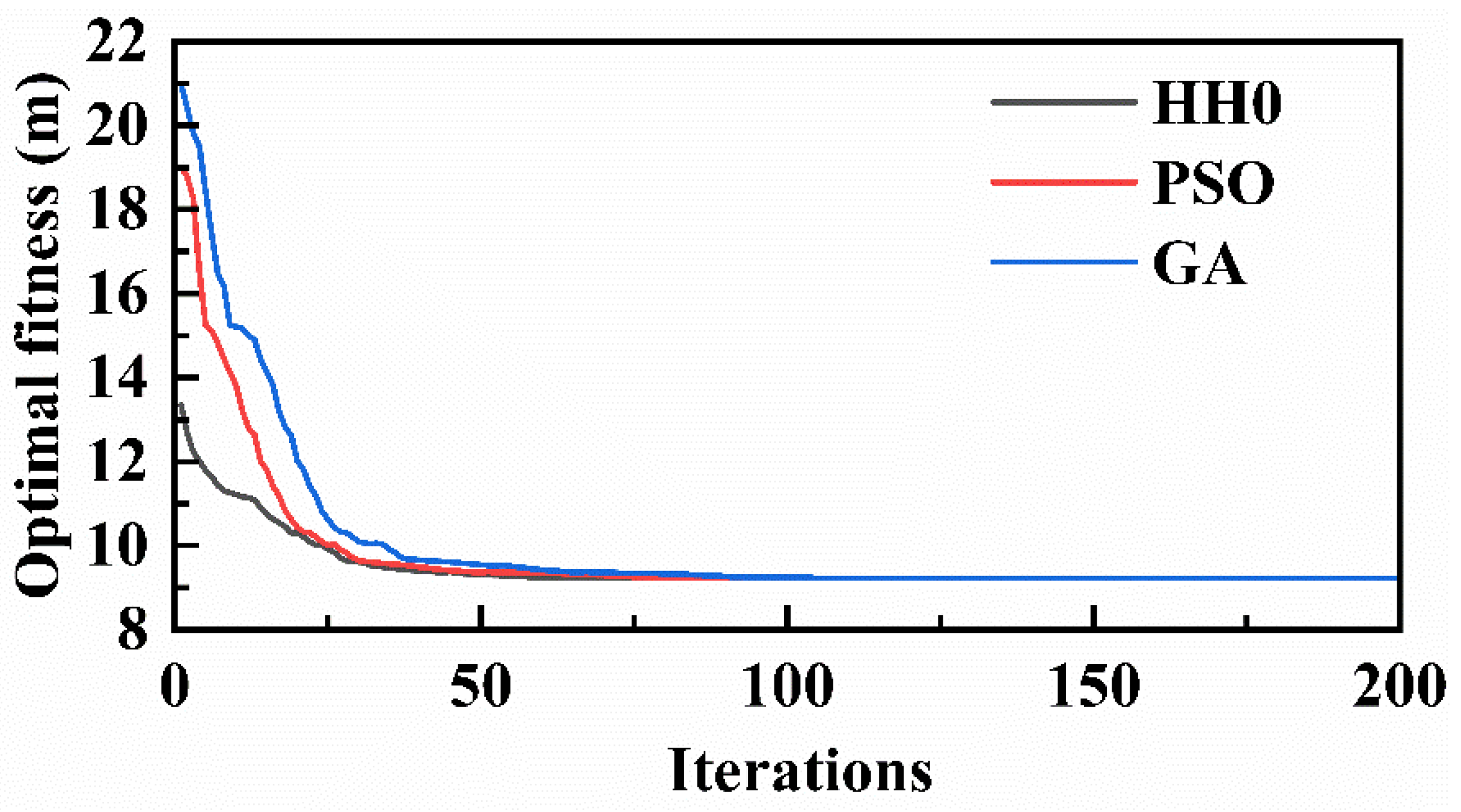
4.2. Inversion of Permeability Coefficients Based on the HHO Algorithm

Section 4.1 verified that the constructed surrogate model predicted borehole water heads well. Utilizing this model, the HHO algorithm was employed in global optimization within the range of permeability coefficients (i.e., Table 1). The initial number of hawks was set to N = 50, the maximum number of iterations was T = 200, and the fitness value was calculated using the trained RF in Section 4.1. To validate the HHO algorithm’s optimization capacity, classic optimization algorithms such as the genetic algorithm (GA) [34] and PSO [35] were introduced for comparison. During calculation, the PSO algorithm’s parameters were set to 100 for the number of particle swarms, 1.5 for the individual learning factor, 2 for the social learning factor, 1 for the maximum inertia factor, 0.8 for the minimum inertia factor, and 200 for the maximum number of iterations. The GA algorithm’s parameters were set to 100 for the population size, 0.85 for the generation gap, 0.6 for the crossover probability, 0.01 for the mutation probability, and 200 for the maximum genetic algebra. Figure 8 illustrates the convergence process of the HHO, PSO, and GA algorithms in searching for the optimal solution.

Figure 8 illustrates that the HHO algorithm exhibited a smoother convergence curve, a superior initial optimization result, and a faster convergence rate than the PSO and GA algorithms. The HHO, PSO, and GA algorithms achieved optimal results at the 66th, 96th, and 105th generations, respectively. The convergence rates of all three algorithms were relatively flat, indicating their strong global search capabilities. However, the HHO algorithm required fewer initial parameters, with only N and T needing to be determined, thus simplifying programming.

Table 5. Inversion results of permeability coefficient of each stratum and fracture.

Rock Stratum	Calculated Value of k1 and k2 (m/s)	Calculated Value of k3 (m/s)
Strongly weathered stratum	8.43 × 10−5	5.47 × 10−5
Weakly weathered stratum	7.81 × 10−6	6.14 × 10−6
Bedrock	7.46 × 10−7	3.69 × 10−7
Fracture	7.29 × 10−6	2.87 × 10−6

presents the optimal permeability coefficient for each stratum and fracture.

To confirm the validity of the permeability coefficient obtained, we applied the inverted permeability coefficients of each stratum and fracture to the FEM. This allowed us to calculate the water head of each borehole and compare it with the measured water level. The results are presented in

Table 6. Comparison of measured and inverted water levels at each borehole.

Borehole	Calculated Water Level (m)	Measured Water Level (m)	Absolute Error (m)	Relative Error (%)
CZK1	920.83	928.74	−7.91	0.85
CZK2	905.67	902.24	3.43	0.38
CZK3	899.83	895.97	3.86	0.43
CZK4	922.75	912.62	10.13	1.11
CZK5	904.56	899.64	4.92	0.55
CZK6	898.32	895.84	2.48	0.28
CZK7	921.41	913.51	7.90	0.87

. The calculation formulas for absolute error e and relative error e_r are presented in Equations (21) and (22), respectively:

$$e=H^{\prime }-H,$$

(21)

$$e_{\mathrm{r}}=\left[(H^{\prime }-H)/H\right]\times 100\%,$$

(22)

where $H^{\prime }$ and $H$ are the calculated and measured water levels of the borehole, respectively.

Several studies [3,31,32] suggested that the inverted permeability coefficient is suitable when e < 10 m and e_r < 5% at each borehole. Table 6 shows that CZK4 had the highest absolute error of 10.13 m and the highest relative error of 1.11%, while the remaining boreholes had minor absolute and relative errors that met the accuracy control requirements. The disparity between the calculated and measured water level at CZK4 was due to a decline in the groundwater level caused by the construction of the exploration adit near the borehole, which resulted in a significant difference between the measured and true water level for the borehole. Therefore, in future research, the borehole water level must be corrected near the adit, or one should avoid using similar borehole information before inversion. However, the disparity between the calculated and measured water level in the remaining boreholes was slight, indicating that the geological permeability coefficient inverted was close to its true value, and the seepage properties of the project area calculated could be used as its natural seepage field distribution. In conclusion, the permeability coefficients obtained using the RF–HHO model met the project’s requirements for accuracy. They can be applied to analyze and calculate seepage properties under different situations during the construction and operation of the project area.

For seepage calculation analysis, X = 591.935 m and Y = 642.335 m in the calculation model were used as typical profiles, as shown in Figure 2. Figure 9 and Figure 10 show the total water head and pressure water head distribution calculated for the two profiles. The left and right banks of the X profile are the upstream and downstream, respectively; the left and right of the Y profile are the right and left banks, respectively.

The results indicated that the upstream reservoir area of the initial seepage field exhibited a higher water head than the downstream area, validating the principle of seepage supplement from upstream to downstream. The upstream water head line was distributed more densely, and the hydraulic gradient was relatively large. Similarly, the water head on the right side of the initial seepage field model was higher than the left side, indicating the law of seepage supplement from the mountain to the river valley. The water head line was distributed more densely on the right side, and the hydraulic gradient was relatively large. The distribution pattern of the initial seepage field computed aligned with the pattern revealed by the borehole, which was consistent with the distribution law of the general mountain seepage field. Moreover, the distribution of the total head and pore water pressure was essentially reasonable.

5. Conclusions

The geological permeability coefficient is a critical parameter in hydraulic engineering for analyzing the safety of three-dimensional seepage fields. However, estimating its actual value is a challenge due to the interaction of various elements. Therefore, it is crucial to establish a high-precision model to quickly obtain the permeability coefficient’s “true value”. In this study, we applied an RF–HHO-based model for permeability coefficient inversion to the dam foundation of the P hydropower station, which revealed the overall distribution characteristics of its natural seepage field. On the basis of our research, we can draw the following conclusions:

(1)

The RF model showed promising potential for engineering seepage parameter inversion. Compared to other models, the RF model’s water level prediction at all boreholes was closer to the calculated value of the FEM, with its evaluation index being the smallest, indicating its greater prediction accuracy and generalization ability. The RF-based surrogate model can replace the FEM for seepage calculation, avoiding the time-consuming process of FEM seepage calculation and improving the efficiency of the inversion process.

(2)

The HHO algorithm demonstrated remarkable proficiency in conducting global searches. As evidenced by the convergence curve of parameter optimization, the HHO method surpassed the PSO and GA algorithms regarding optimization efficiency and initial setting parameters. It could rapidly identify the optimal solution by determining the population and maximum iterations.

(3)

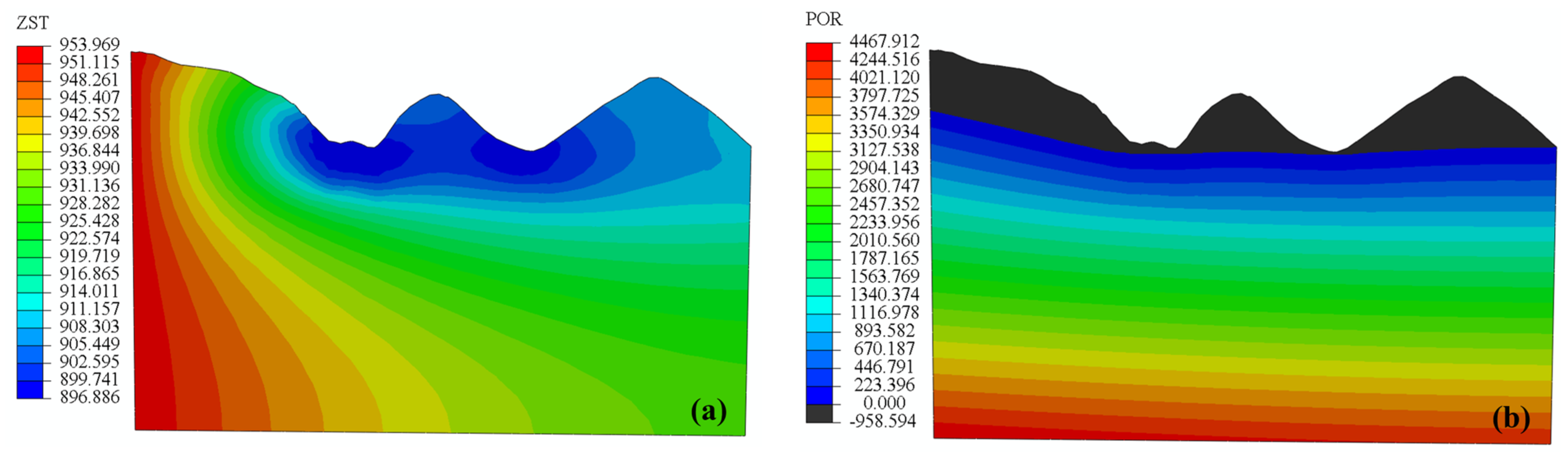
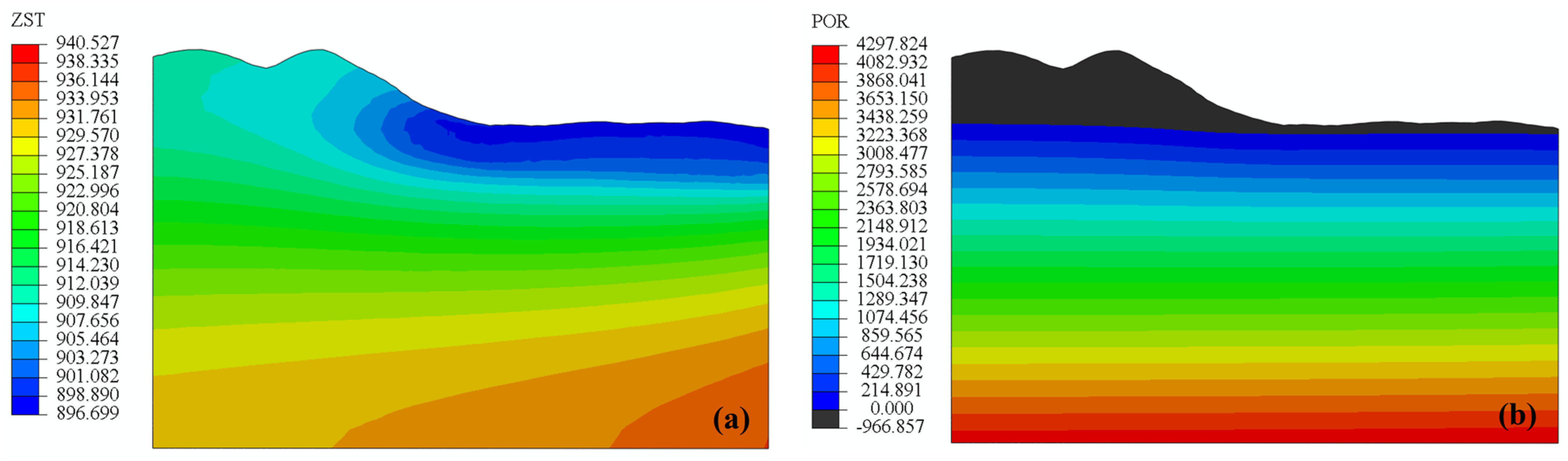
The inversion model constructed provided a solid foundation for the numerical study of the natural seepage field in the project area. The RF–HHO model successfully determined the optimal permeability coefficient of the geology for the P hydropower station, and then calculated the water head for each borehole using FEM. The absolute and relative errors between the calculated and measured water levels in the borehole were small. Additionally, the calculated distribution pattern of the initial seepage field was consistent with the distribution law of the mountain seepage field. These results indicate that the inversion model was reasonable and met the engineering requirements for accuracy.

However, it is a deficiency that the study only used single-borehole data modeling to invert the optimum permeability coefficient for the geology without considering the linkage between different boreholes. Boreholes are frequently situated near one another and possess interrelated characteristics that can be utilized for parametric inversion modeling. As such, our forthcoming research endeavors will maximize the linkages between the different boreholes to enhance the current model.

References

1. Mao, X.; Pan, S.; Bai, Z. Back analysis of initial seepage field of complex dam foundation at Shuangjiangkou Hydropower Station. Rock Soil Mech. 2008, 29 (Suppl. S1), 135–139. [Google Scholar]
2. Dong, W.; Yuan, H.; Xu, W.; Zhang, B.; Yu, Y. Dynamic back-analysis of material parameters of Nuozhadu high earth-rock-fill dam. J. Hydroelectr. Eng. 2012, 31, 203–208. [Google Scholar]
3. Xu, Z.; Cao, C.; Li, K.; Junrui, C. Analysis of part seepage control scheme of an upper reservoir of a pumped-storage power station. Chin. J. Appl. Mech. 2018, 35, 417–422+459. [Google Scholar]
4. Mao, C. Seepage Calculation, Analysis and Control; Water Resources and Electric Power Press: Beijing, China, 1990. [Google Scholar]
5. Sheng, J.; Su, B.; Zhan, M. Back analysis of 3d seepage problem and its engineering application. Chin. J. Rock Mech. Eng. 2003, 22, 203–207. [Google Scholar]
6. Zhu, B. A new method for the back analysis of seepage problem. J. Hydraul. Eng. 1994, 39, 42–46. [Google Scholar]
7. Duan, B.; Zhang, L.; He, J.; Fu, W.; Chen, G. Back analysis of natural seepage field in complicated fractured rock mass. J. Hydroelectr. Eng. 2012, 31, 188–193. [Google Scholar]
8. Lu, P.; Wang, X.; Wu, B.; Cheng, Z. Seepage parameter inversion based on Bayesian theory and entropy-blind numbers. J. Hydroelectr. Eng. 2019, 38, 108–118. [Google Scholar]
9. Chi, S.; Ni, S.; Liu, Z. Back analysis of the permeability coefficient of a high core rockfill dam based on a RBF neural network optimized using the PSO algorithm. Math. Probl. Eng. 2015, 2015, 124042. [Google Scholar] [CrossRef]
10. Xu, L.; Shen, Z. Inversion model of permeability coefficient for complex earth rock dam based on ELM-GA. Water Resour. Power 2021, 39, 86–90. [Google Scholar]
11. Tang, S.; Xiong, W.; Wan, X.; Luo, Z.; Wan, S.; Wang, Q. Multi-objective inversion analysis method for dam permeability coefficient based on GA-BP. China Rural. Water Hydropower 2020, 62, 213–216. [Google Scholar]
12. Chen, H.; Teng, Y.; Wang, J. Methods of estimation of hydraulic conductivity with genetic algorithm-support vector regression machine. Hydrogeol. Eng. Geol. 2011, 38, 14–18. [Google Scholar]
13. Yu, H.; Wang, X.; Ren, B.; Zeng, T.; Lv, M.; Wang, C. An efficient Bayesian inversion method for seepage parameters using a data-driven error model and an ensemble of surrogates considering the interactions between prediction performance indicators. J. Hydrol. 2022, 604, 127235. [Google Scholar] [CrossRef]
14. Ni, S.; Chi, S. Back analysis of permeability coefficient of high core rockfill dam based on particle swarm optimization and support vector machine. Chin. J. Geotech. Eng. 2017, 39, 727–734. [Google Scholar]
15. Li, Y.; Yang, J.; Cheng, L.; Ma, C. Inversion Analysis on Permeability Coefficient of Stratum in Engineering Area Based on RVM-CS. J. Yangtze River Sci. Res. Inst. 2020, 37, 121–127. [Google Scholar]
16. Shu, Y.; Shen, Z.; Xu, L.; Zhang, K.; Yang, C. Inversion analysis of impervious curtain permeability coefficient using calcium leaching model, extreme learning machine, and optimization algorithms. Appl. Sci. 2022, 12, 3272. [Google Scholar] [CrossRef]
17. Breiman, L. Random forests. Mach. Learn. 2001, 45, 5–32. [Google Scholar] [CrossRef]
18. Chen, X.; Zhao, X.; Tahmasebi, P.; Luo, C.; Cai, J. NMR-data-driven prediction of matrix permeability in sandstone aquifers. J. Hydrol. 2023, 618, 129147. [Google Scholar] [CrossRef]
19. Zhao, X.; Chen, X.; Huang, Q.; Lan, Z.; Wang, X.; Yao, G. Logging-data-driven permeability prediction in low-permeable sandstones based on machine learning with pattern visualization: A case study in Wenchang A Sag, Pearl River Mouth Basin. J. Pet. Sci. Eng. 2022, 214, 110517. [Google Scholar] [CrossRef]
20. Heidari, A.; Mirjalili, S.; Faris, H.; Aljarah, I.; Mafarja, M.; Chen, H. Harris hawks optimization: Algorithm and applications. Future Gener. Comput. Syst. 2019, 97, 849–872. [Google Scholar] [CrossRef]
21. Yu, J.; Kim, C.H.; Rhee, S.B. The comparison of lately proposed Harris hawks optimization and jaya optimization in solving directional overcurrent relays coordination problem. Complexity 2020, 2020, 3807653. [Google Scholar] [CrossRef]
22. Abbasi, A.; Firouzi, B.; Sendur, P. On the application of Harris hawks optimization (HHO) algorithm to the design of microchannel heat sinks. Eng. Comput. 2021, 37, 1409–1428. [Google Scholar] [CrossRef]
23. Li, Y.; Yin, Q.; Zhang, Y.; Qiu, W. Prediction of long-term maximum settlement deformation of concrete face rockfill dams using hybrid support vector regression optimized with HHO algorithm. J. Civ. Struct. Health Monit. 2023, 13, 371–386. [Google Scholar] [CrossRef]
24. Malik, A.; Tikhamarine, Y.; Sammen, S.S.; Abba, S.I.; Shahid, S. Prediction of meteorological drought by using hybrid support vector regression optimized with HHO versus PSO algorithms. Environ. Sci. Pollut. Res. 2021, 28, 39139–39158. [Google Scholar] [CrossRef] [PubMed]
25. Moayedi, H.; Osouli, A.; Nguyen, H.; Rashid, A.S.A. A novel Harris hawks’ optimization and k-fold cross-validation predicting slope stability. Eng. Comput. 2021, 37, 369–379. [Google Scholar] [CrossRef]
26. Bui, D.T.; Moayedi, H.; Kalantar, B.; Osouli, A.; Pradhan, B.; Nguyen, H.; Rashid, A.S.A. Harris hawks optimization: A novel swarm intelligence technique for spatial assessment of landslide susceptibility. Sensors 2019, 19, 3590. [Google Scholar] [CrossRef] [PubMed]
27. Xu, K.; Lei, X.; Meng, Q. Application of seepage back analysis to a hydropower engineering. Eng. J. Wuhan Univ. 2011, 44, 37–39. [Google Scholar]
28. Barati, R. Application of excel solver for parameter estimation of the nonlinear Muskingum models. KSCE J. Civ. Eng. 2013, 17, 1139–1148. [Google Scholar] [CrossRef]
29. Hosseini, K.; Nodoushan, E.J.; Barati, R.; Shahheydari, H. Optimal design of labyrinth spillways using meta-heuristic algorithms. KSCE J. Civ. Eng. 2016, 20, 468–477. [Google Scholar] [CrossRef]
30. Alizadeh, M.J.; Shahheydari, H.; Kavianpour, M.R.; Shamloo, H.; Barati, R. Prediction of longitudinal dispersion coefficient in natural rivers using a cluster-based Bayesian network. Environ. Earth Sci. 2017, 76, 86. [Google Scholar] [CrossRef]
31. Sun, C.; Chai, J.; Xu, Z.; Qin, Y. Numerical simulation and assessment of seepage control effects on surrounding fractured rocks of underground powerhouse in Jinchuan Hydropower Station. Chin. J. Geotech. Eng. 2016, 38, 786–797. [Google Scholar]
32. Xu, Z.; Liu, Y.; Huang, J.; Wen, L. Performance assessment of the complex seepage control system at the LuDila hydropower station in China. Int. J. Geomech. 2019, 19, 05019001. [Google Scholar] [CrossRef]
33. Li, Y.; Li, S.; Ding, Z.; Tu, X. The sensitivity analysis of Duncan-Chang E-B model parameters based on the orthogonal test method. J. Hydraul. Eng. 2013, 44, 873–879. [Google Scholar]
34. Haupt, R.L.; Haupt, S.E. Practical Genetic Algorithms; John Wiley & Sons: Hoboken, NJ, USA, 2004. [Google Scholar]
35. Mirjalili, S.; Dong, J.; Lewis, A.; Sadiq, A.S. Particle swarm optimization: Theory, literature review, and application in airfoil design. In Nature-Inspired Optimizers; Springer: Berlin/Heidelberg, Germany, 2020; pp. 167–184. [Google Scholar]
Figure 1. Execution process of the inversion model of the geological permeability coefficient.
Water 15 01993 g001
Figure 2. Calculation scope of seepage inversion analysis model in the project area.
Water 15 01993 g002
Figure 3. Engineering geological profile of dam axis at dam site.
Water 15 01993 g003
Figure 4. The inversion calculation model of the seepage field.
Water 15 01993 g004
Figure 5. The effect of the parameters on RF model performance: (a) Ntree, and (b) Mtry.
Water 15 01993 g005
Figure 6. Model accuracy verification results at borehole CZK1: (a) water head, and (b) residuals.
Water 15 01993 g006
Figure 7. Model accuracy verification results at different boreholes: (a) CZK2, (b) CZK3, (c) CZK4, (d) CZK5, (e) CZK6, and (f) CZK7.
Water 15 01993 g007
Figure 8. Convergence process of HHO, PSO, and GA algorithms.
Water 15 01993 g008
Figure 9. Calculation results of Y = 642.335 m profile (unit/m): (a) total water head, and (b) pore water pressure.
Water 15 01993 g009
Figure 10. Calculation results of X = 591.935 m profile (unit/m): (a) total water head, and (b) pore water pressure.
Water 15 01993 g010