
A Novel Early Warning System (EWS) for Water Quality, Integrating a High-Frequency Monitoring Database with Efficient Data Quality Control Technology at a Large and Deep Lake (Lake Qiandao), China

 , ,
, ,
Abstract
:1. Introduction
2. Methodology
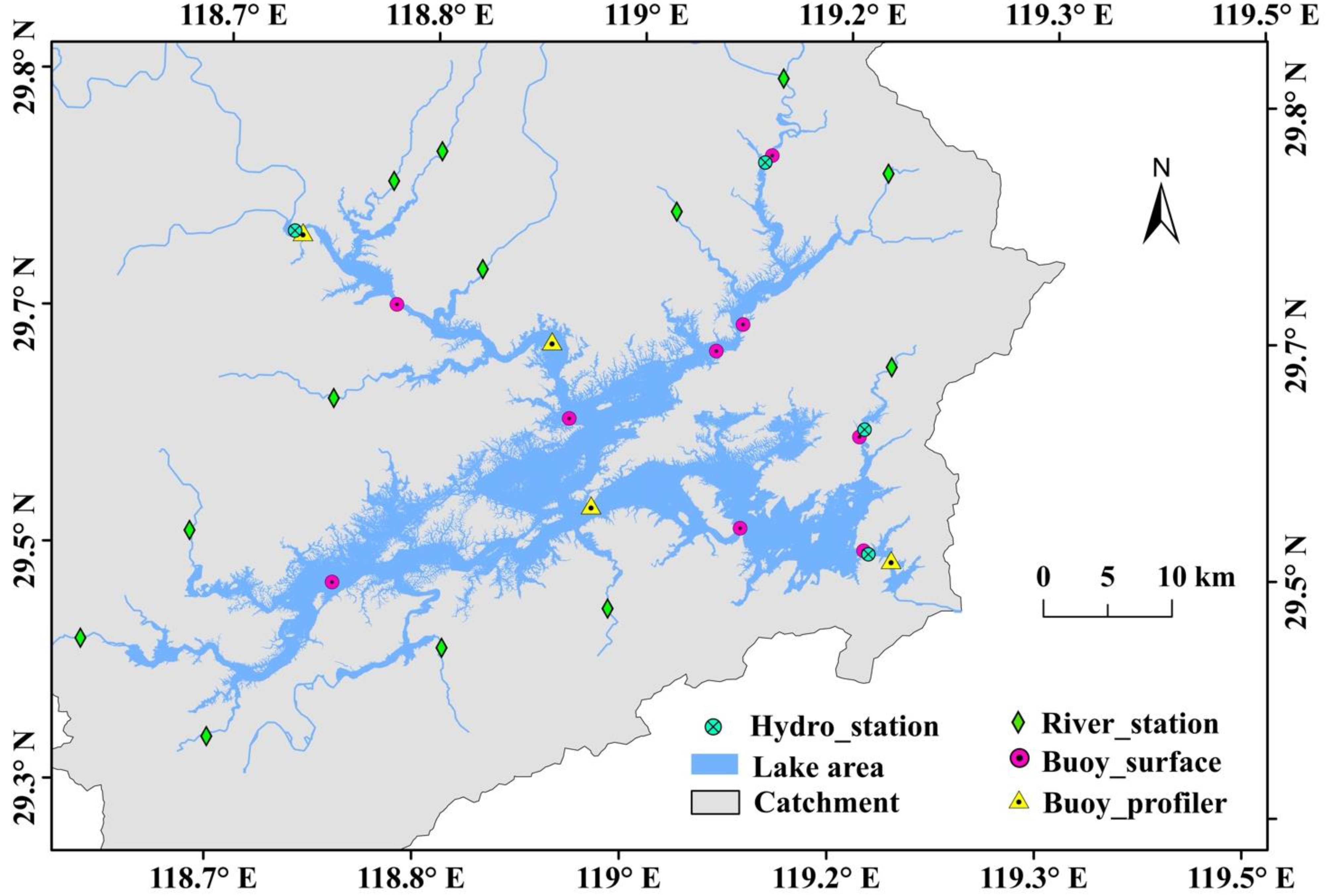
2.1. Study Area
2.2. Monitoring Stations
2.3. Sensor Information and Alert Range
2.4. Data Quality Control
2.5. Change Point and Trend Detections
2.6. Data Availability, Daily and Hourly Data Calculation
3. Results
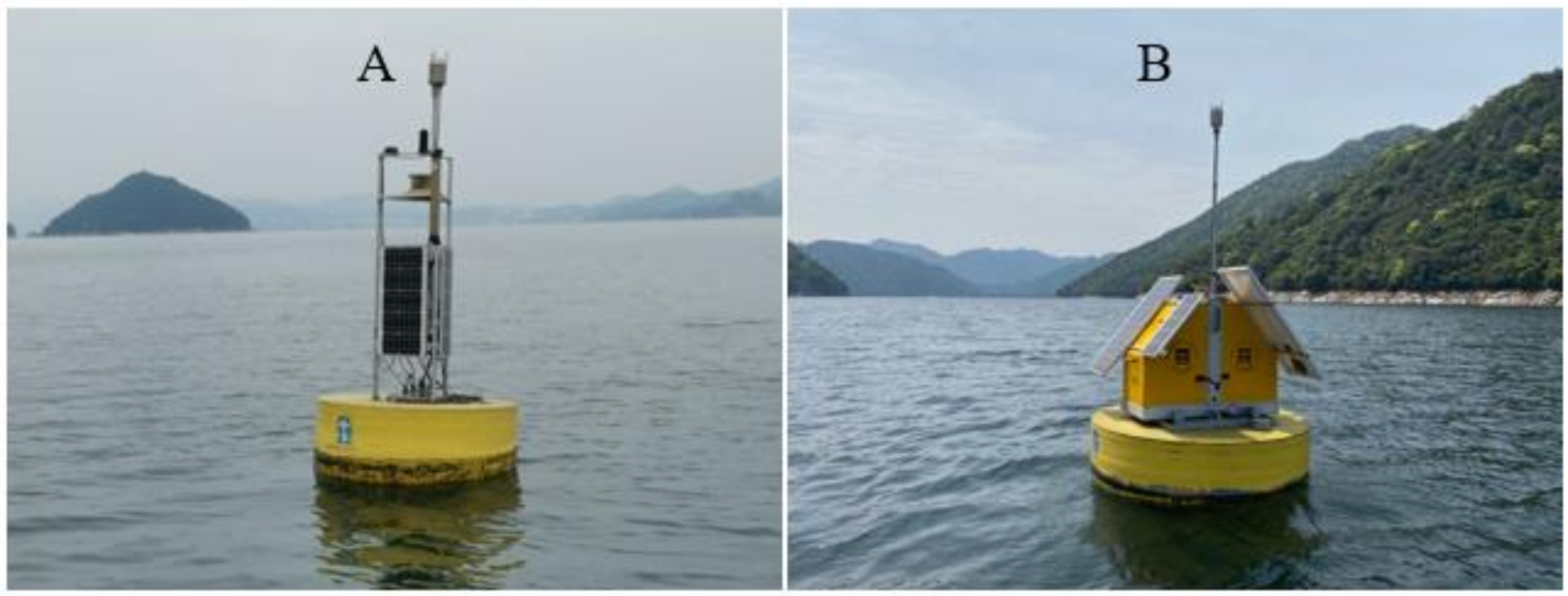
3.1. Buoy Photographs
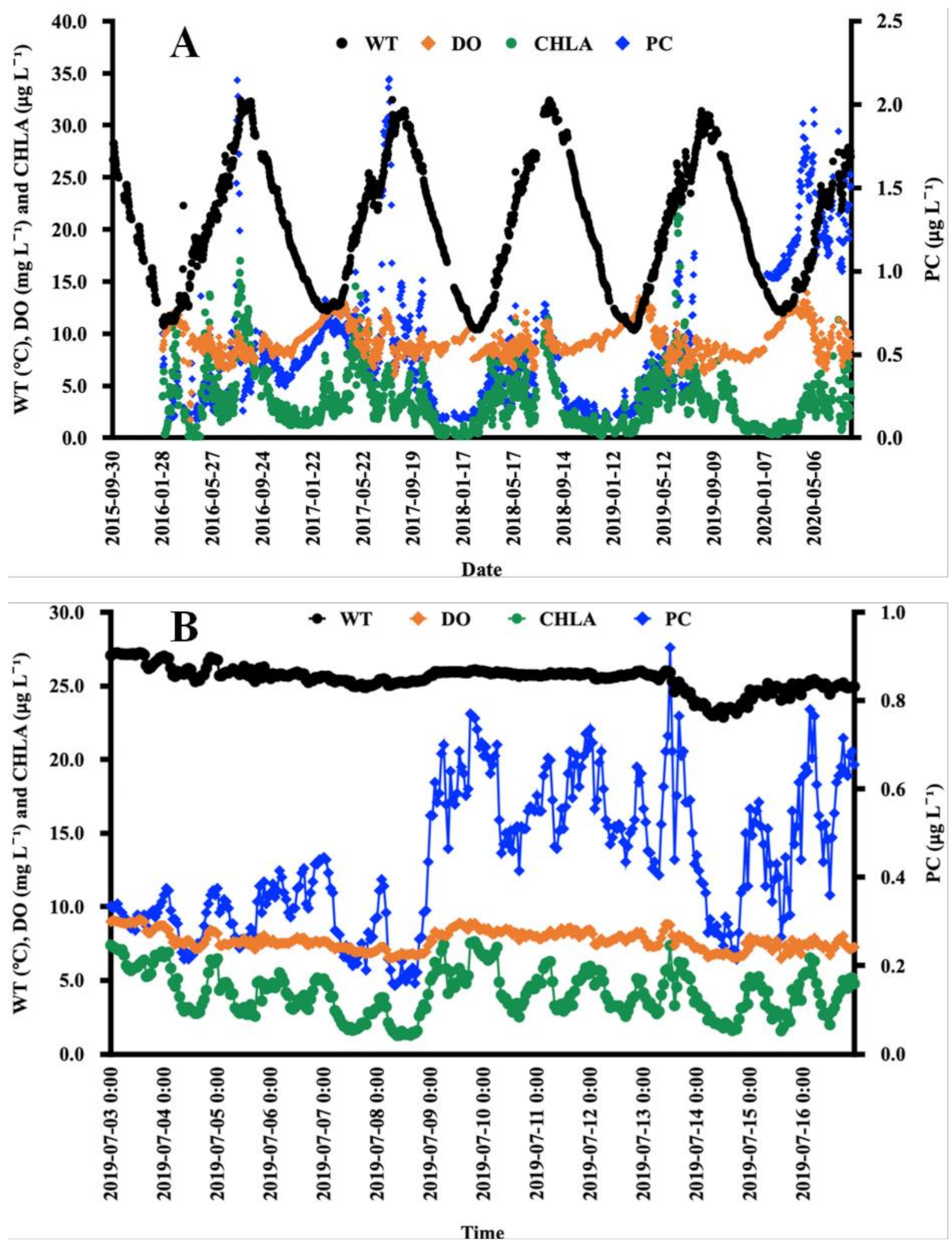
3.2. Surface Measurements
3.3. Profiling Measurements
3.4. Real-Time Early Warning Information
4. Discussion
Author Contributions
Funding
Institutional Review Board Statement
Informed Consent Statement
Acknowledgments
Conflicts of Interest
References
- Greeson, P.E. Lake eutrophication—A natural process. J. Am. Water Resour. Assoc. 1969, 5, 16–30. [Google Scholar] [CrossRef]
- Anderson, D.M.; Glibert, P.M.; Burkholder, J.M. Harmful algal blooms and eutrophication: Nutrient sources, composition, and consequences. Estuaries 2002, 25, 704–726. [Google Scholar] [CrossRef]
- Smith, V.H.; Schindler, D.W. Eutrophication science: Where do we go from here? Trends Ecol. Evol. 2009, 24, 201–207. [Google Scholar] [CrossRef]
- Conley, D.J.; Paerl, H.W.; Howarth, R.W.; Boesch, D.F.; Seitzinger, S.P.; Havens, K.E.; Lancelot, C.; Likens, G.E. Controlling eutrophication: Nitrogen and phosphorus. Sciences 2009, 323, 1014–1015. [Google Scholar] [CrossRef]
- Lee, J.H.W.; Hodgkiss, I.J.; Wong, K.T.M.; Lam, I.H.Y. Real time observations of coastal algal blooms by an early warning system. Estuar. Coast. Shelf Sci. 2005, 65, 172–190. [Google Scholar] [CrossRef]
- Wang, X.; Su, J.; Cai, Y.; Tan, Y.; Yang, Z.; Wang, F. An integrated approach for early warning of water stress in shallow lakes: A case study in Lake Baiyangdian, North China. Lake Reserv. Manag. 2013, 29, 285–302. [Google Scholar] [CrossRef] [Green Version]
- Burchard-Levine, A.; Liu, S.; Vince, F.; Li, M.; Ostfeld, A. A hybrid evolutionary data driven model for river water quality early warning. J. Environ. Manag. 2014, 143, 8–16. [Google Scholar] [CrossRef]
- Park, Y.; Cho, K.H.; Park, J.; Cha, S.M.; Kim, J.H. Development of early-warning protocol for predicting chlorophyll-a concentration using machine warning models in freshwater and estuarine reservoirs, Korea. Sci. Total Environ. 2015, 502, 31–41. [Google Scholar] [CrossRef]
- Biddanda, B.A.; Weinke, A.D.; Kendall, S.T.; Gereaux, L.C.; Holcomb, T.M.; Snider, M.J.; Dila, D.K.; Long, S.A.; VandenBerg, C.; Knapp, K.; et al. Chronicles of hypoxia: Time-series buoy observations reveal annually recurring seasonal basin-wide hypoxia in Muskegon Lake—A Great Lakes estuary. J. Great Lakes Res. 2018, 44, 219–229. [Google Scholar] [CrossRef]
- Delpla, I.; Florea, M.; Rodriguez, M.J. Drinking water source monitoring using early warning systems based on data mining techniques. Water Resour. Manag. 2019, 33, 129–140. [Google Scholar] [CrossRef]
- Glasgow, H.B.; Burkholder, J.M.; Reed, R.E.; Lewitus, A.J.; Kleinman, J.E. Real-time remote monitoring of water quality: A review of current applications, and advancements in sensor, telemetry, and computing technologies. J. Exp. Mar. Biol. Ecol. 2004, 300, 409–448. [Google Scholar] [CrossRef]
- Ungureanu, F.; Lupu, R.G.; Stan, A.; Craciun, I.; Teodosiu, C. Towards real time monitoring of water quality in river basins. Environ. Eng. Manag. J. 2010, 9, 1267–1274. [Google Scholar] [CrossRef]
- Storey, M.V.; van der Gaag, B.; Burns, B.P. Advances in on-ling drinking water quality monitoring and early warning systems. Water Res. 2011, 45, 741–747. [Google Scholar] [CrossRef]
- Qi, X.; Wang, S.; Jiang, Y.; Liu, P.; Li, Q.; Hao, W.; Han, J.; Zhou, Y.; Huang, X.; Liang, P. Artificial electrochemically active biofilm for improved sensing performance and quickly devising of water quality early warning biosensors. Water Res. 2021, 198, 117164. [Google Scholar] [CrossRef]
- Zhang, C.; Pei, H.; Jia, Y.; Bi, Y.; Lei, G. Effects of air quality and vegetation on algal bloom early warning systems in large lakes in the middle–lower yangtze river basin. Environ. Pollut. 2021, 285, 117455. [Google Scholar] [CrossRef] [PubMed]
- Kumar, T.; Naik, S.; Jujjavarappu, S.E. A critical review on early-warning electrochemical system on microbial fuel cell-based biosensor for on-site water quality monitoring. Chmesphere 2022, 291, 133098. [Google Scholar] [CrossRef] [PubMed]
- Ungureanu, F.; Balasa, M.I. Sensor networks in waste water treatment monitoring. Environ. Manag. J. 2007, 6, 65–70. [Google Scholar] [CrossRef]
- Tang, M.; Si, W.; Zhong, S. Development of automatic water quality monitoring network at Lake Taihu, Jiangsu Province. Environ. Dev. 2017, 2, 91–95. (In Chinese) [Google Scholar]
- Wu, J.; Kong, L.; Yang, J.; Li, Y. Design and development of the integrated platform for environmental monitoring and information management for Lake Dianchi. Technol. Innov. Appl. 2018, 15, 79–80. (In Chinese) [Google Scholar]
- Zhang, Y.; Wu, Z.; Liu, M.; He, J.; Shi, K.; Wang, M.; Yu, Z. Thermal structure and response to long-term climatic changes in Lake Qiandaohu, a deep subtropical reservoir in China. Limnol. Oceanogr. 2014, 59, 1193–1202. [Google Scholar] [CrossRef]
- Durre, I.; Menne, M.J.; Vose, R. Strategies for evaluating quality assurance procedures. J. Appl. Meteorol. Climatol. 2008, 47, 1785–1791. [Google Scholar] [CrossRef]
- Zhang, Y.; Lan, J.; Li, H.; Liu, F.; Luo, L.; Wu, Z.; Yu, Z.; Liu, M. Estimation of external nutrient loadings from the main tributary (Xin’anjiang) into Lake Qiandao, 2006–2016. J. Lake Sci. 2019, 31, 1534–1546. (In Chinese) [Google Scholar]
- Xiang, C.; Yan, L.; Han, Y.; Wu, Z.; Yang, W. Valuation of ecosystem services of the Thousand-Island Lake, Zhejiang, China. Chin. J. Appl. Ecol. 2019, 30, 3875–3884. (In Chinese) [Google Scholar]
- Pettitt, A.N. A nonparametric approach to the change-point problem. J. R. Stat. Society. Ser. C 1979, 28, 126–135. [Google Scholar]
- Ministry of Ecology and Environment of China (MEEC). State Standards for Surface Water Quality (GB 3838–2002); China Environmental Press: Beijing, China, 2002. [Google Scholar]
- Gonzalez-Rouco, J.F.; Jimenez, J.L.; Quesada, V.; Valero, F. Quality control and homogeneity of precipitation data in the southwest of Europe. J. Clim. 2001, 14, 964–978. [Google Scholar] [CrossRef] [Green Version]
- Li, X.; Li, F. Quality control of online oceanic and meteorological data. Mar. Forecast. 1997, 14, 71–78. (In Chinese) [Google Scholar]
- Gokturk, O.M.; Bozkurt, D.; Sen, O.L.; Karaca, M. Quality control and homogeneity of Turkish precipitation data. Hydrol. Processes 2008, 22, 3210–3218. [Google Scholar] [CrossRef]
- Araya-Lopez, J.L.; Kalyuzhnaya, A.V.; Kosukhin, S.S.; Ivanov, S.V. Data quality control for St. Petersburg flood warning system. Procedia Comput. Sci. 2016, 80, 2128–2140. [Google Scholar] [CrossRef] [Green Version]
- Banna, M.H.; Imran, S.; Francisque, A.; Najjaran, H.; Sadiq, R.; Rodriguez, M.; Hoorfar, M. Online drinking water quality monitoring: Review on available and emerging technologies. Crit. Rev. Environ. Sci. Technol. 2014, 44, 1370–1421. [Google Scholar] [CrossRef]
- Marcé, R.; George, G.; Buscarinu, P.; Deidda, M.; Dunalska, J.; de Eyto, E.; Flaim, G.; Grossart, H.-P.; Istvanovics, V.; Jennings, E.; et al. Automatic High Frequency Monitoring for Improved Lake and Reservoir Management. Environ. Sci. Technol. 2016, 50, 10780–10794. [Google Scholar] [CrossRef]
- Shi, L.; Mao, Z.; Liu, M.; Zhang, Y. Effects of rainstorm on the spectral absorption properties of chromophoric dissolved organic matter and particles in Lake Qiandao. J. Lake Sci. 2018, 30, 358–374. (In Chinese) [Google Scholar]


| Buoy Type | Number of Buoys | Measured Parameter | Unit | Sensor Model | Measurement Range | Alert Range | Monitoring Frequency |
|---|---|---|---|---|---|---|---|
| Buoy_ surface | 10 | WT | °C | YSI EXO2 | −5–+50 | 9–35 | 30 min |
| PH | 0–14 | 6–9 | |||||
| ORP | mV | −999–+999 | −30–+500 | ||||
| COND | mS cm−1 | 0–200 | 80–170 | ||||
| DO_con | mg L−1 | 0–50 | 4–13 | ||||
| Buoy_ profiler | 4 | DO_sat | % | 0–500 | 39–170 | ||
| TURB | NTU | 0–4000 | 0–43 | ||||
| CHLA | µg L−1 | 0–400 | 0–25 | ||||
| PC | µg L−1 | 0–100 | 0–7 | ||||
| FDOM | QSE | 0–300 | 0–7 | ||||
| River_ station (EMM700) | 13 | WT | °C | YSI EXO2 | −5–+50 | 2 h | |
| COND | µS cm−1 | 0–200 | |||||
| TURB | NTU | 0–4000 | |||||
| FDOM | QSE | 0–300 | |||||
| Met_ station | 13 | RH | % | VAISALA WXT520 | 0–100 | 35–90 | 30 min |
| BP | hpa | 600–1100 | 970–1030 | ||||
| Wind_spd | m s−1 | 0–60 | 0–13 | ||||
| Wind_dir | °C | 0–360 | 0–360 | ||||
| TEMP | °C | −52–+60 | 1–33 | ||||
| RAIN | mm | 0–200 mm h−1 | 0–162 mm day−1 | ||||
| Flux_ station | 4 | TN | mg L−1 | TriOS OPUS | 0.4–1.5 | 1 h | |
| TP | mg L−1 | 0–0.03 | |||||
| COD | mg L−1 | 0–500 | 4–11 | ||||
| NO₃-N | mg L−1 | 0–100 | 0–0.08 | ||||
| TOC | mg L⁻¹ | 0–500 | |||||
| Hydro_ Station | 4 | Current Speed | m s−1 | ADCP TRDI WHR600k | 0–5 | 0–1 | 30 min |
| Site | Number of Samples | Statistical Value | WT (°C) | pH | DO (mg L−1) | PI (mg L−1) | COD (mg L−1) | BOD5 (mg L−1) | NH4-N (mg L−1) | TP (mg L−1) | TN (mg L−1) | CHLA (µg L−1) | SD (m) |
|---|---|---|---|---|---|---|---|---|---|---|---|---|---|
| Site 1 | 195 | Max | 32.8 | 9.1 | 14.3 | 3.53 | 17.0 | 3.50 | 0.51 | 0.173 | 2.47 | 72 | 6.0 |
| Min | 9.0 | 6.4 | 4.9 | 1.23 | 5.0 | 0.34 | 0.01 | 0.002 | 0.59 | 0.6 | 0.1 | ||
| Avg | 20.5 | 7.7 | 8.7 | 1.96 | 7.0 | 1.05 | 0.08 | 0.029 | 1.24 | 9.5 | 2.39 | ||
| Site 2 | 184 | Max | 34.3 | 8.8 | 14.9 | 2.67 | 14.0 | 2.70 | 0.18 | 0.050 | 1.63 | 47.0 | 7.8 |
| Min | 9.3 | 6.7 | 6.7 | 0.78 | 1.1 | 0.28 | 0.01 | 0.002 | 0.33 | 0 | 0.8 | ||
| Avg | 20.9 | 7.8 | 9.3 | 1.54 | 5.1 | 1.04 | 0.03 | 0.013 | 1.04 | 7.0 | 3.81 | ||
| Site 3 | 230 | Max | 33.5 | 8.8 | 11.8 | 2.00 | 12.0 | 1.80 | 0.09 | 0.027 | 1.45 | 20.2 | 11.0 |
| Min | 9.6 | 6.7 | 6.4 | 0.71 | 0.7 | 0.22 | 0.01 | 0.002 | 0.42 | 0.3 | 1.7 | ||
| Avg | 20.7 | 7.8 | 8.9 | 1.37 | 4.1 | 0.85 | 0.02 | 0.009 | 0.84 | 4.0 | 5.48 | ||
| Site 4 | 230 | Max | 32.9 | 8.5 | 11.6 | 2.13 | 12.0 | 1.60 | 0.03 | 0.025 | 1.48 | 15.6 | 11.0 |
| Min | 6.7 | 6.6 | 6.0 | 0.61 | 0.0 | 0.19 | 0.01 | 0.002 | 0.40 | 0.0 | 2.4 | ||
| Avg | 20.7 | 7.7 | 8.6 | 1.27 | 4.0 | 0.80 | 0.01 | 0.007 | 0.82 | 3.3 | 6.02 |
| Site | Parameter | Max | Min | Avg. | Stdev | n | ||
|---|---|---|---|---|---|---|---|---|
| Value | Date | Value | Date | |||||
| Site 5 | WT (°C) | 32.4 | 30 July 2017 | 10.3 | 1 March 2019 | 20.2 | 6.3 | 1617 |
| DO (mg L−1) | 13.9 | 18 April 2020 | 1.7 | 3 April 2016 | 9.3 | 1.6 | 1546 | |
| CHLA (µg L−1) | 24.3 | 17 June 2019 | 0.1 | 9 April 2016 | 3.6 | 3.0 | 1530 | |
| PC (µg L−1) | 2.15 | 23 July 2017 | 0.1 | 10 February 2016 | 0.5 | 0.4 | 1318 | |
| Parameter | pH | DO (mg L−1) | PI (mg L−1) | COD (mg L−1) | BOD5 (mg L−1) | NH4-N (mg L−1) | TP (mg L−1) | TN (mg L−1) |
|---|---|---|---|---|---|---|---|---|
| Threshold for Grade I | 6–9 | ≥7.5 | ≤2 | ≤15 | ≤3 | ≤0.15 | ≤0.01 | ≤0.2 |
| Statistical Results | Site 5 | Site 6 | ||
|---|---|---|---|---|
| pH | DO | pH | DO | |
| Number of all available data | 1573 | 1618 | 1128 | 1128 |
| Number of EWS data | 275 | 130 | 242 | 128 |
| Max | 9.9 | 7.5 | 12.2 | 7.5 |
| Min | 9.002 | 1.74 | 9.0002 | 6.2 |
| Avg. | 9.22 | 6.92 | 9.62 | 6.99 |
Publisher’s Note: MDPI stays neutral with regard to jurisdictional claims in published maps and institutional affiliations. |
© 2022 by the authors. Licensee MDPI, Basel, Switzerland. This article is an open access article distributed under the terms and conditions of the Creative Commons Attribution (CC BY) license (https://creativecommons.org/licenses/by/4.0/).
Share and Cite
Luo, L.; Lan, J.; Wang, Y.; Li, H.; Wu, Z.; McBridge, C.; Zhou, H.; Liu, F.; Zhang, R.; Gong, F.; et al. A Novel Early Warning System (EWS) for Water Quality, Integrating a High-Frequency Monitoring Database with Efficient Data Quality Control Technology at a Large and Deep Lake (Lake Qiandao), China. Water 2022, 14, 602. https://doi.org/10.3390/w14040602
Luo L, Lan J, Wang Y, Li H, Wu Z, McBridge C, Zhou H, Liu F, Zhang R, Gong F, et al. A Novel Early Warning System (EWS) for Water Quality, Integrating a High-Frequency Monitoring Database with Efficient Data Quality Control Technology at a Large and Deep Lake (Lake Qiandao), China. Water. 2022; 14(4):602. https://doi.org/10.3390/w14040602
Chicago/Turabian StyleLuo, Liancong, Jia Lan, Yucheng Wang, Huiyun Li, Zhixu Wu, Chrisopher McBridge, Hong Zhou, Fenglong Liu, Rufeng Zhang, Falu Gong, and et al. 2022. "A Novel Early Warning System (EWS) for Water Quality, Integrating a High-Frequency Monitoring Database with Efficient Data Quality Control Technology at a Large and Deep Lake (Lake Qiandao), China" Water 14, no. 4: 602. https://doi.org/10.3390/w14040602