Daily Streamflow Forecasting Based on the Hybrid Particle Swarm Optimization and Long Short-Term Memory Model in the Orontes Basin

Abstract

Water, a renewable but limited resource, is vital for all living creatures. Increasing demand makes the sustainability of water resources crucial. River flow management, one of the key drivers of sustainability, will be vital to protect communities from the worst impacts on the environment. Modelling and estimating river flow in the hydrological process is crucial in terms of effective planning, management, and sustainable use of water resources. Therefore, in this study, a hybrid approach integrating long short-term memory networks (LSTM) and particle swarm algorithm (PSO) was proposed. For this purpose, three hydrological stations were utilized in the study along the Orontes River basin, Karasu, Demirköprü, and Samandağ, respectively. The timespan of Demirköprü and Karasu stations in the study was between 2010 and 2019. Samandağ station data were from 2009–2018. The datasets consisted of daily flow values. In order to validate the performance of the model, the first 80% of the data were used for training, and the remaining 20% were used for the testing of the three FMSs. Statistical methods such as linear regression and the more classical model autoregressive integrated moving average (ARIMA) were used during the comparison process to assess the proposed method’s performance and demonstrate its superior predictive ability. The estimation results of the models were evaluated with RMSE, MAE, MAPE, SD, and R² statistical metrics. The comparison of daily streamflow predictions results revealed that the PSO-LSTM model provided promising accuracy results and presented higher performance compared with the benchmark and linear regression models.

1. Introduction

Water plays a major role in the creation of everything we produce. There are no substitutes, and while it is renewable, there is only a finite amount of it [1]. In spite of the fact that it surrounds three-quarters of the Earth’s surface, the amount of freshwater is quite insignificant. Whereas the total water in the world is about 1.4 million km³, 97.5% is found as saltwater in the oceans and seas and only 2.5% as fresh water in rivers and lakes. Additionally, some freshwater resources are located at the poles and underground, showing a low amount of usable water. With the increasing population, economic developments and climate change gradually increase the pressure on freshwater resources and competition in accessing water resources. Therefore, this situation is expected to cause a global water crisis in the near future. In order to prevent future disaster scenarios, it is necessary to design an accurate planning and management strategy on water resources [2]. Water, which is constantly in circulation in our ecosystem, is insufficient to meet the needs of the increasing world population due to global warming and subsequent drought. Drought affects water resources in two ways: directly and indirectly. The direct effect of drought on water resources is via high temperature and low relative humidity, and increased evaporation losses, especially in surface water resources; the indirect effect is through the increase in demand for both surface and underground water resources for agricultural irrigation to meet the increasing water needs of plants. Growing demand increases the significance of the sustainability of water resources. River flow management, one of the key drivers of sustainability, will be vital to protecting communities from the worst impacts on the environment [3].

Accurate planning is essential for protecting, developing, and using water resources. The most critical step of these plans is to determine the current and future potential of the water resource to be utilized. Furthermore, accurate and reliable daily flow forecasting is required to define the potential of the water source for water resources management, reservoir distribution, water resource allocation, hydroelectric power plant operation, etc. [4]. However, the daily flow sequence typically exhibits nonlinear, nonstationary dynamic properties and strong correlation with varying climatic conditions and human-based environmental impact. Consequently, sufficient potential change processes become entangled in common streamflow forecasting techniques. There are still certain challenges in achieving high-precision prediction of streamflow, so further research, including a proper method to estimate the flow rate, is needed [5].

There are two models mainly used in prediction: process-based and data-driven models. Process-based models are complex and time-consuming, considering the process of developing and processing the data. Furthermore, there are many limiting factors in applying such models, which cause poor forecasting performance and uncertainty. In addition, the application of these models is difficult due to the lack of sufficient data in many river basins around the world [6,7]. Such models only predict the association between inputs and outputs by nonlinear mapping rather than considering the structural state of the flow process. Data-driven flow prediction models have become more popular in recent years because of these drawbacks. The data-driven models can efficiently capture the nonlinear or linear relationship between the hydrological processes. The benefit of these models is in helping users within the organization to know how decisions are made. Data-driven models can also identify the consequences of data collected, analyzed, managed, and actions made accordingly. Thus, it is particularly useful in these situations, as details on measurement-based estimates of hydrological parameters may be more challenging to obtain. Many researchers criticize these approaches as “black boxes” since they have nothing to do with fundamental physical processes. However, many studies successfully revealed how experimental approaches could be utilized to gain insight into physical system function [8,9]. Since the development of artificial intelligence (AI)-based data-driven techniques, such models have gained ground among hydrologists in recent years owing to their applicability in hydrological forecasting. AI includes various tools and techniques that can be operated for optimization and logical regression, statistics, probability learning methods, and classification. The use of these artificial intelligence-based techniques has gained vogue among hydrologists in recent years [10,11,12]. ANN models have been successful in processes such as estimating river flows (flow, level, flow volume), making flood warnings, operating reservoirs for flood control, determining the water potential of the stream, hydroelectric production in dry periods, and planning transportation in streams [13,14]. Moreover, ANNs have been used successfully in hydrology. In recent studies, the best results have been obtained from ANN applications in the field of water resources and hydrology (runoff forecasting, rainfall–runoff modelling, incoming runoff, reservoir operation, dispersion in natural channels, and suspended sediment forecasting). Models such as recurrent neural networks (RNNs), genetic programming (GP), support vector machine (SVM), gated recurrent unit (GRU), and long short-term memory (LSTM) are commonly used in forecasting studies [15,16,17]. Notwithstanding, the literature shows the difficulty of choosing a single model or method with satisfactory performance, which is directly related to the location and conditions of the studied area [18].

RNNs, deep learning algorithms, have been used to try to predict streamflow forecasting. Specifically, RNNs have strong learning capabilities to use time series. RNNs can remember previous inputs to make decisions based on both previous input and current input. However, RNNs may have difficulties retaining information from previous layers. This constraint is called the vanishing gradient problem, and its result is defined as the short-term memory problem in RNNs. Nowadays, LSTM-based methods, which are based on an advanced version of RNNs, are mostly studied. The LSTM unit remembers long or short time periods. The key to this capability is that it uses no activation functions in its recurring components [19,20].

Additionally, LSTM network performance occasionally offers unsatisfied outcomes due to the random selection of initialization parameters. Therefore, hybrid modeling studies are attracting progressively more attention in order to get better performance outcomes [21]. Consequently, in this study, the random selection of initialization parameters that significantly affect the analysis performance in the LSTM model was investigated by creating a PSO–LSTM hybrid model using the particle swarm optimization (PSO) algorithm. Recently, hybrid modeling studies merging ANNs with various optimizations have risen in popularity to enhance performance in data analysis processes in hydrology and other fields. Studies to develop methods for hybridization based on time series predictions have been increasing rapidly in number.

Mohammadi et al. [22] recommended a novel hybrid approach for SSL estimation in which multilayer perceptron (MLP) was hybridized with PSO and then integrated with a differential evolution algorithm (DE); the model was called MLP-PSODE. The developed MLP-PSODE model was found to be a parsimonious model that incorporates a lower number of input parameters in its structure for SSL estimation. Gharabaghi et al. [23] introduced a new hybrid algorithm, known as PSOGA, based on the advantage of two evolutionary algorithms, PSO and genetic algorithms (GA). The results demonstrated that the presented hybrid algorithm in the optimized design of ANFIS (PSOGA) has better accuracy than that of individual algorithms. Meshram et al. [24] generated a hybrid model by combining the feedforward neuron network (FNN) with the PSO model developed with the gravity search algorithm (FNN-PSOGSA). The results showed that the prediction accuracy of the hybrid model developed using rainfall values was successful. Motahari and Mazandaranizadeh [25] utilized a PSO algorithm as a metaheuristic approach to train an artificial neural network (ANN). The results revealed that applying the PSO-ANN model can achieve an acceptable prediction of the runoff up to two days ahead. Zounemat-Kermani et al. [26] developed integrative models, and the well-known particle swarm optimization (PSO) and novel manta ray foraging optimization (MRFO) heuristic algorithms are embedded in the models.

Yan et al. [27] built three new models hybridized with PSO for water quality time series. The hybrid models were compared with the data-based models. It was seen that the prediction accuracy of the hybrid model has an advantage in terms of time consumption. Asadnia et al. [28] developed the hybrid ANN-PSO and compared this model with the LN-MM model integrated into the ANN model. The hybrid model gave better results than those of the comparison model. Dökme [29] used the PSO algorithm to reduce the size of data by making feature selection in order to perform better data analysis from datasets. The PSO-based method performed better than other models did in the study. Feng et al. [30] proposed a novel enhanced LSTM model called LN-LSTM-PSO by integrating layer normalization (LN), LSTM network, and PSO to improve prediction accuracy. LN is able to accelerate the convergence speed of the LSTM network, and PSO substantially increases model performance by automating the hyperparameter selection.

Adnan et al. [31] developed a hybrid model for monthly runoff prediction by integrating particle swarm optimization (PSO) and grey wolf optimization (GWO) with extreme learning machine (ELM). The results revealed that the proposed model can achieve a successful prediction. Kouk et al. [32] developed precipitation modeling with an integrated PSO method. The results showed that the developed hybrid model could be successfully applied to precipitation models. Sihag et al. [33] compared the ant algorithm integrated with ANFIS and a model with integrated PSO. When the performance of the models was examined, it was observed that the hybridized model with PSO had higher accuracy compared with the other model.

As noticed in the literature, many hybrid models can be applied to enhance the prediction performance of the data. In addition, hybrid flow models created by integrating various deep learning methods and machine learning methods through different techniques emphasize enhancing the prediction accuracy. In addition, factors such as prediction accuracy and training time of algorithms to be optimized to deep learning models such as LSTM should be considered. Therefore, it is necessary to determine the optimum parameter for artificial intelligence-based models and choose the appropriate optimization method when determining the hybrid model.

The primary focus of this paper is as follows: (1) three flow measurement stations were determined to validate the predictive capacity of the generated model; (2) the PSO algorithm was integrated into LSTM to optimize the number of hidden layer nodes and the learning rate, to achieve higher prediction accuracy, a shorter time in which to handle complex calculations, and long-term correlation.

2. Materials and Methods

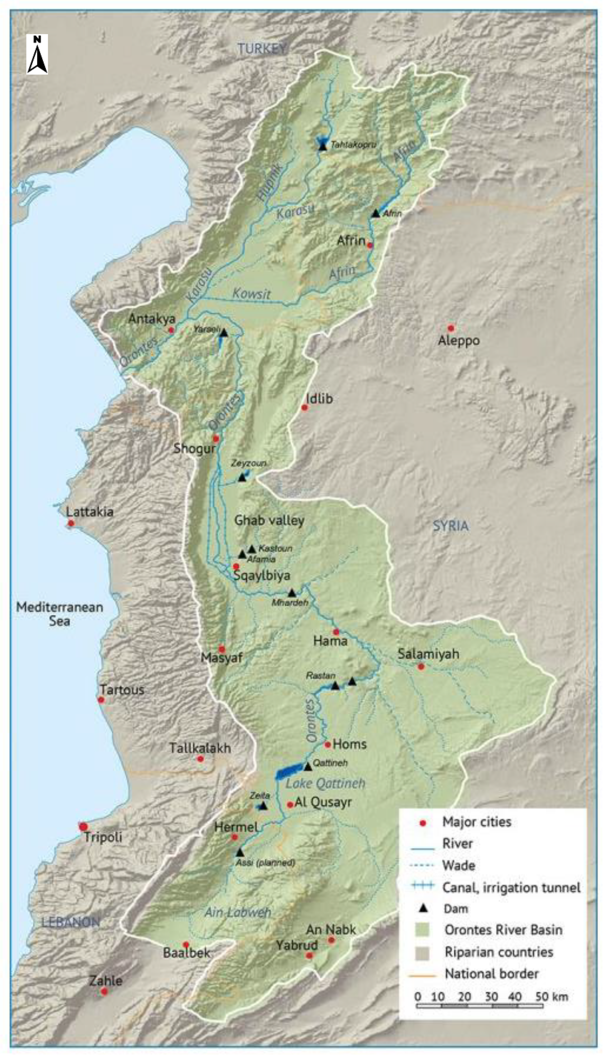
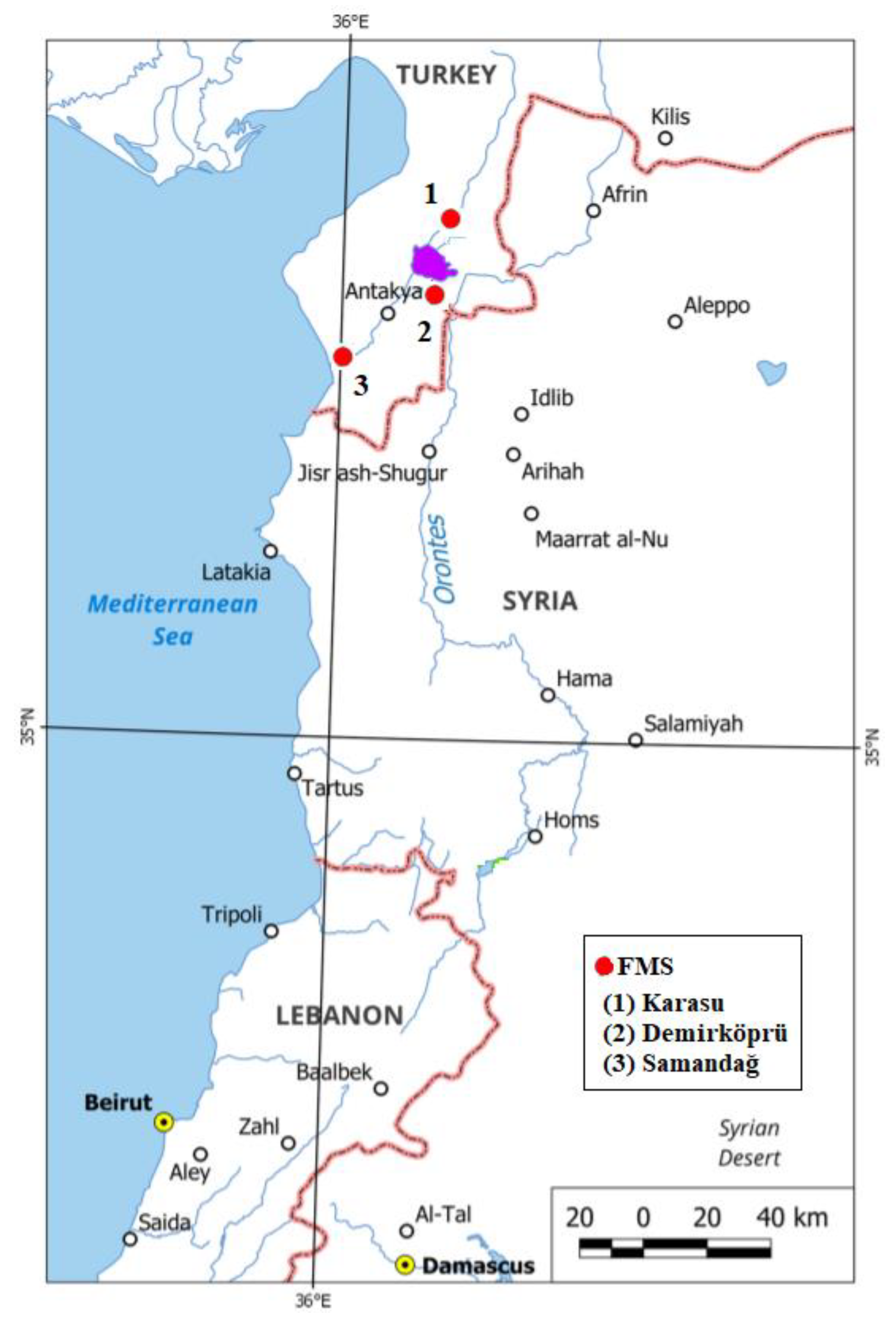
2.1. Study Region

Despite the fact that water scarcity, which is a physical phenomenon, is only a natural phenomenon, it can cause devastating effects due to the vital dependence of society on water resources. In order to minimize the damages of these destructive outcomes, it is necessary for planning to determine the risky regions by using historical hydrological data on a regional basis. The Orontes Basin, located in the south of Turkey and included in the scope of transboundary waters, is essential in terms of the planning of this region due to its geopolitical location. The total water potential for the Orontes basin is determined as 2.64 billion m³/year. Accordingly, 0.27 billion m³/year of water potential derives from Lebanon, about 1.09 billion m³/year from Syria, 0.18 billion m³/year from Afrin, including the waters passing through Syria, and about 1.18 billion m³/year originates from Turkey [34]. It is likewise noteworthy to evaluate the direct current estimations of this basin, of which approximately 55% of the total water potential is from outside our country. The Orontes River, showed in Figure 1, called Asi in Arabic, is located east of the Lebanon Mountains. The river was formed by its slope over some time with the help of Rasel-Ayn and Al-Labwah, which form the main sources. Subsequently, the rivers merge in Syrian territory after crossing the Bekaa valley between the Lebanon and Anti-Lebanon Mountains. Near the humus, it flows by heading first to the northeast and then to the north under the impact of basalt currents. Additionally, the river initiates from the Gharb Plain around Karkur and forms the Turkey–Syria border, starting near the Etun (Zambakiye) village. Near Eşrefli village, it ultimately joins Turkish territory. After proceeding 10 km north on the Amik Plain, the river bends to the southwest by drawing an arc and enters the Mediterranean Sea near Samandağ [35,36].

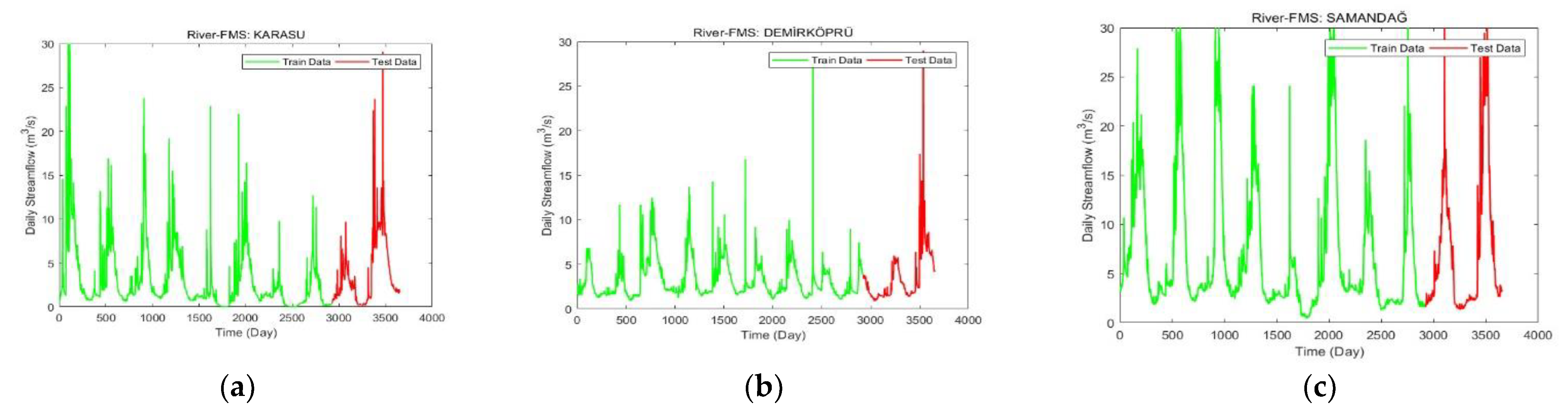
2.2. Datasets and Pre-Processing

In this study, three flow measurement stations that represent various hydrological conditions of the Orontes River Basin were selected to validate the predictive capacity of the generated model. They were chosen in accordance with the conditions of being on various branches of the Orontes River basin shown in Figure 2. Daily flow measurement stations (FMSs) were used to gather long-term, 10-year streamflow data.

Demirköprü FMS (D19A07) is where the Orontes River joins Turkish territory. Karasu FMS (E19A05) is Karasu River, merging with the Orontes River. The Karasu FMS was chosen considering the fact that it passes through the Amik Plain, where intensive agricultural activities take place. Furthermore, the Karasu River merges with the Small Asi River and empties into the sea from Samandağ. Samandağ FMS (D19A09), the point before the Orontes River, spills into the sea. Samandağ station has been determined since it empties into the sea from Samandağ after passing through both the city centers. In addition to that, after merging with the Karasu River, these regions demonstrate intensive agricultural activity. The locations of the stations on the Orontes River are presented with geographical coordinates in

Table 1. General information of FMSs located along the Orontes River.

FMS	River FMS	Coordinates		Cathment Area (km2)	Elevation (m)	Observation(year)
		East	North
		(° ′ ″)	(° ′ ″)
1907	Demirköprü	36 21 28.2	36 14 41	16.170	85	2010–2019
1905	Karasu	36 12 28.3	36 16 41.7	1.768	84	2010–2019
1909	Samandağ	35 59 20.6	36 04 01.9	23.205	11	2009–2018

. As shown in Figure 3, during the observation period, the minimum and maximum rates of flow belonging to the three river stations were 1.78 m³/s and 30 m³/s, respectively.

Taking the streamflow at Demirköprü FMS into account, while the lowest streamflow was 2.09 m³/s in 2017, the highest streamflow was 30 m³/s in 2018. As for the daily streamflow at the Karasu FMS, the lowest streamflow was 1.20 m³/s in 2016, whereas the highest streamflow was 30 m³/s in 2010. In addition, at the Samandağ FMS, the lowest streamflow was observed in 2017 at 1.78 m³/s, and the highest streamflow was found as 29.77 m³/s in 2016. Lastly, the highest streamflow was recorded for three stations in the period of March–May.

In the hybrid model created, Python 3.9, one of the versions of the Python programming language, with new components and optimization, was utilized. In the study, the model benefited from Keras library and Deep library for training processes and prediction processes. In the hybrid model where daily river flow data were analyzed, the LSTM comprised 100 periods for LSTM and eight batch sizes for performance analysis during the training process; while ADAM was the optimizer, MSE was the loss function. The dataset was directly bonded to the flow values for each day, and the flow values were formed by the daily flow, which was taken from EIEI (Electrical Works Survey Administration General Directorate) and DSI (Hydraulic State Works). The original data accumulated from the flow observation stations contained 10 years (3651 days) of operations for each station. Of the total dataset, 80% of the data was obtained as the training set and the remaining 20% as the test set. The data were trained to compare models, and then hybrid model performance was analyzed for test data. In addition, the hybrid model indicated one dense layer and two hidden layers.

In this study, the historical flow data of the stations were analyzed in order to estimate the future river flows and evaluate the proposed models. For this reason, flow data that have not been disrupted in a long time period were included so as to obtain accurate estimation. It is significant that the taken flow data must be recorded completely and not be cut. At this stage, short-term cuts in the flow data are acceptable. However, in many basin-based studies, when meteorological data (precipitation, snow, temperature, evaporation, etc.) and hydrological data (flow observation or flow measurement) are obtained from institutions, the data from past dates might be missing or cut for various reasons, such as climatic difficulties, transportation difficulties, or problems with the measuring device. The formation of gaps in inflow data due to unfavorable climatic conditions or various reasons forms significant issues in terms of effective planning, design, and operation of water resources. In addition, these conditions should be taken into account in determining the flow values so that the structure and hydrological characteristics of the datasets are not deteriorated.

In addition, as stated above, three hydrological stations, Demirköprü, Karasu, and Samandağ, were selected to validate the PSO-LSTM model, which illustrates the various climatic regions and hydrological conditions of the Orontes River. The Orontes River Demirköprü station is located in the Hatay Watershed, one of the basins with a high flood regime. The station is the first measurement station encountered after the Orontes River joins the territory of Turkey. It holds the wide river valley in the upper reaches and is located in the riverbed that extends to the transition zone where the canal turns into a plain. In addition, since the mentioned station is near the borders of Turkey, it is least affected by the interventions to the river waters in Turkey. Karasu Station is located at merging of the Orontes River within the borders of Turkey; it is the last station extension and contains a large part of the catchment area. Samandağ Station maintains the flow of the river to the sea. By use of these features, D19A07, E19A05, and D19A09 stations were utilized to assemble the datasets for this study. The time period of Demirköprü and Karasu stations in the study was between 2010 and 2019. Samandağ station data were from 2009–2018. The datasets consisted of daily flow values.

2.3. Methods

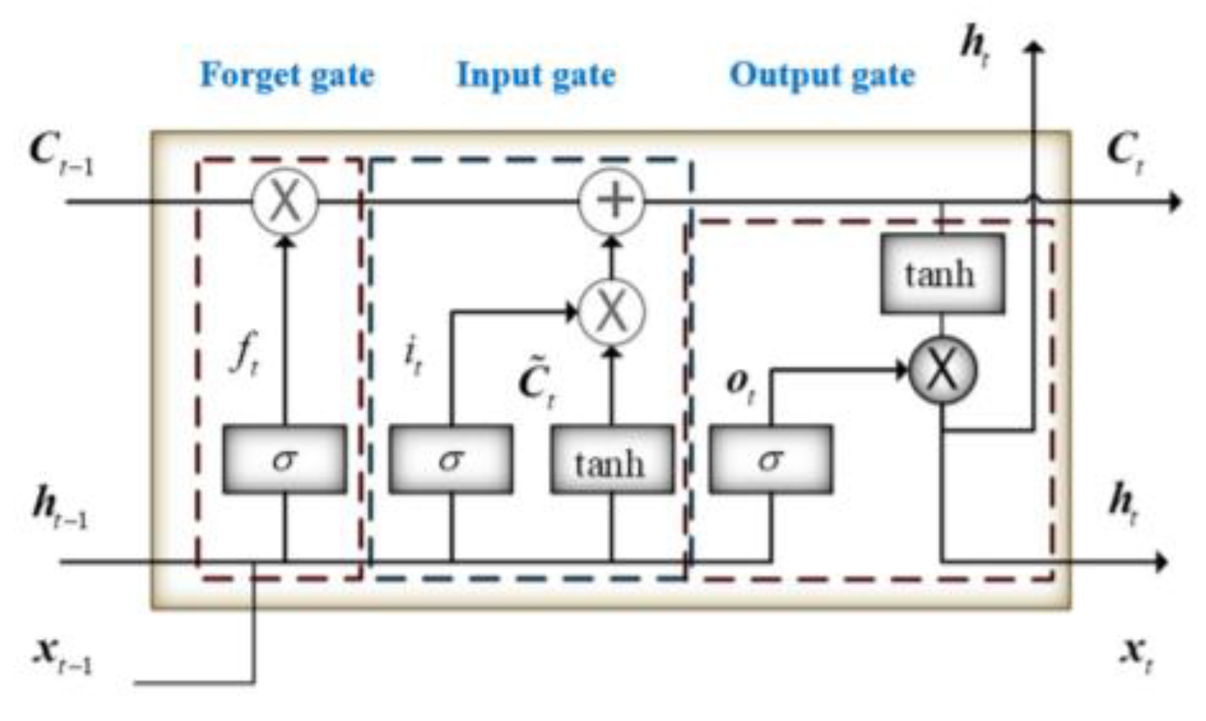
2.3.1. Long Short-Term Memory Network

Long short-term memory (LSTM) is an impressive RNN architecture, and the most noteworthy feature of this advanced architecture is its ability to decode the disappearing gradient situation or at least reduce the impact of the disappearing gradient issues on training performance. Similar to RNN, nodes in an LSTM neural network receive the latent states of the previous step. However, the node, which is a common LSTM unit, contains a more advanced structure than it does in RNN, and this is the primary aspect that provides long-term memory by reducing the vanishing gradient outcome [37]. Three major components create the LSTM’s internal structure—forget undesirable information in the current cell state through the forget gate, add further data to the current cell state through the input gate, produce an output of the current cell state through the output gate—and these serve specific operations on cell states [38]. These gates determine which data need to be added or cleared. Cell State, C_t, can be thought of as the memory of a network. It ensures that previous information is maintained. The gates determine the data to be transported, as shown in Figure 4. In Equation (1), f_t, which is the information from the previous cell, h_t, and the current information, X_t, are inserted into the sigmoid activation function. The forget gate, f_t, determines how much memory is preserved from the previous memory state, C_t−1. Information with 0 is forgotten, and information with 1 continues to be carried by Cell State. Another gate is the input gate, i_t, in Equation (2), providing the information to write into the current memory state, C_t. It updates Cell State, C_t, and decides to update the previous and current information according to the result of the sigmoid (σ) operation. LSTM decides which information it will delete with the sigmoid function. Information with 0 is considered trivial, and information with 1 is deemed essential. In addition, the tanh activation function, which compresses the data between −1 and 1, is used to regulate the network. Then, the sigmoid and tanh function outputs are multiplied, and choose which information will be updated. In Equations (3) and (4), The exit gate determines the input of the next cell, h_{t + 1}. It is also operated for guesswork. Then, the existing information on the Cell State is passed through the tanh function. Finally, it determines what information will be the input for the next cell, h_{t + 1}, by multiplying the two outcomes. When the gate operations for the current cell are completed, the Cell State that will proceed to the next cell and the Hidden State, h_t, information defined as the input information of the cell are decided. In Equations (5) and (6), relying on the current cell state, C_t, the output of LSTM h_t is determined by the output gate o_t [39,40,41].

$$f_t=\sigma \left(W_{f,x}\times X_t+W_{f,h}\times h_{t-1}+b_f\right)$$

(1)

$$i_t=\sigma \left(W_{i,x}\times X_t+W_{i,h}\times h_{t-1}+b_i\right)$$

(2)

$$o_t=\sigma \left(W_{o,x}\times X_t+W_{o,h}\times h_{t-1}+b_o\right)$$

(3)

$${\tilde{C}}_t=\tan h\left(W_{c,x}\times X_t+W_{c,h}\times h_{t-1}+b_c\right)$$

(4)

$$C_t=C_{t-1}\times f_t+i_t\times {\tilde{C}}_t$$

(5)

$$h_t=o_t\times \tan h\left(C_t\right)$$

(6)

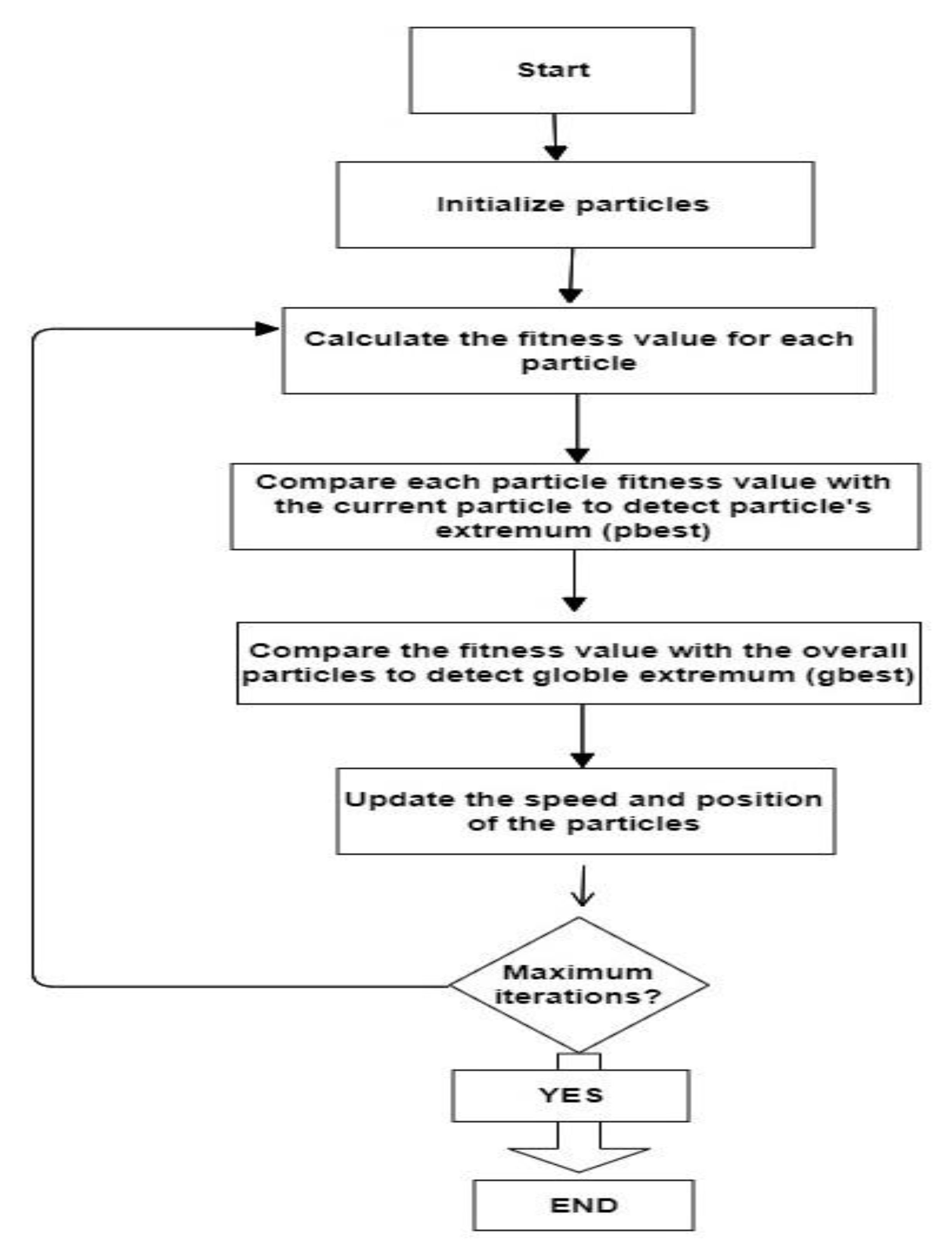
2.3.2. Particle Swarm Optimization

Many global optimization techniques based on a nature-inspired analogy have been generated over several decades. These techniques are beyond the intuition of inhabitants and employ tools that can solve many of the limitations of derivative-based approaches. One of these popular techniques, PSO, developed by Kennedy and Ebert, is a sociologically inspired population-based metaheuristic founded on the simulation of common approaches such as evolutionary programming, ant colony, birds flock, and fish flock. These algorithms have revealed their ability to solve challenging and complex optimization situations in various fields. Compared to the genetic algorithm (GA) and other evolutionary algorithms (EAs), PSO was utilized in this study due to its faster convergence rate and easy implementation [42].

The PSO system is configured with random solutions and searches for the best solution by updating each iteration. Each potential solution, called particle, is represented by a point in the multidimensional solution space. As they are scanning for the optimal solution, the particles pass into the solution space at a certain speed. Each particle adjusts its position and velocity according to its own experience and the experience of its neighbors. Correctly, each particle takes the path of the best solution. This solution is called personal best representative, pbest. The system also preserves the globally optimal path of all swarms, called gbest. The basic concept of PSO involves varying the velocity of each swarm towards the pbest and gbest positions at each repetition [43]. The particle swarm continues iterating through the process illustrated below until an optimal solution is uncovered. The flow chart of the PSO algorithm is depicted in Figure 5.

The PSO system incorporates a local search approach (during self-experimentation) with global approaches (during the adjacent experience) during balancing investigation and exploitation. The state of particles in the study field is explained by particle position, X_i, and particle velocity, V_i.

$$v_i^{\left(t+1\right)}=\omega v_i^t+c_1{r}_1\left(p_i-x_i^t\right)+c_2{r}_2\left(p_g-x_i^t\right)$$

(7)

$$x_i^{\left(t+1\right)}=x_i^t+v_i^{\left(t+1\right)}$$

(8)

The expression V_i = [V_i1, V_i2......V_in] is called the velocity for particle I, which specifies the distance that this particle will travel from its initial position. The expression X_i = [X_i1, X_i2…X_in] specifies the position of particle i. The expression pbest is the previous best position of the thread ‘i’. The expression gbest represents the best position among all herds in the population. The r₁ expression denotes evenly distributed random variables within [0,1]. Expressions C₁ and C₂, called acceleration coefficients, are also greater than 0 and they take each particle to the single best state and optimal particle location, respectively.

The first part of Equation (7), the expression Vi[t], refers to the particle’s previous velocity, which is a memory of the previous extreme direction. This term can be considered the momentum that prevents the particle from altering its direction drastically and that impacts the current direction.

The second part, the expression C₁ × r₁ × (Pbest i[t] − Xi[t]), is called the cognitive part and refers to the particle’s individual experience. This cognitive part resembles the individual memory of the better place for the particle. The consequence of this term is that herds return to their best places, similar to the tendency for individuals to return to the most satisfying situations or places in the past [44,45].

The last part, the expression C₂ × r₂ × (gbest i[t] − Xi[t]), clarifies the association among particles, and it is called the social component. The term is analogous to a group standard that individuals seek to achieve. The outcome of this term is that each particle is attracted to the best position determined by its neighbor. The numbers named r₁ and r₂ are indiscriminate in the range of [0,1].

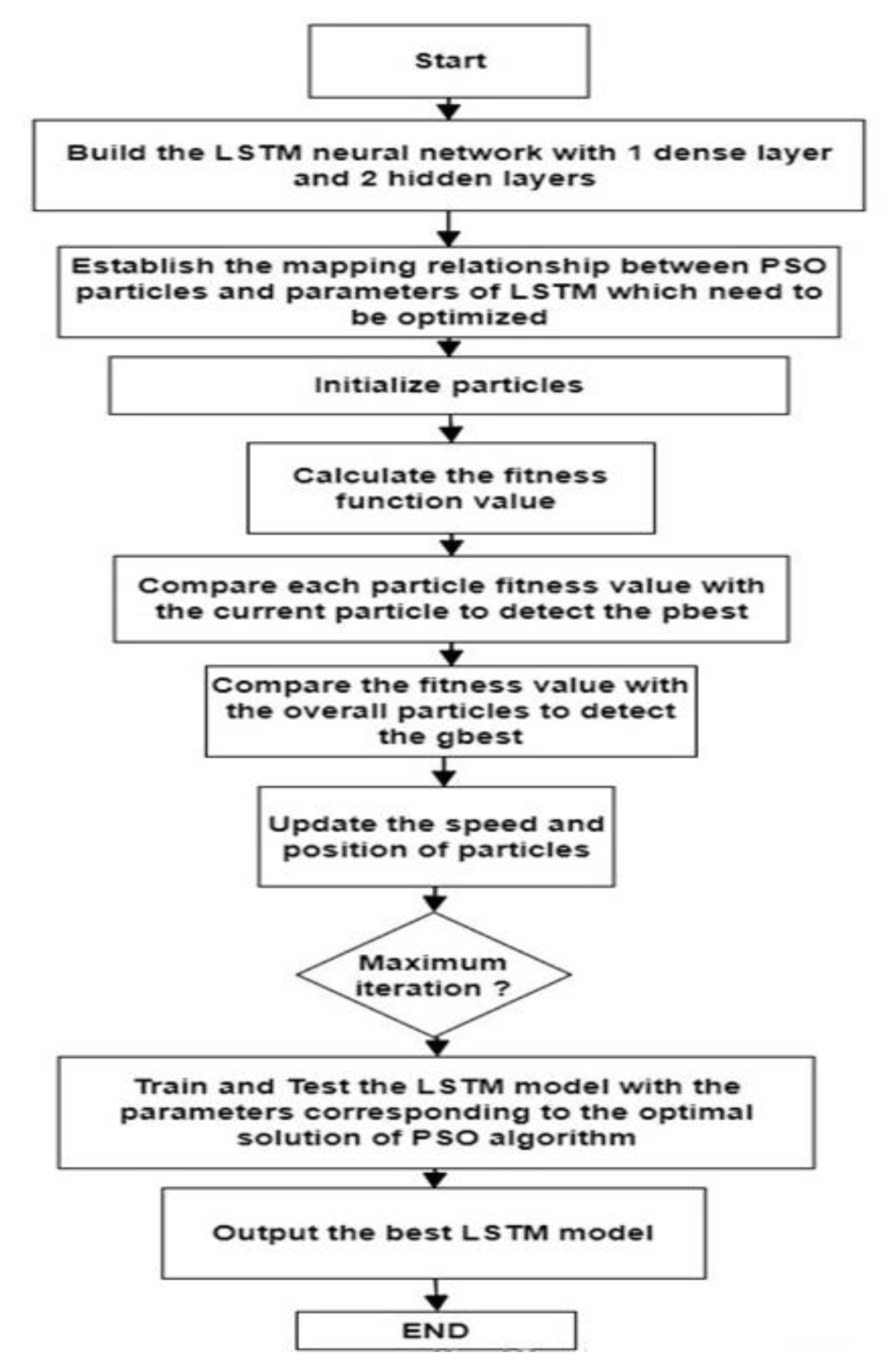
2.3.3. Forecasting Based on PSO-LSTM (Proposed) Model

In the LSTM neural network, the initial values of the parameters critically influence the network’s performance. In this study, the PSO algorithm was employed to optimize two essential parameters of the LSTM network. These two parameters are the number of hidden layer neurons and the learning rate. While constructing the proposed model, a standard LSTM network prediction model was conducted as a priority. The test outcomes were compared by training with random parameters ten times, and the most promising results were documented as the benchmark model. Right after, several hyperparameters of the LSTM model were optimized with PSO. The optimal outcomes of the PSO algorithm were determined, then added to the LSTM network as a parameter, then the LSTM model was retrained, and the outcomes were compared with the benchmark model. In addition, the linear regression model was run to verify the accuracy of the results. Consequently, the results with both models were compared.

First of all, the data were arranged for the training. Therefore, the dataset was divided into training and test datasets by 80% and 20% for the process. Later, translation and normalization techniques were applied so as to optimize the parameters in both datasets. Then, they were converted into a suitable version for training. Afterwards, the LSTM network was first trained with one dense and one LSTM layer. It proceeded as one dense and two LSTM layers to achieve a more pleasing performance. The network structure was accepted as more suitable, and the three-hidden-layer structure was utilized in the following operations. By altering the number of neurons in the hidden layers, the network was run 10 times, and the most acceptable results of the three-layer network were assumed as references. Many attempts were made to determine the most appropriate bias value for the model. As a result of the experiments, the bias value was determined as 0.5. The mapping between PSO particles and LSTM parameters was then merged into this structure. Thus, weight was 0.5, swarm size was 20 and the maximum number of iterations was 50, C₁, and C₂ acceleration constants were in the range of (−2, 2), velocity was in the range (−3, 3), and the number of particles was in the range (32, 256). For the calculation of pbest and gbest values, the results from the PSO were employed as the learning rate. The number of neurons in the proposed network and the R² (coefficient of determination) were used to determine the fitness values. In this paper, r₁ is equal to 0.6, and r₂ is equal to 0.3. The network was utilized with the optimization results corresponding to the gbest, and the results were recorded. After these procedures, the linear regression model was also utilized. The graphs and results of the three models were compared. The flowchart of the hybrid model is shown in Figure 6.

3. Results

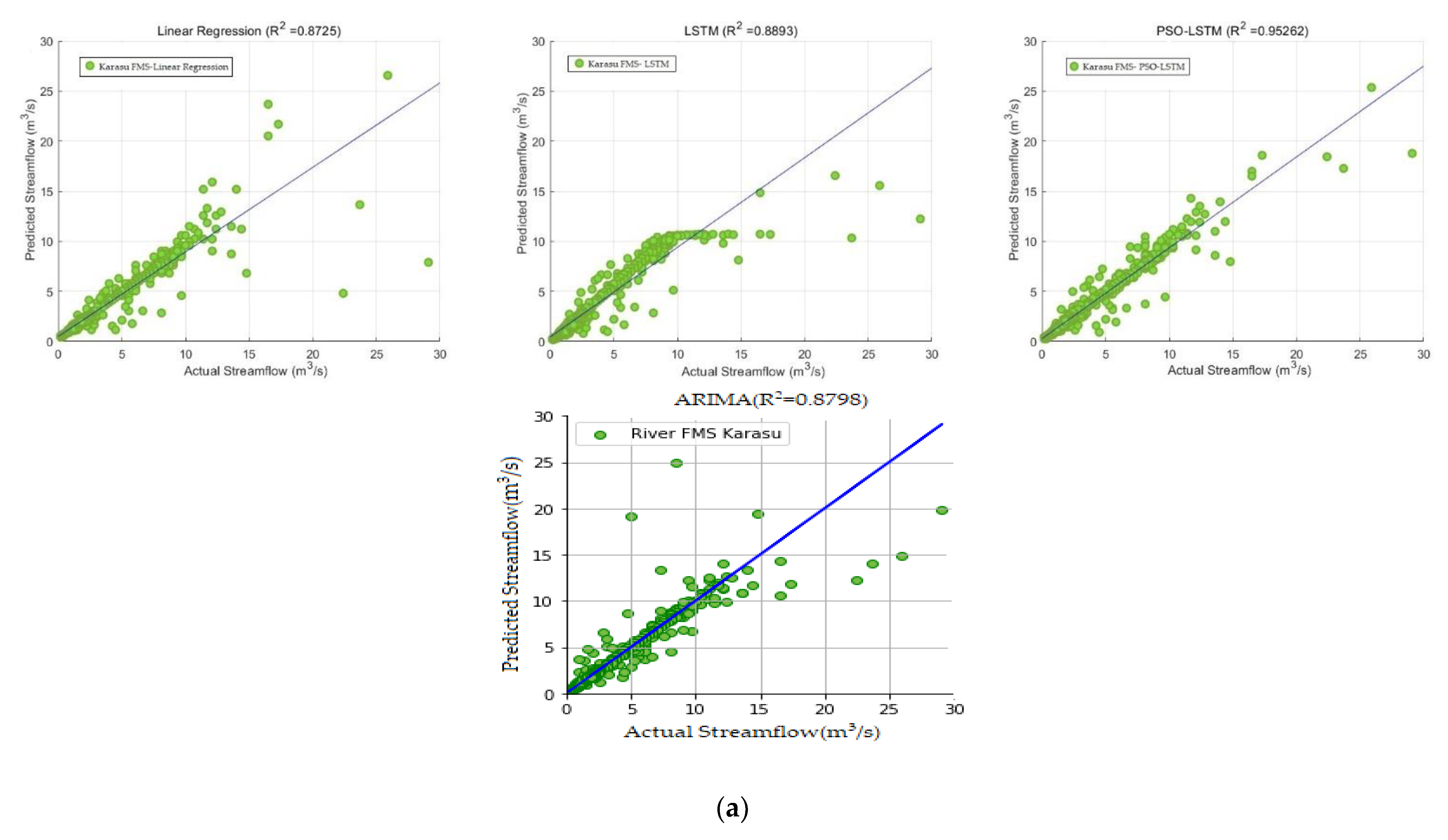
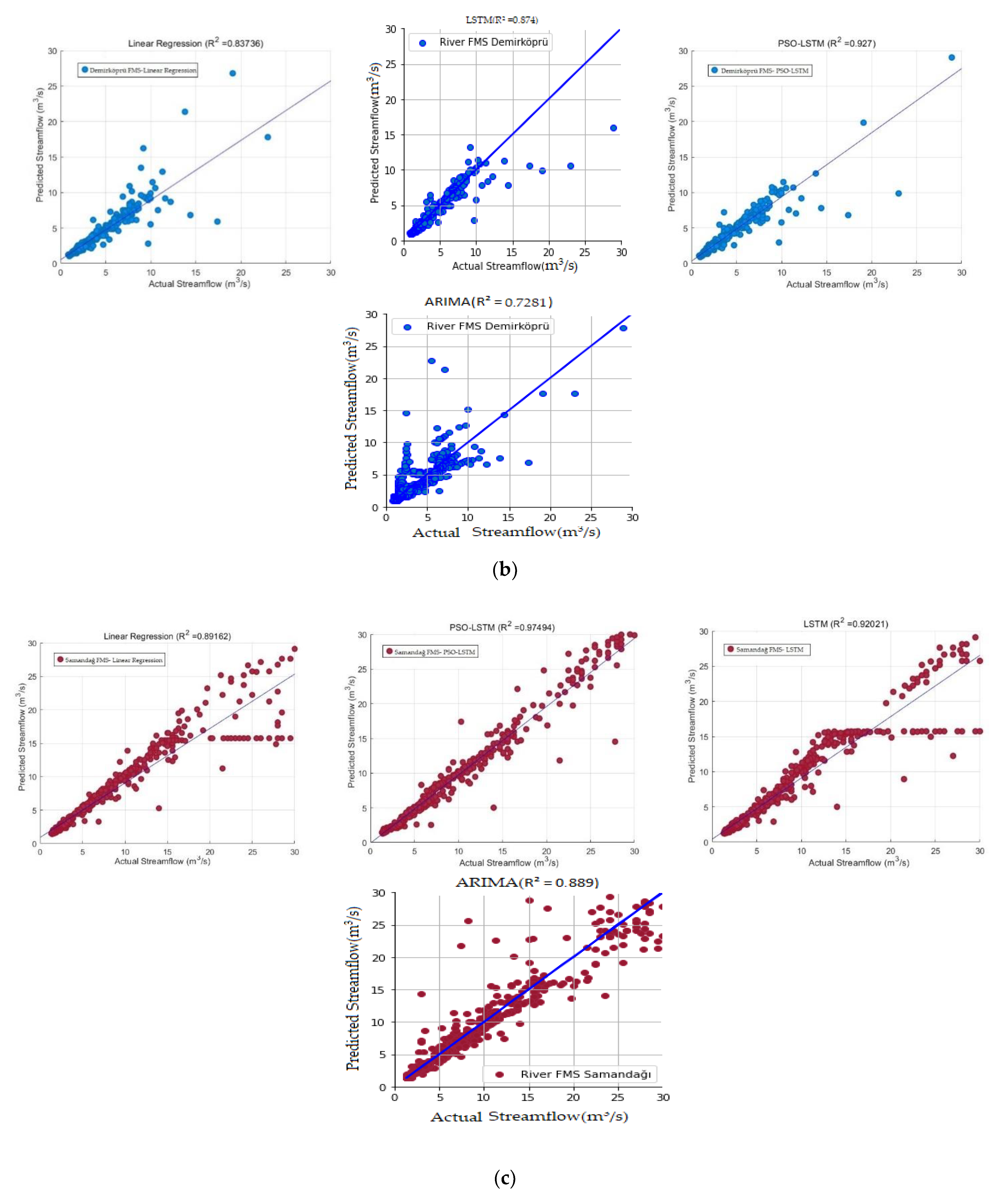
3.1. Performance Evaluation of Models

The hybrid, linear regression and ARIMA models are compared with the benchmark model in this section of the study. One of the well-known and classical linear statistical models for the estimation of time series is the ARIMA model. The ARIMA is a time series estimation approach used to predict the future value of a variable using its past values. The linear regression model was employed to examine the correlation among the data. The linear regression method used the linear function to model the association between dependent and independent variables in the dataset range and tested the linear correlation. Since the regression approach models the dependent variable as a linear function of the independent variables, it provides an interpretable explanation of how the input affects the output [46]. The performance results of each flow measurement station are shown in Figure 7. Five assessment indicators, which were among the common measures of statistical distribution, were employed to study and compare the estimation results. These are RMSE, MAE, MAPE, standard deviation (SD), and R², specified in

Table 2. Forecasting evaluation criteria (all values are in m³/s).

Station	Model	RMSE	MAE	MAPE	SD	R2
Karasu	PSO-LSTM	0.8276	0.1401	14.0196	0.2611	0.9526
	LSTM	1.2363	0.1530	15.3023	0.2942	0.8893
	ARIMA	1.2886	0.0978	9.7838	0.1742	0.8798
	Linear	1.3308	0.1948	19.4855	0.3390	0.8725
	Regression
Demirköprü	PSO-LSTM	0.9073	0.0728	7.2830	0.1545	0.9270
	LSTM	1.2836	0.0714	7.1450	0.1563	0.8740
	ARIMA	1.7860	0.2401	24.0195	0.3006	0.7281
	Linear	1.3498	0.0892	8.9201	0.2129	0.8373
	Regression
Samandağ	PSO-LSTM	1.2557	0.1025	10.2574	0.1541	0.9749
	LSTM	2.3066	0.1270	12.7057	0.1865	0.9202
	ARIMA	2.6255	0.1066	10.6665	0.1647	0.8890
	Linear	2.6876	0.0951	9.5131	0.1902	0.8916
	Regression

. Statistical measurement results of the stations are explained in Table 2. The model’s performance consisted of 730 test data for all three stations. The performance of the hybrid model against other models applied in the study was observed to be thriving when the measurement criteria presented in Table 2 were examined. Furthermore, statistical measurements supported the performance of the hybrid model.

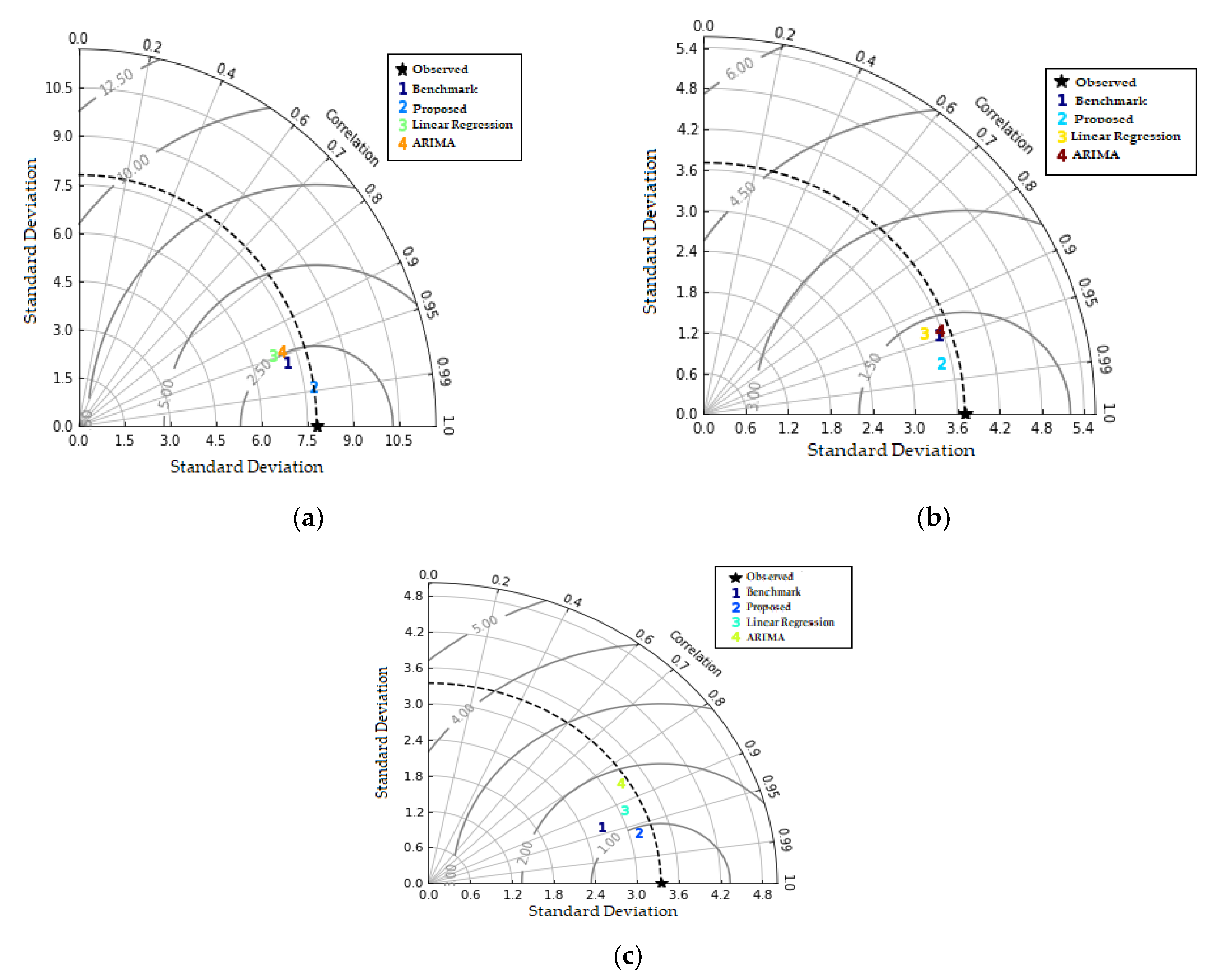
3.2. Comparative Analysis and Discussion

Plotting graphs were used to compare the proposed new PSO-LSTM model. A regression line was also identified in the plotting graphs. The regression line indicated in the graphs was a standard fit line and significant for demonstrating model performance. In this context, while determining the quality of a model, its size and whether it creates a pattern were analyzed. The results of the test data were studied on these graphs. When the plotting graphs of Karasu station, as shown in Figure 7a, are examined, PSO-LSTM presented a very satisfactory performance with 0.95262 R² value compared to LSTM, with 0.8893, ARIMA, with 0.8798, and linear regression, with 0.8725, models. According to the criteria of the R² at Demirköprü station, as shown in Figure 7b, PSO-LSTM outperformed LSTM (0.8740), ARIMA (0.7281), and linear regression (0.8373) models with a value of 0.9270. According to Samandağ station plotting graphs, PSO-LSTM was achieved with an R² value of 0.9749, compared to LSTM with 0.9202, ARIMA with 0.8890, and linear regression 0.8916. The Samandağ station, the last point where the Orontes River empties into the Mediterranean, revealed a strong correlation of the estimated flow data with the daily flow values consistent with its features such as accumulation and acting as a downstream point. Additionally, when the comparison models were examined, it was revealed that the LSTM models were more promising than the linear regression models in all three stations. Analysis of the PSO-LSTM and LSTM methods confirmed the feasibility of the application to flow estimation in the Orontes River basin, with all R² coefficients of PSO-LSTM being greater than (0.92) among three typical hydrological stations. From the analysis of the five evaluation indices, the accuracy of the models was in the order of PSO-LSTM > LSTM > linear regression >ARIMA. It showed that no additional data error was added to the hybrid calculation. On the other hand, the proposed PSO-LSTM hybrid model was reliable and exhibited higher accuracy in daily flow prediction.

Table 2 shows the values of the statistical measurements of the three hydrological stations. At Karasu station, according to the MAE criterion, the LSTM model presented a value of 0.1530 while the hybrid model had a value of 0.1401. The linear regression model showed a value of 0.1948, and the ARIMA model showed a value of 0.0978. When the RMSE criterion was examined, the hybrid, benchmark, linear regression, and ARIMA results were 0.8276, 1.2363, 1.3308, and 1.2886, respectively. According to the standard deviation criterion, these values were similarly 0.2611, 0.2942, 0.3390, and 0.1742. According to the MAPE criterion, these values were 14.0196, 15.3023, 19.4855, and 9.7838. When the evaluation criteria at Karasu station were examined, it was presented that the hybrid model was successful among all evaluation criteria according to the comparison, linear regression, and ARIMA models.

At the Demirköprü station, according to the MAE criteria, the LSTM model had a value of 0.0714, whereas the hybrid model had a value of 0.0728. On the other hand, the linear regression model had a value of 0.0892, and the ARIMA model had a value of 0.2401. When the RMSE criterion was examined, the hybrid, comparison, linear regression, and ARIMA results were 0.9073, 1.2836, 1.3498, and 1.7860, respectively. According to the standard deviation criterion, these values were 0.1545, 0.1563, 0.2129, and 0.3006, respectively. According to the MAPE criterion, these values were 7.2830, 7.1450, 8.9201, and 24.0195. When the evaluation criteria at Demirköprü station were analyzed, it was detected that the comparison model was successful, despite a slight difference in the MAPE and MAE evaluation criteria. Likewise, it was quite successful compared to the linear regression. In the other three statistical measurements, the hybrid model was successful compared to the comparison, linear regression, and ARIMA models.

At the last station, Samandağ, according to the MAE criterion, the LSTM model had a value of 0.1270 while the hybrid model had a value of 0.1025. On the other hand, the linear regression model had a value of 0.0951, and the ARIMA model had a value of 0.1066. When the RMSE criterion was investigated, the results of hybrid, comparison, linear regression, and ARIMA models were 1.2557, 2.3066, 2.6876, and 2.6255, respectively. According to the standard deviation criterion, these values were −0.1541, 0.1865, 0.1902, and 0.1647, respectively. According to the MAPE criterion, these values were 10.2574, 12.7057, 9.5131, and 10.6665. When the evaluation criteria at the Demirköprü station were examined, the hybrid and linear regression models provided similar results according to the MAPE and MAE evaluation criteria. The benchmark model lagged behind the hybrid and linear regression models in these criteria. In other evaluation criteria, the hybrid model was quite successful compared to the benchmark and linear regression models. At the Demirköprü station, the ARIMA model lagged behind other models in all evaluation criteria.

In addition, when all evaluation criteria for the three stations were examined, the hybrid model provided significant improvements in percentage. In the general evaluation, the values with the highest R² and the lowest standard deviation were seen at the Samandağ station. Demirköprü station came to the fore in MAE and MAPE evaluations, and Karasu station according to RMSE criteria. As mentioned before, the Karasu station is located where the Orontes River merges, the river spills into the sea over the last point, Samandağ, and the region where Demirköprü station is located is not exposed to pollutants originating from Turkey when the Orontes River enters the borders of Turkey, and the precipitation area capacities of the three stations reveal differences when compared with each other.

Streamflow in Karasu was generally in the range of 0–15 m³/s, and the best estimates were in the range of 0–10 m³/s for all methods. Actual measurements in the range of 10–15 m³/s reach 10 m³/s according to the LSTM results. For other models, the prediction success in this value range was similar; the method to produce results closest to the actual values was PSO-LSTM. For the streamflow in the range of 15–30 m³/s, which includes the highest and outliers, the estimation values of LSTM did not exceed 18 m³/s. While linear regression predicted flows in the 15–20 m³/s range, the results were above the real values and below the actual values in ARIMA. At this point, the PSO-LSTM hybrid model exhibited its success and made accurate predictions in the 15–20 m³/s range. For values above 20 m³/s, the hybrid model is in the closest value range to the trend line, and its success at this point has greatly contributed to its superiority over other models.

Demirköprü measured current values showed intensity between 2–10 m³/s. In spite of the fact that the estimated values were concentrated in this range, the ARIMA values currents in the 2–3 m³/s value range to those in the 5–10 m³/s value range, and it distributed the currents in the 5–10 m³/s value range to the 5–25 m³/s value range. It caused the accuracy of the model to be low among other models. Other models made predictions in the same range for the measured values between 0 and 12 m³/s. Current values above 14 m³/s greatly influenced the success of the models. Likewise, the model with the least deviations and errors was the hybrid model.

Samandağı current measurement values have the widest range. The striking point here is that LSTM and linear regression models tend to cluster in the same value range, the 12–30 m³/s value range. Although ARIMA generally moves in the direction of the trend line, the hybrid model gave much more accurate results as the intervals are far from the hybrid model.

Figure 8 illustrates the standard deviation (SD) and correlation for benchmark (1), proposed (2), linear regression (3), and ARIMA (4) models in Taylor diagram. The distance from reference to the point (observed) measures the centered RMSE [47]. Thus, the reference point with the correlation coefficient marks a perfect model equal to 1 (existence in full agreement with the observations) and the same amplitude of variation when compared with the observations [48]. At all three stations, the hybrid model results were closer to the observation points compared to the other model results, confirming the better accuracy of the optimized model. In spite the fact that the benchmark model performed more sufficiently at Samandağ and Demirköprü stations than ARIMA and linear regression did, the ARIMA model provided a significantly close results to the benchmark model at Karasu station, but lagged behind linear regression.

To show that the hybrid model used in this study has high accuracy in forecasting river flows, we compared the estimation results of the literature using hybrid models to predict time series.

Jabbari and Bae [49] evaluated the real-time bias correction of precipitation data, and from a hydrometeorological point of view, an assessment of hydrological model improvements in real-time flood forecasting for the Imjin River (South and North Korea) was performed. The performance of the real-time flood forecast improved using the ANN bias correction method. Jiandong et al. [50] developed a hybrid forecasting model. In the study, the long short-term memory neural networks (LSTMs) and deep belief networks based on particle swarm optimization (PSO-DBN) were utilized to construct sub-series prediction models. The results showed that the proposed method in this paper was more effective than the other existing methods were. Wang et al. [51] proposed a hybrid model-based “feature decomposition-component prediction-result reconstruction” named VMD-LSTM-PSO to cope with the nonlinear and nonstationary challenges that conventional runoff forecasting models face and improve daily runoff prediction accuracy. Based on its high predictive accuracy and stability, the novel model promised to be a preferred data-driven tool for hydrological forecasting in practice. Chen et al. [52] utilized the three popular DL models, which were deep neural network (DNN), temporal convolution neural network (TCN), and long short-term memory neural network (LSTM). They were used to estimate daily reference evapotranspiration (ETₒ). The results displayed that all proposed DL and CML models outperformed radiation-based or humidity-based empirical equations beyond the study areas in which they were trained. Di Nunno et al. [53] predicted spring flows by applying nonlinear autoregressive with exogenous inputs (NARX) neural networks. The good results achieved recommend using the NARX network for spring discharge prediction in other areas characterized by karst aquifers. Granata and Di Nunno [54] built three recurrent neural network-based models to predict short-term actual evapotranspiration. Two variants of each model were developed, changing the employed algorithm, selecting between long short-term memory (LSTM) and nonlinear autoregressive network with exogenous inputs (NARX). The results revealed that deep learning-based models could provide very accurate predictions of actual evapotranspiration; however, the performance of the models can be significantly impacted by local climatic circumstances. As can be seen, the results obtained in many studies show that hybrid models created with PSO outperform the comparative model and provide estimation precision.

Considering all these details, it was noticed that converting the results from the PSO algorithm to LSTM parameters was critical. PSO has several limitations such as stability, patterns of movements, convergence to a local optimum, and expected first hitting [55]. According to known features of PSO, it was thought that it would be correct to integrate it into the model. The PSO algorithm was utilized to optimize the learning rate and the number of hidden neurons, which were two essential parameters of the LSTM network. As a result, it was seen that the improvement rates were quite high. However, the LSTM neural network is complex and has other parameters affecting the prediction performance. The models that will be formed by determining the parameters such as dropout, number of iterations, and batch size other than just the two considered parameters with PSO, or those that integrate the parameters into the proposed model using a different improvement algorithm will guide future studies. In addition, it is thought that the study can be a reference to hybrid methods in the development of methods that are diversifying with each passing day with deep learning techniques and in the search for more suitable parameters in these complex structures.

The hybrid model successfully estimated the daily flow rate in flow measurement station data of three various hydrological conditions. In addition, the study demonstrated the success of the hybrid model in predicting the optimal level of river flows when compared with the benchmark and linear regression models.

To sum up, it can be seen from the results (Table 2 and Figure 6) that of the three overall datasets, the PSO-LSTM achieved the best performance on three of the five evaluation criteria. The estimation results of the PSO-LSTM were superior to those of the LSTM and linear regression models in nearly all cases, except for the last two statistical measurement methods, MAE and MAPE, for river flow datasets. In conclusion, the estimation results indicated that the proposed PSO-LSTM algorithm achieves the best overall results compared with the LSTM model and the regression model for river flow estimation issues.

4. Conclusions

In this study, a hybrid method in which PSO is integrated into LSTM is proposed to estimate flow data. The performance of the proposed method has been tested on river flow data from three different flow observation stations on the Orontes River. In spite of the fact that it has been revealed in the studies that flow can be predicted successfully with artificial neural network, which provides better results than does regression analysis, the success of the method depends on the availability of healthy, reliable, and sufficient data. The proposed new hybrid model was compared with the benchmark model and the linear regression model. Even though the basic LSTM generally demonstrates a strong learning ability for time series, it can occasionally present poor performance results owing to the random selection of initialization parameters. In these cases, supporting the model with optimization algorithms influences the performance considerably. In this study, one of the reasons for choosing PSO as the optimization algorithm to search for the appropriate values of the LSTM parameters is that, when compared to genetic algorithms, it performs with real numbers and has some benefits such as not needing binary coding to make calculations. Statistical evaluation criteria, which are among the basic statistical evaluation methods, were used to measure the model’s performance [56]. The results obtained show that in the proposed PSO-LSTM approach, the estimation errors of the flow data are quite low compared to the other models used in the study. Furthermore, when the R² values are considered, it is seen that the estimation accuracy is quite high for the proposed model at the same rate, which shows that the improvement effect is significant. In addition, the parameters of the PSO algorithm used in this study are among some of the factors that need to be developed for future studies. For this reason, in new hybrid models to be made with the PSO algorithm, a new algorithm will be presented by studying the factors that will affect the model, such as particle number, particle size, particle spacing, learning factors, stopping condition, rate of change, particle swarm size, speed, and the maximum number of iterations. Combining the PSO algorithm with different optimization methods and comparing the PSO algorithm with new algorithms will benefit future research. In addition, new hybrid models to be created using metaheuristic techniques will also be beneficial in future studies. It has been seen that the PSO-LSTM model provides promising results in river flow predictions. However, the study has some limitations. In this study, only flow data were operated as input. Flow time series are nonlinear, and many parameters such as humidity, snowmelt, and temperature can form these time series. This study can be reconstructed with different input parameters and prepare the ground for future studies. Since the data are nonlinear, decomposition techniques can be included in the model. The generated hybrid model was evaluated only for daily flow data. It can be evaluated for shorter time intervals (hourly, 30 min, 15 min) in possible future studies. Other hydrological variables can be applied in the field of hydrology to study of the proposed model. The contribution of the PSO algorithm to the model designed when hybridized is promising. However, the comparison model can be hybridized with other recently popular algorithms (e.g., grey wolf algorithm), and the contribution of the two algorithms to the prediction accuracy can be examined.

References

1. Cosgrove, W.J.; Loucks, D.P. Water management: Current and future challenges and research directions. Water Resour. Res. 2015, 51, 4823–4839. [Google Scholar] [CrossRef] [Green Version]
2. Özcan, T.İ.A. Multiple Reservoir Operation Applications in Water Resources Management. Master’s Thesis, Istanbul Technical University, Istanbul, Turkey, 2021. [Google Scholar]
3. Dalkiliç, H.Y.; Hashimi, S.A. Prediction of daily streamflow by using artificial neural networks (ANNs), wavelet neural networks (WNNs), and adaptive neuro-fuzzy inference system (ANFIS) models. Water Supply 2020, 20, 1396–1408. [Google Scholar] [CrossRef] [Green Version]
4. Xie, T.; Zhang, G.; Hou, J.; Xie, J.; Lv, M.; Liu, F. Hybrid Forecasting Model for Non-stationary Daily Runoff Series: A Case Study in the Han River Basin, China. J. Hydrol. 2019, 577, 123915. [Google Scholar] [CrossRef]
5. Zhu, S.; Zhou, J.; Ye, L. Streamflow estimation by support vector machine coupled with different methods of time series decomposition in the upper reaches of Yangtze River, China. Environ. Earth Sci. 2016, 75, 531. [Google Scholar] [CrossRef]
6. Xu, Z.; Zhou, J.; Mo, L.; Jia, B.; Yang, Y.; Fang, W.; Qin, Z. A Novel Runoff Forecasting Model Based on the Decomposition-Integration Prediction Framework. Water 2021, 13, 3390. [Google Scholar] [CrossRef]
7. Sharma, P.J.; Patel, P.L.; Jothiprakash, V. Data-driven modelling framework for streamflow prediction in a physio-climatically heterogeneous river basin. Soft Comput. 2021, 25, 5951–5978. [Google Scholar]
8. Shortridge, J.E.; Guikema, S.D.; Zaitchik, B.F. Machine learning methods for empirical streamflow simulation: A comparison of model accuracy, interpretability, and uncertainty in seasonal watersheds. Hydrol. Earth Syst. 2016, 20, 2611–2628. [Google Scholar] [CrossRef] [Green Version]
9. He, X.; Luo, J.; Li, P.; Zuo, G.; Xie, J. A Hybrid Model Based on Variational Mode Decomposition and Gradient Boosting Regression Tree for Monthly Runoff Forecasting. Water Resour. Manag. 2020, 34, 865–884. [Google Scholar] [CrossRef]
10. Yaseen, Z.M.; Kisi, O.; Demir, V. Enhancing long-term streamflow forecasting and predicting using periodicity data component: Application of artificial intelligence. Water Resour. Manag. 2016, 30, 4125–4151. [Google Scholar]
11. Nourani, V. Davanlou.; Tajbakhsh, A.; Molajou, A.; Gokcekus, H. Hybrid wavelet-M5 model tree for rainfall-runoff modeling. J. Hydrol. Eng. 2019, 24, 90–102. [Google Scholar] [CrossRef]
12. Mehdizadeh, S.; Fathian, F.; Adamowski, J.F. Hybrid artificial intelligence-time series models for monthly streamflow modeling. Appl. Soft Comput. 2019, 80, 873–887. [Google Scholar] [CrossRef]
13. Arab, M.; Faramarz, M.G.; Hashim, K. Applications of Computational and Statistical Models for Optimizing the Electrochemical Removal of Cephalexin Antibiotic from Water. Water 2022, 14, 344. [Google Scholar] [CrossRef]
14. Sutskever, I.; Vinyals, O.; Le, Q.V. Sequence to sequence learning with neural networks. In Proceedings of the Advances in Neural Information Processing Systems 27: Annual Conference on Neural Information Processing Systems 2014, Montreal, QC, Canada, 8–13 December 2014; Volume 27, pp. 3104–3112. [Google Scholar]
15. Kisi, O.; Choubin, B.; Deo, R.C.; Yaseen, Z.M. Incorporating synoptic-scale climate signals for streamflow modelling over the Mediterranean region using machine learning models. Hydrol. Sci. J. 2019, 64, 1240–1252. [Google Scholar] [CrossRef]
16. Lin, S.S.; Zhang, N.; Zhou, A.; Shen, S.L. Time-series prediction of shield movement performance during tunneling based on hybrid model. Tunn. Und. Spc. Technol. 2022, 119, 104245. [Google Scholar] [CrossRef]
17. Albo-Salih, H.; Mays, L.W.; Che, D. Application of an Optimization/Simulation Model for the Real-Time Flood Operation of River-Reservoir Systems with One and Two-Dimensional Unsteady Flow Modeling. Water 2022, 14, 87. [Google Scholar] [CrossRef]
18. Raghuwanshi, N.S.; Singh, R.; Reddy, L.S. Runoff and sediment yield modeling using artificial neural networks: Upper Siwane River, India. J. Hydrol. Eng. 2006, 11, 71–79. [Google Scholar] [CrossRef]
19. Santra, A.S.; Lin, J.-L. Integrating Long Short-Term Memory and Genetic Algorithm for Short-Term Load Forecasting. Energies 2019, 12, 2040. [Google Scholar] [CrossRef] [Green Version]
20. Duc, H.N.; Le, X.H.; Heo, J.-Y.; Bae, D.-H. Development of an Extreme Gradient Boosting Model Integrated with Evolutionary Algorithms for Hourly Water Level Prediction. Access IEEE 2021, 9, 125853–125867. [Google Scholar]
21. Yan, J.; Chen, X.; Yu, Y.; Zhang, X. Application of a Parallel Particle Swarm Optimization-Long Short-Term Memory Model to Improve Water Quality Data. Water 2019, 11, 1317. [Google Scholar] [CrossRef] [Green Version]
22. Mohammadi, B.; Guan, Y.; Moazenzadeh, R.; Safari, M.J.S. Implementation of hybrid particle swarm optimization-differential evolution algorithms coupled with multi-layer perceptron for suspended sediment load estimation. Catena 2020, 10, 105024. [Google Scholar] [CrossRef]
23. Gharabaghi, B.; Bonakdari, H.; Ebtehaj, I. Hybrid evolutionary algorithm based on PSOGA for ANFIS designing in prediction of no-deposition bed load sediment transport in sewer pipe. In Intelligent Computing, Proceedings of the 2018 Computing Conference, London, UK, 10–12 July 2018; Springer: Cham, Switzerland, 2018; Volume 2, pp. 106–118. [Google Scholar]
24. Meshram, S.G.; Ghorbani, M.A.; Deo, R.C.; Kashani, M.H.; Meshram, C.; Karimi, V. New approach for sediment yield forecasting with a two-phase feedforward neuron network-particle swarm optimization model integrated with the gravitational search algorithm. Water Resour. Manag. 2019, 33, 2335–2356. [Google Scholar] [CrossRef]
25. Motahari, M.; Mazandaranizadeh, H. Development of a PSO-ANN Model for Rainfall-Runoff Response in Basins, Case Study: Karaj Basin. Civ. Eng. J. 2017, 3, 35–44. [Google Scholar] [CrossRef]
26. Zounemat-Kermani, M.; Mahdavi-Meymand, A.; Fadaee, M.; Batelaan, O.; Hinkelmann, R. Groundwater quality modeling: On the analogy between integrative PSO and MRFO mathematical and machine learning models. Environ. Qual. Manag. 2021, 1–11. [Google Scholar] [CrossRef]
27. Xinqing, Y.; Yuan, C.; Yang, Y.; Xuemei, L. Monthly runoff prediction using modified CEEMD-based weighted integrated model. J. Water Clim. Change 2021, 5, 1744–1760. [Google Scholar]
28. Asadnia, M.; Chua, L.H.C.; Qin, X.S.; Asce, A.M.; Talei, A. Improved Particle Swarm Optimization–Based Artificial Neural Network for Rainfall-Runoff Modeling. J. Hydrol. Eng. 2014, 19, 1320–1329. [Google Scholar] [CrossRef]
29. Dökme, F.S. Application of Particle Swarm Optimization for Computer Aided Diagnosis of Diseases. Master’s Thesis, Çukurova University, Adana, Turkey, 2019. [Google Scholar]
30. Feng, R.; Fan, G.; Lin, J.; Yao, B.; Guo, Q. Enhanced long short-term memory model for runoff prediction. J. Hydrol. Eng. 2021, 26, 4020063. [Google Scholar] [CrossRef]
31. Adnan, M.R.; Mostafa, R.R.; Kisi, O.; Yaseen, Z.M.; Shahid, S.; Kermani, Z.M. Improving streamflow prediction using a new hybrid ELM model combined with hybrid particle swarm optimization and grey wolf optimization. Knowl. Based Syst. 2021, 231, 107379. [Google Scholar] [CrossRef]
32. Kuok, K.K.; Harun, S.; Shamsuddin, S.M. Particle swarm optimization feedforward neural network for modelling runoff. Int. J. Environ. Sci. Technol. 2010, 7, 67–78. [Google Scholar] [CrossRef] [Green Version]
33. Sihag, P.; Esmaeilbeiki, F.; Singh, B.; Ebtehaj, I.; Bonakdari, H. Modeling unsaturated hydraulic conductivity by hybrid soft computing techniques. Soft Comput. 2019, 23, 12897–12910. [Google Scholar] [CrossRef]
34. Gumus, V. Hydrological Drought Analysis of Asi River Basin with Streamflow Drought Index. GU J. Sci. Part C 2017, 5, 65–73. [Google Scholar]
35. Tomilova, A.A.; Lyubas., A.A.; Kondakov, A.V.; Konopleva, E.S.; Vikhrev, I.V.; Gofarov, M.Y.; Bolotov, I.N. An endemic freshwater mussel species from the Orontes River basin in Turkey and Syria represents duck mussel’s intraspecific lineage: Implications for conservation. Limnologica 2020, 84, 125811. [Google Scholar] [CrossRef]
36. Korkmaz, H.; Karataş, A. Water management on the Asi (Orontes) River and appeared problems. Mustafa Kemal Univ. J. Soc. Sci. Inst. 2009, 12, 18–40. [Google Scholar]
37. Şırlancı, M. Malicious Code Detection: Run Trace Analysis by LSTM. Master’s Thesis, Middle East Technical University, Ankara, Turkey, 2021. [Google Scholar]
38. Holland, J.H. Adaptation in Natural and Artificial Systems; University of Michigan Press: Ann Arbor, MI, USA, 1975; p. 183. [Google Scholar]
39. Chollet, A. Deep Learning with Pyhton, 1st ed.; Manning Publications: Shelter Islands, NY, USA, 2018; pp. 198–202. [Google Scholar]
40. Liu, L.; Zou, S.; Yao, Y.; Wang, Z. Forecasting Global Ionospheric TEC Using Deep Learning Approach. Space Weather 2020, 18, e2020SW002501. [Google Scholar] [CrossRef]
41. Yıldız, I. Forecasting of Global Vertical Total Electron Content Based on Trigonometric B-Spline with Long Short-Term Memory. Master’s Thesis, Hacettepe University, Ankara, Turkey, 2021. [Google Scholar]
42. Kennedy, J.; Eberhart, R.C. A Discrete Binary Version of the Particle Swarm Algorithm. In Proceedings of the 1997 IEEE International Conference on Systems, Man, and Cybernetics. Computational Cybernetics and Simulation, Orlando, FL, USA, 12–15 October 1997. [Google Scholar]
43. Medina, A.J.R.; Pulido, G.T.; Torres, J.G.R. A Comparative Study of Neighborhood Topologies for Particle Swarm Optimizers. In Proceedings of the International Joint Conference on Computational Intelligence, Funchal, Portugal, 5–7 October 2009. [Google Scholar]
44. Khalaf, T.Z. Hybrid PSO-ANN and PSO Models Based Approach for Estimation of Costs and Duration of Construction Projects. Master’s Thesis, Kastamonu University, Kastamonu, Turkey, 2020. [Google Scholar]
45. Tunchan, C. Particle Swarm Optimization Approach to Portfolio Optimization. Nonlinear Anal. Real World 2009, 10, 2396–2406. [Google Scholar]
46. He, Q.Q.; Wu, C.; Si, Y.W. LSTM with particle Swam optimization for sales forecasting. Elect. Comm. Res. 2022, 51, 101118. [Google Scholar] [CrossRef]
47. Taylor, K.E. Summarizing multiple aspects of model performance in a single diagram. J. Geophys Res. 2001, 106, 7183–7192. [Google Scholar] [CrossRef]
48. Heo, K.Y.; Ha, K.J.; Yun, K.S.; Lee, S.S.; Kim, H.J.; Wang, B. Methods for uncertainty assessment of climate models and model predictions over East Asia. Int. J. Climatol. 2014, 34, 377–390. [Google Scholar] [CrossRef]
49. Jabbari, A.; Bae, D.-H. Application of Artificial Neural Networks for Accuracy Enhancements of Real-Time Flood Forecasting in the Imjin Basin. Water 2018, 10, 1626. [Google Scholar] [CrossRef] [Green Version]
50. Duan, J.; Wang, P.; Ma, W.; Fang, S.; Hou, Z. A novel hybrid model based on nonlinear weighted combination for short-term wind power forecasting. Int. J. Electr. Power Energy Syst. 2022, 134, 107452. [Google Scholar] [CrossRef]
51. Wang, Z.Y.; Qiu, J.; Li, F.F. Hybrid Models Combining EMD/EEMD and ARIMA for Long-Term Streamflow Forecasting. Water 2018, 10, 853. [Google Scholar] [CrossRef] [Green Version]
52. Chen, Z.; Zhu, Z.; Jiang, H.; Sun, S. Estimating Daily Reference Evapotranspiration Based on Limited Meteorological Data Using Deep Learning and Classical Machine Learning Methods. J. Hydrol. 2020, 591, 125286. [Google Scholar] [CrossRef]
53. Di Nunno, F.; Granata, F.; Gargano, R.; de Marinis, G. Prediction of spring flows using nonlinear autoregressive exogenous (NARX) neural network models. Environ. Monit Assess. 2021, 193, 350. [Google Scholar] [CrossRef]
54. Granata, F.; Di Nunno, F. Fabio. Forecasting evapotranspiration in different climates using ensembles of recurrent neural networks. Agric. Water Manag. 2021, 255, 107040. [Google Scholar] [CrossRef]
55. Bonyadi, M.R.; Michalewicz, Z. Particle swarm optimization for single objective continuous space problems: A review. Evol. Comput. 2016, 8, 1–54. [Google Scholar] [CrossRef] [PubMed]
56. Kilinc, H.C.; Haznedar, B. A Hybrid Model for Streamflow Forecasting in the Basin of Euphrates. Water 2022, 14, 80. [Google Scholar] [CrossRef]
Figure 1. Location and topography of the lower Orontes River basin.
Water 14 00490 g001
Figure 2. Study sites in the Orontes River basin.
Water 14 00490 g002
Figure 3. Training (green) and test data (red) of daily streamflow for (a) Karasu, (b) Demirköprü, and (c) Samandağ stations.
Water 14 00490 g003
Figure 4. The interior design of an LSTM cell.
Water 14 00490 g004
Figure 5. Flow chart of PSO algorithm.
Water 14 00490 g005
Figure 6. Flow chart of the PSO-LSTM model.
Water 14 00490 g006
Figure 7. Karasu (a), Demirköprü (b), and Samandağ (c) FMSs model results.
Water 14 00490 g007aWater 14 00490 g007b
Figure 8. Predicted streamflow of the Samandağ (a), Karasu (b), and Demirköprü (c) FMSs in testing period (Taylor diagram).
Water 14 00490 g008