
Impacts of Climate Alteration on the Hydrology of the Yarra River Catchment, Australia Using GCMs and SWAT Model

 ,
,  ,
,  ,
,  ,
,  and
and 
Abstract
:1. Introduction
- To assess the potential effects of future climate alteration on the hydrology of the middle Yarra River catchment in Victoria, Australia. The SWAT model was chosen for the assessment of future hydrologic behaviour in 2030 and 2050 against a baseline period of 1990–2008 using the application-ready downscaled data of five Coupled Model Intercomparison Project phase 5 (CMIP5) GCMs (ACCESS1-0, CanESM2, CNRM-CM5, GFDL-ESM2M, and MIROC5) under the scenarios of RCP 4.5 and RCP 8.5. To date, no work has been found in the literature to the best of our knowledge that assesses future climate alterations and their impacts on the hydrology of the Yarra River catchment.
- To apply the SWAT model in the context of Australian catchments, where many available data are sparse. Because of this, only a few applications of the SWAT model that undertake future climate alteration studies are found in Australia [18,28]. As far as the authors are aware, this is one of the first studies that has implemented the SWAT model to study the middle Yarra River catchment.
2. Methodology
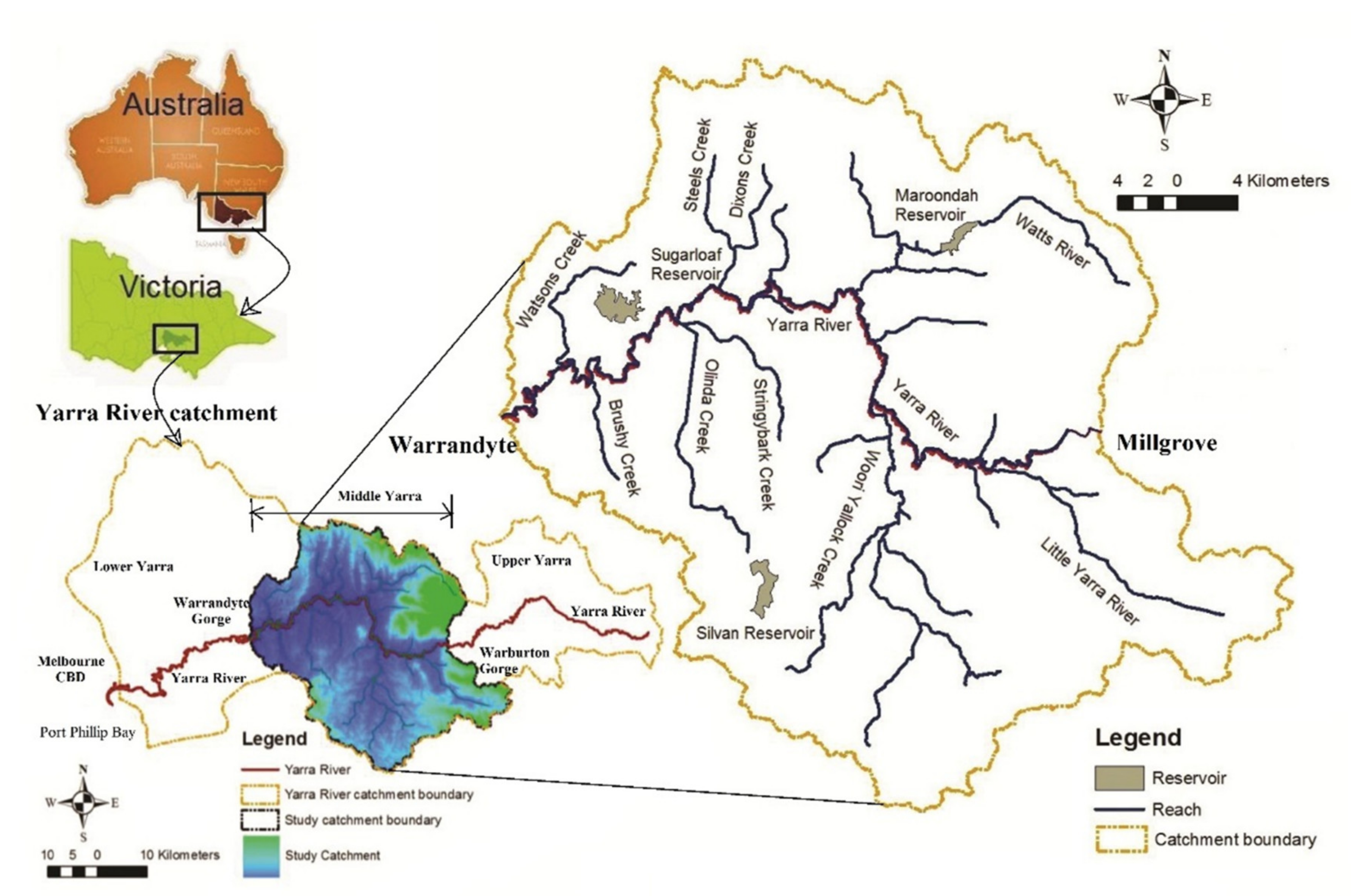
2.1. Location
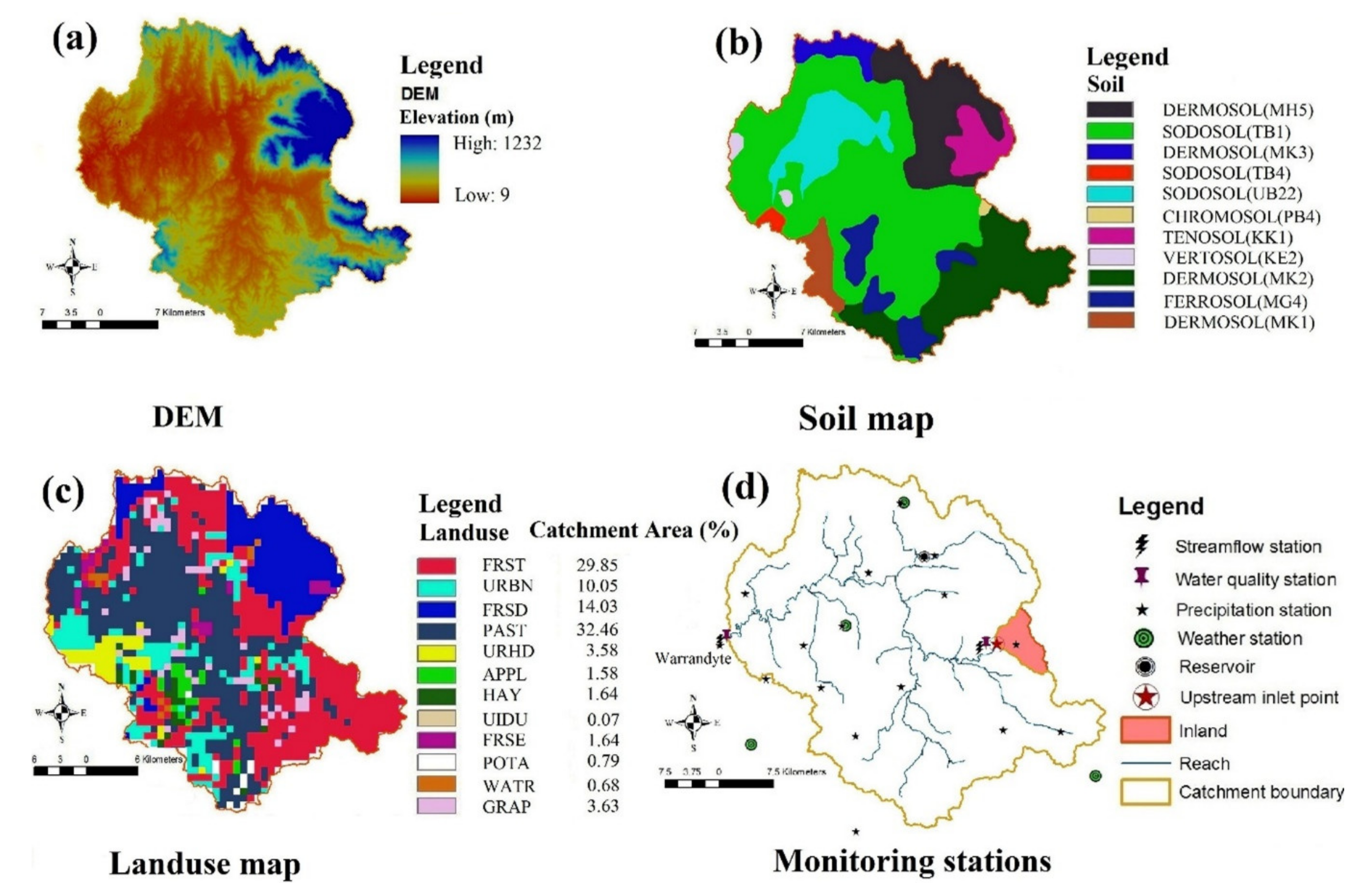
2.2. Input Data in Modelling
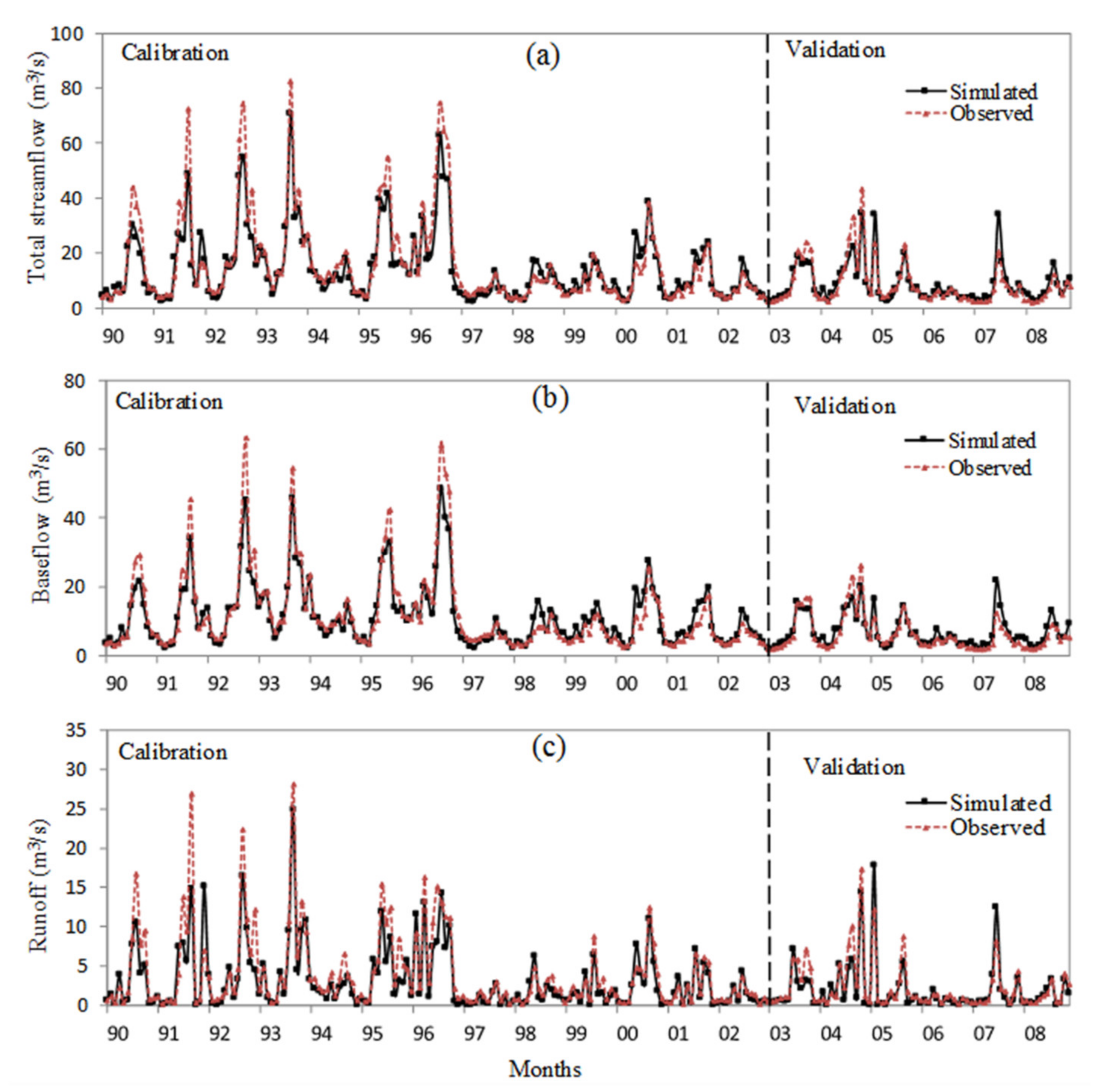
2.3. SWAT Model: Formulation, Sensitivity Analysis, Calibration, and Validation
2.4. General Circulation Models (GCMs), Future Climate Scenarios, and Projection Data
3. Results and Discussion
3.1. Model Sensitivity and Suitability
3.2. Climate Alteration Impacts on Future Rainfall and Temperature
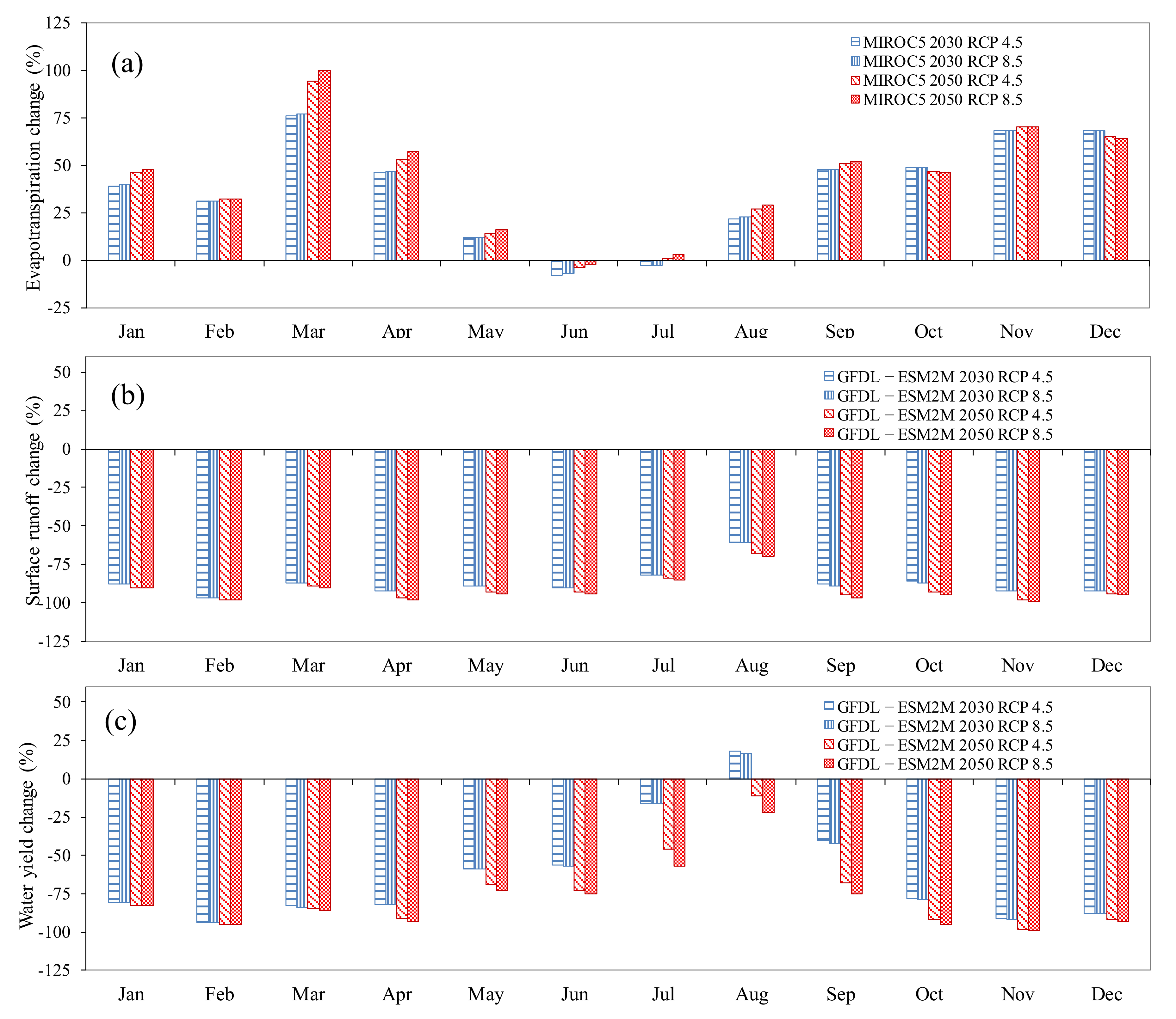
3.3. Climate Alteration Impacts on the Hydrologic Components
4. Conclusions
- Overall, the future climate projections indicate that the MYD will become hotter, with less winter–spring (June to November) rainfall and more droughts and water shortage problems in the catchment. As a result, long-term resilience and mitigation strategies are required to address the climate alteration impact on reservoir operations and water resources within the catchment study area. Such strategies may include more tree planting, rainwater harvesting, water reclamation and recycling, and efficient irrigation.
- This study demonstrated that the SWAT model can be used in Australian catchments and is a useful tool for future hydro-climatic studies, considering the uncertainties, such as recording errors, and spatial and temporal discretization in the data used for the development of the SWAT model.
- This study was conducted only for the middle agricultural part of the Yarra River catchment, and the lower urbanized and the upper forested divisions were not included in the model due to data limitations. The authors recommend further studies to be undertaken considering the Yarra River catchment as a whole to gain a complete understanding of the future impacts of climate change on the hydrology of the catchment.
- This study only used ParaSol (SCE-UA), the auto-calibration method available with the SWAT modelling tool; we recommend the use of other available calibration methods, such as the SUFI-2 method recommended by Abbaspour et al. [50,51] because during the optimization process, ParaSol (SCE-UA) assumes that the model structure is correct, and the input data is free from errors.
- In addition, an uncertainty analysis of the SWAT model is recommended to further justify its application in Australian catchments, where available data are sparse.
Author Contributions
Funding
Acknowledgments
Conflicts of Interest
Abbreviations
| List of Acronyms | |
| ASC | Australian soil classification |
| ASTER | Advanced spaceborne thermal emission and reflection radiometer |
| AWBM | Australian water balance model |
| BoM | Bureau of Meteorology |
| CMIP5 | Coupled Model Intercomparison Project, phase 5 |
| CN | Curve number |
| CO2 | Carbon dioxide |
| CSIRO | Commonwealth Scientific and Industrial Research Organisation |
| DEM | Digital elevation model |
| ET | Evapotranspiration |
| GCMs | General circulation models |
| GDEM | Global digital elevation model |
| IPCC | Intergovernmental Panel on Climate Change |
| LH-OAT | Latin-hypercube and one-factor-at-a-time |
| METI | The Ministry of Economy, Trade, and Industry (METI) of Japan |
| NASA | National Aeronautics and Space Administration |
| NSW | New South Wales |
| ParaSol | Parameter solution |
| PET | Potential evapotranspiration |
| RCP | Representative concentration pathway |
| SCE-UA | Shuffled complex evolution-The University of Arizona |
| SILO | Scientific Information for Land Owners |
| SUFI-2 | Sequential uncertainty fitting |
| SWAT | Soil and water assessment tool |
| USDA-ARS | United States Department of Agriculture-Agricultural Research Service |
Appendix A

| Name | Min | Max | Description |
|---|---|---|---|
| ALPHA_BF | 0 | 1 | Baseflow alpha factor (days) |
| CANMX | 0 | 100 | Maximum canopy storage (mm) |
| CH_K2 | −0.01 | 500 | Channel effective hydraulic conductivity (mm/h) |
| CH_N2 | −0.01 | 0.3 | Manning’s n value for main channel |
| CN2 | 35 | 98 | Initial SCS CN II value |
| EPCO | 0 | 1 | Plant uptake compensation factor |
| ESCO | 0 | 1 | Soil evaporation compensation factor |
| GW_DELAY | 0 | 500 | Groundwater delay (days) |
| GW_REVAP | 0.02 | 0.2 | Groundwater “revap” coefficient |
| GWQMN | 0 | 5000 | Threshold water depth in the shallow aquifer for flow (mm) |
| SLOPE | 0 | 0.6 | Average slope steepness (m/m) |
| SOL_AWC | 0 | 1 | Available water capacity (mm H20/mm soil) |
| SOL_K | 0 | 2000 | Saturated hydraulic conductivity (mm/h) |
| SOL_Z | 0 | 3500 | Soil depth (mm) |
| SURLAG | 1 | 24 | Surface runoff lag time (days) |
References
- IPCC. Climate Change 2007: The Physical Science Basis. Contribution of Working Group I to the Fourth Assessment Report of the Intergovernmental Panel on Climate Change; Cambridge University Press: Cambridge, UK, 2007. [Google Scholar]
- IPCC. Climate Change 2013: The Physical Science Basis. Contribution of Working Group I to the Fifth Assessment Report of the Intergovernmental Panel on Climate Change; Cambridge University Press: Cambridge, UK, 2013. [Google Scholar]
- Canadell, J.G.; Meyer, C.P.; Cook, G.D.; Dowdy, A.; Briggs, P.R.; Knauer, J.; Pepler, A.; Haverd, V. Multi-decadal increase of forest burned area in Australia is linked to climate change. Nat. Commun. 2021, 12, 6921. [Google Scholar] [CrossRef] [PubMed]
- Daloglu, I.; Cho, K.H.; Scavia, D. Evaluating causes of trends in long-term dissolved reactive phosphorus loads to Lake Erie. Environ. Sci. Technol. 2012, 46, 10660–10666. [Google Scholar] [CrossRef] [PubMed]
- Marshall, E.; Randhir, T. Effect of climate change on watershed system: A regional analysis. Clim. Chang. 2008, 89, 263–280. [Google Scholar] [CrossRef]
- Tan, M.L.; Ibrahim, A.L.; Yusop, Z.; Chua, V.P.; Chan, N.W. Climate change impacts under CMIP5 RCP scenarios on water resources of the Kelantan River Basin, Malaysia. Atmos. Res. 2017, 189, 1–10. [Google Scholar] [CrossRef]
- Samaras, A.G.; Koutitas, C.G. Modeling the impact of climate change on sediment transport and morphology in coupled watershed-coast systems: A case study using an integrated approach. Int. J. Sediment Res. 2014, 29, 304–315. [Google Scholar] [CrossRef]
- Fowler, H.J.; Blenkinsop, S.; Tebaldi, C. Linking climate change modelling to impacts studies: Recent advances in downscaling techniques for hydrological modelling. Int. J. Climatol. 2007, 27, 1547–1578. [Google Scholar] [CrossRef]
- Li, Z.; Fang, H. Impacts of climate change on water erosion: A review. Earth-Sci. Rev. 2016, 163, 94–117. [Google Scholar] [CrossRef]
- CSIRO; BoM. Climate Change in Australia Information for Australia’s Natural Resource Management Regions: Technical Report; CSIRO and Bureau of Meteorology: Melbourne, VIC, Australia, 2015. Available online: https://www.climatechangeinaustralia.gov.au/en/publications-library/technical-report/ (accessed on 25 November 2017).
- Potter, N.J.; Chiew, F.H.S.; Zheng, H.; Ekstrom, M.; Zhang, L. Hydroclimate Projections for Victoria at 2040 and 2065; CSIRO: Canberra, ACT, Australia, 2016. [Google Scholar]
- Vaze, J.; Chiew, F.H.S.; Perraud, J.M.; Viney, N.; Post, D.; Teng, J.; Wang, B.; Lerat, J.; Goswami, M. Rainfall-runoff modelling across southeast Australia: Datasets, models and results. Australas. J. Water Resour. 2011, 14, 101–116. [Google Scholar] [CrossRef]
- Boughton, W. The Australian water balance model. Environ. Model. Softw. 2004, 19, 943–956. [Google Scholar] [CrossRef]
- Chiew, F.H.S.; Peel, M.C.; Western, A.W. Application and testing of the simple rainfall-runoff model SIMHYD. In Mathematical Models of Small Watershed Hydrology and Applications; Singh, V.P., Frevert, D.K., Eds.; Water Resources Publication: Littleton, CO, USA, 2002; pp. 335–367. [Google Scholar]
- Letcher, R.A.; Jakeman, A.J.; Merritt, W.S.; McKee, L.J.; Eyre, B.D.; Baginska, B. Review of Techniques to Estimate Catchment Exports; NSW Environmental Protection Authority: Sydney, NSW, Australia, 1999.
- Howe, C.; Jones, R.N.; Maheepala, S.; Rhodes, B. Melbourne Water Climate Change Study: Implications of Potential Climate Change for Melbourne’s Water Resources; No. CMIT-2005-106; CSIRO and Melbourne Water: Melbourne, VIC, Australia, 2005. [Google Scholar]
- Post, D.A.; Chiew, F.H.S.; Teng, J.; Wang, B.; Marvanek, S. Projected Changes in Climate and Runoff for South-Eastern Australia Under 1 °C And 2 °C Of Global Warming; A SEACI Phase 2 Special Report; CSIRO: Canberra, ACT, Australia, 2012. [Google Scholar]
- Nguyen, H.H.; Recknagel, F.; Meyer, W.; Frizenschaf, J.; Shrestha, M.K. Modelling the impacts of altered management practices, land use and climate changes on the water quality of the Millbrook catchment-reservoir system in South Australia. J. Environ. Manag. 2017, 202, 1–11. [Google Scholar] [CrossRef]
- Arnold, J.G.; Srinivasan, R.; Muttiah, R.S.; Williams, J.R. Large area hydrologic modeling and assessment part I: Model development. J. Am. Water Resour. Assoc. 1998, 34, 73–89. [Google Scholar] [CrossRef]
- Borah, D.K.; Bera, M. Watershed-scale hydrologic and nonpoint-source pollution models: Review of mathematical bases. Trans. ASAE 2003, 46, 1553–1566. [Google Scholar] [CrossRef] [Green Version]
- Gassman, P.W.; Reyes, M.R.; Green, C.H.; Arnold, J.G. The soil and water assessment tool: Historical development, applications, and future research directions. Trans. ASABE 2007, 50, 1211–1250. [Google Scholar] [CrossRef] [Green Version]
- Ficklin, D.L.; Luo, Y.; Luedeling, E.; Zhang, M. Climate change sensitivity assessment of a highly agricultural watershed using SWAT. J. Hydrol. 2009, 374, 16–29. [Google Scholar] [CrossRef]
- Chen, Q.; Chen, H.; Wang, J.; Zhao, Y.; Chen, J.; Xu, C. Impacts of climate change and land-use change on hydrological extremes in the Jinsha River basin. Water 2019, 11, 1398. [Google Scholar] [CrossRef] [Green Version]
- Parajuli, P.B.; Jayakody, P.; Sassenrath, G.F.; Ouyang, Y. Assessing the impacts of climate change and tillage practices on stream flow, crop and sediment yields from the Mississippi River Basin. Agric. Water Manag. 2016, 168, 112–124. [Google Scholar] [CrossRef] [Green Version]
- Rajib, A.; Merwade, V. Hydrologic response to future land use change in the Upper Mississippi River Basin by the end of 21st century. Hydrol. Process. 2017, 31, 3645–3661. [Google Scholar] [CrossRef]
- Shrestha, M.K.; Recknagel, F.; Frizenschaf, J.; Meyer, W. Future climate and land uses effects on flow and nutrient loads of a Mediterranean catchment in South Australia. Sci. Total Environ. 2017, 590, 186–193. [Google Scholar] [CrossRef]
- Sunde, M.G.; He, H.S.; Hubbart, J.A.; Urban, M.A. Integrating downscaled CMIP5 data with a physically based hydrologic model to estimate potential climate change impacts on streamflow processes in a mixed-use watershed. Hydrol. Process. 2017, 31, 1790–1803. [Google Scholar] [CrossRef]
- Saha, P.P.; Zeleke, K. Modelling streamflow response to climate change for the Kyeamba Creek catchment of south eastern Australia. Int. J. Water 2014, 8, 241–258. [Google Scholar] [CrossRef]
- Melbourne Water and EPA Victoria. Better Bays and Waterways—A Water Quality Improvement Plan for the Port Phillip and Westernport Region; Melbourne Water and EPA Victoria: Melbourne, VIC, Australia, 2009.
- Das, S.K.; Ng, A.W.M.; Perera, B.J.C. Development of a SWAT model in the Yarra River catchment. In Proceedings of the MODSIM2013, 20th International Congress on Modelling and Simulation, Adelaide, SA, Australia, 1–6 December 2013; pp. 2457–2463, ISBN 978-0-98-721433-1. [Google Scholar] [CrossRef]
- Das, S.K.; Ng, A.W.M.; Perera, B.J.C. Sensitivity analysis of SWAT model in the Yarra River catchment. In Proceedings of the MODSIM2013, 20th International Congress on Modelling and Simulation, Adelaide, SA, Australia, 1–6 December 2013; ISBN 978-0-98-721433-1. [Google Scholar] [CrossRef]
- Winchell, M.; Srinivasan, R.; Di Luzio, M.; Arnold, J.G. ArcSWAT 2.3.4 Interface for SWAT2005 User’s Guide; Grassland, Soil and Water Research Laboratory: Temple, TX, USA, 2009.
- Borah, D.K.; Bera, M. Watershed-scale hydrologic and nonpoint-source pollution models: Review of applications. Trans. ASAE 2004, 47, 789–803. [Google Scholar] [CrossRef] [Green Version]
- Isbell, R. The Australian Soil Classification; CSIRO Publishing: Melbourne, VIC, Australia, 2002. [Google Scholar]
- Northcote, K.H. A Factual Key for The Recognition of Australian Soils, 4th ed.; Rellim Technical Publishers: Glenside, SA, Australia, 1979. [Google Scholar]
- Arnold, J.G.; Allen, P.M.; Muttiah, R.; Bernhardt, G. Automated base flow separation and recession analysis techniques. Ground Water 1995, 33, 1010–1018. [Google Scholar] [CrossRef]
- USDA-ARS. U.S. Department of Agriculture-Agricultural Research Service, Soil and Water Assessment Tool, SWAT: Baseflow Filter Program. 1999. Available online: http://swatmodel.tamu.edu/software/baseflow-filter-program (accessed on 15 November 2017).
- Van Griensven, A. Sensitivity, Auto-Calibration, Uncertainty and Model Evaluation in SWAT2005, User Guide Distributed with ArcSWAT Program. 2005. Available online: http://biomath.ugent.be/~ann/SWAT_manuals/SWAT2005_manual_sens_cal_unc.pdf (accessed on 5 November 2017).
- Moriasi, D.N.; Arnold, J.G.; Van Liew, M.W.; Bingner, R.L.; Harmel, R.D.; Veith, T.L. Model evaluation guidelines for systematic quantification of accuracy in watershed simulations. Trans. ASABE 2007, 50, 885–900. [Google Scholar] [CrossRef]
- SILO. Consistent Climate Scenarios Data. 2016. Available online: https://legacy.longpaddock.qld.gov.au/climateprojections/about.html (accessed on 10 November 2017).
- Van Griensven, A.; Meixner, T.; Grunwald, S.; Bishop, T.; Diluzio, M.; Srinivasan, R. A global sensitivity analysis tool for the parameters of multi-variable catchment models. J. Hydrol. 2006, 324, 10–23. [Google Scholar] [CrossRef]
- Gan, T.Y.; Dlamini, E.M.; Biftu, G.F. Effects of Model Complexity and Structure, Data Quality, and Objective Functions on Hydrologic Modelling. J. Hydrol. 1997, 192, 81–103. [Google Scholar] [CrossRef]
- Reckhow, K.H. Water quality simulation modelling and uncertainty analysis for risk assessment and decision making. Ecol. Model. 1994, 72, 1–20. [Google Scholar] [CrossRef]
- Arnold, J.G.; Moriasi, D.N.; Gassman, P.W.; Abbaspour, K.C.; White, M.J.; Srinivasan, R.; Santhi, C.; Harmel, R.D.; van Griensven, A.; Van Liew, M.W.; et al. SWAT: Model use, calibration, and validation. Trans. ASABE 2012, 55, 1491–1508. [Google Scholar] [CrossRef]
- Vervoort, R.W. Uncertainties in calibrating SWAT for a semi-arid catchment in NSW (Australia). In Proceedings of the 4th International SWAT Conference, Delft, The Netherlands, 2–6 July 2007. [Google Scholar]
- Watson, B.M.; Selvalingam, S.; Ghafouri, M. Evaluation of SWAT for modelling the water balance of the Woady Yaloak River catchment, Victoria. In Proceedings of the MODSIM2003: International Congress on Modelling and Simulation, Townsville, QLD, Australia, 14–17 July 2003. [Google Scholar]
- Green, C.H.; van Griensven, A. Autocalibration in hydrologic modeling: Using SWAT2005 in small-scale watersheds. Environ. Model. Softw. 2008, 23, 422–434. [Google Scholar] [CrossRef]
- Kirsch, K.; Kirsch, A.; Arnold, J.G. Predicting sediment and phosphorus loads in the Rock River basin using SWAT. Trans. ASAE 2002, 45, 1757–1769. [Google Scholar] [CrossRef]
- Hennessy, K.; Clarke, J.; Erwin, T.; Wilson, L.; Heady, C. Climate Change Impacts on Australia’s Dairy Regions; CSIRO Oceans and Atmosphere: Melbourne, VIC, Australia, 2016. [Google Scholar]
- Abbaspour, K.C.; Vejdani, M.; Haghighat, S. SWAT-CUP calibration and uncertainty programs for SWAT. In MODSIM2007: International Congress on Modelling and Simulation; Oxley, L., Kulasiri, D., Eds.; Modelling and Simulation Society of Australia and New Zealand: Christchurch, New Zealand, 2007; pp. 1603–1609. [Google Scholar]
- Abbaspour, K.C.; Yang, J.; Maximov, I.; Siber, R.; Bogner, K.; Mieleitner, J.; Zobrist, J.; Srinivasan, R. Modelling Hydrology and Water Quality in the Pre-Alpine/Alpine Thur Watershed Using SWAT. J. Hydrol. 2007, 333, 413–430. [Google Scholar] [CrossRef]


| Data | Sources |
|---|---|
| Digital elevation model (DEM) | ASTER 30 m GDEM, jointly developed by The Ministry of Economy, Trade, and Industry (METI) of Japan and the United States National Aeronautics and Space Administration (NASA), (http://asterweb.jpl.nasa.gov/gdem.asp, (accessed on 26 January 2022)). |
| Soil | Atlas of Australian Soils from the Department of Agriculture, Fisheries and Forestry, and CSIRO (http://www.asris.csiro.au, (accessed on 18 November 2021)). |
| Land use | Australian Bureau of Agricultural and Resource Economics and Sciences (50 m grid raster data for 1997 to May 2006) (http://www.agriculture.gov.au/abares/aclump/land-use, (accessed on 26 January 2022)). |
| Climate | SILO climate database (http://www.longpaddock.qld.gov.au/silo, (accessed on 15 October 2021)) and Bureau of Meteorology data for 16 precipitation/rainfall stations, and four weather stations (temperature max and min, solar radiation, wind speed, and relative humidity). |
| Streamflow | Melbourne Water (http://www.melbournewater.com.au/water-data-and-education/rainfall-and-river-levels#/, (accessed on 26 January 2022)) for daily time series data at Warrandyte (outlet of the MYD) and at Millgrove. |
| Crop management practices | Australian Bureau of Statistics (http://www.abs.gov.au, (accessed on 14 September 2021)), Melbourne Water, and the Department of Environment and Primary Industries (http://www.depi.vic.gov.au/, (accessed on 14 September 2021)) for data including tillage practices, cropping seasons, and irrigation rate. |
| Daily | Monthly | Annual | |||||||||||
|---|---|---|---|---|---|---|---|---|---|---|---|---|---|
| R2 | NSE | PBIAS | RSR | R2 | NSE | PBIAS | RSR | R2 | NSE | PBIAS | RSR | ||
| Total streamflow | Calibration | 0.78 | 0.77 | 10 | 0.48 | 0.93 | 0.89 | 10 | 0.34 | 0.96 | 0.87 | 10 | 0.36 |
| Validation | 0.74 | 0.72 | −3 | 0.53 | 0.82 | 0.82 | −3 | 0.43 | 0.87 | 0.81 | −3 | 0.43 | |
| Baseflow | Calibration | 0.90 | 0.87 | 6 | 0.36 | 0.93 | 0.89 | 6 | 0.33 | 0.95 | 0.88 | 6 | 0.35 |
| Validation | 0.79 | 0.77 | −11 | 0.48 | 0.81 | 0.79 | −11 | 0.46 | 0.84 | 0.71 | −11 | 0.54 | |
| Runoff | Calibration | 0.50 | 0.42 | 23 | 0.76 | 0.84 | 0.80 | 23 | 0.45 | 0.97 | 0.76 | 23 | 0.49 |
| Validation | 0.67 | 0.53 | 19 | 0.69 | 0.82 | 0.79 | 19 | 0.46 | 0.87 | 0.70 | 19 | 0.55 | |
| ACCESS1-0 RCP 4.5 | CanESM2 RCP 4.5 | CNRM-CM5 RCP 4.5 | GFDL-ESM2M RCP 4.5 | MIROC5 RCP 4.5 | ACCESS1-0 RCP 8.5 | CanESM2 RCP 8.5 | CNRM-CM5 RCP 8.5 | GFDL-ESM2M RCP 8.5 | MIROC5 RCP 8.5 | |||||||||||
|---|---|---|---|---|---|---|---|---|---|---|---|---|---|---|---|---|---|---|---|---|
| P(%) | T(°C) | P(%) | T(°C) | P(%) | T(°C) | P(%) | T(°C) | P(%) | T(°C) | P(%) | T(°C) | P(%) | T(°C) | P(%) | T(°C) | P(%) | T(°C) | P(%) | T(°C) | |
| Jan. | −1 | 1.2 | 18 | 1.5 | −1 | 1.4 | −3 | 1.3 | 4 | 1.0 | −1 | 1.2 | 19 | 1.5 | −1 | 1.5 | −3 | 1.3 | 4 | 1.0 |
| Feb. | −12 | 1.1 | 0 | 1.4 | 6 | 1.2 | −7 | 1.4 | 0 | 1.0 | −13 | 1.1 | 0 | 1.4 | 6 | 1.2 | −7 | 1.4 | 0 | 1.0 |
| Mar. | −13 | 1.4 | 1 | 1.5 | −8 | 1.8 | −3 | 1.3 | 15 | 0.8 | −13 | 1.5 | 1 | 1.6 | −8 | 1.9 | −4 | 1.4 | 15 | 0.8 |
| Apr. | −3 | 1.4 | 5 | 1.5 | 8 | 1.4 | −21 | 1.6 | 15 | 1.3 | −3 | 1.5 | 5 | 1.5 | 8 | 1.4 | −21 | 1.6 | 16 | 1.3 |
| May | −18 | 1.3 | 4 | 1.3 | 6 | 1.2 | −11 | 1.2 | 5 | 1.1 | −18 | 1.3 | 4 | 1.3 | 6 | 1.2 | −11 | 1.3 | 5 | 1.1 |
| Jun. | −6 | 1.3 | −2 | 1.0 | −9 | 0.9 | −14 | 1.0 | 4 | 1.2 | −6 | 1.3 | −2 | 1.1 | −10 | 0.9 | −15 | 1.1 | 4 | 1.2 |
| Jul. | −3 | 1.3 | 0 | 1.1 | −9 | 1.0 | −7 | 1.2 | 3 | 1.1 | −3 | 1.3 | 0 | 1.1 | −9 | 1.0 | −7 | 1.2 | 3 | 1.1 |
| Aug. | −3 | 1.1 | −2 | 1.2 | −9 | 1.0 | −9 | 1.2 | 2 | 1.0 | −3 | 1.2 | −2 | 1.2 | −9 | 1.1 | −10 | 1.2 | 2 | 1.0 |
| Sep. | −16 | 1.1 | −1 | 1.2 | −9 | 1.3 | −25 | 1.2 | −5 | 0.9 | −17 | 1.2 | −1 | 1.2 | −10 | 1.4 | −25 | 1.2 | −5 | 0.9 |
| Oct. | −17 | 1.4 | −9 | 1.3 | −15 | 1.4 | −20 | 2.0 | −10 | 1.2 | −17 | 1.4 | −9 | 1.3 | −15 | 1.5 | −20 | 2.0 | −10 | 1.2 |
| Nov. | −13 | 1.4 | −12 | 1.6 | −8 | 1.5 | −30 | 2.0 | 1 | 1.2 | −13 | 1.4 | −12 | 1.7 | −8 | 1.6 | −31 | 2.1 | 1 | 1.2 |
| Dec. | 3 | 1.3 | −4 | 1.8 | −17 | 1.5 | −12 | 1.9 | −1 | 1.1 | 3 | 1.3 | −4 | 1.8 | −18 | 1.6 | −13 | 1.9 | −1 | 1.1 |
| Year | −8 | 1.3 | 0 | 1.4 | −6 | 1.3 | −14 | 1.4 | 3 | 1.1 | −9 | 1.3 | 0 | 1.4 | −6 | 1.3 | −14 | 1.5 | 3 | 1.1 |
| ACCESS1-0 RCP 4.5 | CanESM2 RCP 4.5 | CNRM-CM5 RCP 4.5 | GFDL-ESM2M RCP 4.5 | MIROC5 RCP 4.5 | ACCESS1-0 RCP 8.5 | CanESM2 RCP 8.5 | CNRM-CM5 RCP 8.5 | GFDL-ESM2M RCP 8.5 | MIROC5 RCP 8.5 | |||||||||||
|---|---|---|---|---|---|---|---|---|---|---|---|---|---|---|---|---|---|---|---|---|
| P(%) | T(°C) | P(%) | T(°C) | P(%) | T(°C) | P(%) | T(°C) | P(%) | T(°C) | P(%) | T(°C) | P(%) | T(°C) | P(%) | T(°C) | P(%) | T(°C) | P(%) | T(°C) | |
| Jan. | −2 | 2.1 | 33 | 2.6 | −1 | 2.6 | −6 | 2.3 | 7 | 1.8 | −2 | 2.5 | 39 | 3.1 | −1 | 3.0 | −7 | 2.7 | 9 | 2.1 |
| Feb. | −22 | 2.0 | 1 | 2.4 | 10 | 2.1 | −13 | 2.5 | 0 | 1.7 | −26 | 2.3 | 1 | 2.9 | 12 | 2.5 | −15 | 2.9 | 1 | 2.0 |
| Mar. | −23 | 2.5 | 2 | 2.7 | −15 | 3.2 | −6 | 2.4 | 27 | 1.5 | −27 | 3.0 | 2 | 3.2 | −17 | 3.8 | −7 | 2.8 | 32 | 1.7 |
| Apr. | −5 | 2.5 | 8 | 2.6 | 14 | 2.5 | −37 | 2.9 | 27 | 2.3 | −6 | 3.0 | 10 | 3.0 | 16 | 2.9 | −43 | 3.4 | 32 | 2.7 |
| May | −32 | 2.3 | 7 | 2.2 | 11 | 2.1 | −19 | 2.2 | 9 | 2.0 | −37 | 2.7 | 9 | 2.6 | 13 | 2.5 | −23 | 2.6 | 10 | 2.3 |
| Jun. | −11 | 2.3 | −4 | 1.8 | −17 | 1.6 | −26 | 1.9 | 8 | 2.2 | −13 | 2.7 | −5 | 2.2 | −20 | 1.9 | −30 | 2.2 | 9 | 2.5 |
| Jul. | −5 | 2.2 | 0 | 1.9 | −16 | 1.8 | −12 | 2.1 | 6 | 1.9 | −6 | 2.6 | 0 | 2.3 | −19 | 2.1 | −15 | 2.5 | 7 | 2.2 |
| Aug. | −5 | 2.0 | −4 | 2.1 | −16 | 1.8 | −17 | 2.2 | 3 | 1.7 | −5 | 2.4 | −4 | 2.5 | −19 | 2.2 | −20 | 2.5 | 4 | 2.0 |
| Sep. | −29 | 2.0 | −1 | 2.0 | −17 | 2.4 | −44 | 2.1 | −9 | 1.6 | −34 | 2.4 | −1 | 2.4 | −20 | 2.8 | −52 | 2.4 | −10 | 1.8 |
| Oct. | −30 | 2.4 | −16 | 2.3 | −26 | 2.5 | −36 | 3.5 | −17 | 2.1 | −35 | 2.9 | −19 | 2.7 | −31 | 3.0 | −42 | 4.2 | −21 | 2.4 |
| Nov. | −23 | 2.4 | −21 | 2.9 | −14 | 2.7 | −53 | 3.6 | 1 | 2.1 | −27 | 2.8 | −25 | 3.4 | −16 | 3.2 | −62 | 4.2 | 2 | 2.5 |
| Dec. | 6 | 2.3 | −7 | 3.2 | −31 | 2.7 | −22 | 3.3 | −2 | 1.9 | 7 | 2.7 | −9 | 3.7 | −36 | 3.2 | −26 | 3.9 | −2 | 2.2 |
| Year | −15 | 2.3 | 0 | 2.4 | −10 | 2.3 | −24 | 2.6 | 5 | 1.9 | −18 | 2.7 | 0 | 2.8 | −12 | 2.8 | −28 | 3.0 | 6 | 2.2 |
| Years | RCPs | GCMs | RAIN | ET | SW | SURQ | LATQ | GWQ | WYLD |
|---|---|---|---|---|---|---|---|---|---|
| 2030 | RCP4.5 | ACCESS1-0 | −8 | 33 | −2 | −84 | −23 | −21 | −41 |
| CanESM2 | 0 | 40 | 2 | −81 | −12 | 4 | −27 | ||
| CNRM-CM5 | −6 | 34 | 0 | −84 | −19 | −10 | −35 | ||
| GFDL-ESM2M | −14 | 28 | −9 | −87 | −32 | −37 | −51 | ||
| MIROC5 | 3 | 41 | 6 | −80 | −6 | 19 | −19 | ||
| RCP8.5 | ACCESS1-0 | −9 | 33 | −3 | −84 | −24 | −22 | −41 | |
| CanESM2 | 0 | 40 | 2 | −81 | −12 | 4 | −27 | ||
| CNRM-CM5 | −6 | 34 | −1 | −84 | −20 | −11 | −36 | ||
| GFDL-ESM2M | −14 | 27 | −9 | −87 | −33 | −38 | −52 | ||
| MIROC5 | 3 | 42 | 6 | −80 | −6 | 19 | −19 | ||
| 2050 | RCP4.5 | ACCESS1-0 | −15 | 28 | −11 | −87 | −34 | −44 | −54 |
| CanESM2 | 0 | 42 | −2 | −82 | −15 | −4 | −31 | ||
| CNRM-CM5 | −10 | 31 | −6 | −86 | −28 | −28 | −46 | ||
| GFDL-ESM2M | −24 | 15 | −21 | −91 | −48 | −65 | −68 | ||
| MIROC5 | 5 | 45 | 4 | −79 | −5 | 22 | −17 | ||
| RCP8.5 | ACCESS1-0 | −18 | 25 | −15 | −88 | −38 | −52 | −59 | |
| CanESM2 | 0 | 43 | −3 | −82 | −16 | −7 | −33 | ||
| CNRM-CM5 | −12 | 29 | −9 | −87 | −31 | −35 | −50 | ||
| GFDL-ESM2M | −28 | 8 | −26 | −93 | −53 | −73 | −73 | ||
| MIROC5 | 6 | 46 | 3 | −79 | −5 | 23 | −16 |
Publisher’s Note: MDPI stays neutral with regard to jurisdictional claims in published maps and institutional affiliations. |
© 2022 by the authors. Licensee MDPI, Basel, Switzerland. This article is an open access article distributed under the terms and conditions of the Creative Commons Attribution (CC BY) license (https://creativecommons.org/licenses/by/4.0/).
Share and Cite
Das, S.K.; Ahsan, A.; Khan, M.H.R.B.; Tariq, M.A.U.R.; Muttil, N.; Ng, A.W.M. Impacts of Climate Alteration on the Hydrology of the Yarra River Catchment, Australia Using GCMs and SWAT Model. Water 2022, 14, 445. https://doi.org/10.3390/w14030445
Das SK, Ahsan A, Khan MHRB, Tariq MAUR, Muttil N, Ng AWM. Impacts of Climate Alteration on the Hydrology of the Yarra River Catchment, Australia Using GCMs and SWAT Model. Water. 2022; 14(3):445. https://doi.org/10.3390/w14030445
Chicago/Turabian StyleDas, Sushil K., Amimul Ahsan, Md. Habibur Rahman Bejoy Khan, Muhammad Atiq Ur Rehman Tariq, Nitin Muttil, and Anne W. M. Ng. 2022. "Impacts of Climate Alteration on the Hydrology of the Yarra River Catchment, Australia Using GCMs and SWAT Model" Water 14, no. 3: 445. https://doi.org/10.3390/w14030445