Has Technological Progress Contributed to the Bias of Green Output in China’s Marine Economy?

Abstract

At present, the destruction of the marine ecological environment and the imbalance of economic structure have put forward urgent requirements for the green development of the marine economy. Based on the input and output data of China’s coastal provinces from 2006 to 2018, the RDM (range directional model) direction distance function was used to measure the output bias technology progress (OBTC) index of each region, and its influence on China’s marine economy green total factor productivity (GTFP) was judged accordingly. Furthermore, the rationality of the current OBTC index was studied. The results show that there is obvious output-biased technological progress in China’s marine economy, and it has led to the improvement of the GTFP. Although most coastal areas still tend to pursue the improvement of the total output value of the marine economy at the expense of environmental damage, the green bias of China’s marine economy has improved significantly since 2015, driven by relevant marine environmental protection policies. From the perspective of different areas, the imbalance of regional development in the process of China’s marine economic development is significant. The green bias of the marine economy is highest in the East China Sea area and lowest in the Bohai rim area. However, the coordination between the development of the green marine economy and environmental protection in the South China Sea area needs to be improved.

1. Introduction

In the past ten years, the growth rate of China’s marine economy has been higher than that of the national economy in the same period, with the gross ocean product (GOP) at the end of the 12th Five-Year Plan reaching 6466.9 billion yuan. China’s marine economy is becoming more and more important in the national economy. However, at the same time, a series of problems such as the destruction of marine ecological environment, the imbalance of economic structures, and the expansion of spatial differences have emerged [1]. It shows an extensive development of “high energy consumption and low output” [2]. In this regard, the 2012 report of the 18th National Congress of the Communist Party of China (hereinafter Report) proposed to improve the capacity of marine resources’ exploitation and protect the ecological environment. The policy reflects the urgent need for green development of the marine economy, which means that related industries are required to adjust production in the direction of reducing environmental damage [3]. However, the gap between the regions in green development is large, and coordination is insufficient, which is not conducive to the steady development of the marine economy [4,5]. The key to improving the equilibrium of green marine economic development between regions lies in making clear the regions’ objective conditions and comparative advantages, and accordingly, formulating local development strategies, rationally allocating various factors of production, and highlighting their own development priorities to promote the coordinated development of the regions.

The development of marine economy is inseparable from various inputs [6], and the impact of inputs on outputs is two-sided. When the desirable output is obtained, it inevitably results, in part, in an undesirable output, namely marine pollution [7]. It has led to the loss of living marine resources and the deterioration of marine sites [8,9]. With the depletion of marine resources and the increasing input of marine industry, the sustainable growth of the marine economy is facing serious challenges, which put forward higher demands on the efficiency of green output [10,11]. Improving the efficiency of green output is to enhance the role of technological progress on desirable output and reduce the proportion of undesirable output, which reflects the degree of green bias of marine economic development. It can be seen that the bias of technological progress from the output perspective is the main reason for the uneven degree of green bias, which has a very important impact on the sustainable development of the marine economy.

At present, the research on the biased technological progress of China’s marine economy mainly has focused on the impact of capital, labor, and resources on marine economic growth, that is, from the perspective of input, to analyze the sources of China’s uneven marine economic development [12,13,14]. However, there is little research that explores whether the current process of China’s marine economic development is in harmony with the protection of the ecological environment from the perspective of output. Exploring the green growth of marine economy from the output perspective can more intuitively reflect the difference in the degree of green bias. Measuring the degree of green bias of the output in different areas is conducive to the implementation of environmental protection measures adapted to local conditions, which can improve the effective output efficiency, promote interregional coordinated development, and promote the high-quality development of China’s marine economy.

Since the 21st century, the connotation of sustainable development has been continuously enriched [15,16,17,18,19], however, with the further depletion of land resources, the development of the marine economy has become a new hot spot in global economic development [20,21,22]. Giving full play to the leading role of technological progress in the bias of green output, reducing marine environmental pollution and enhancing the total output value of the ocean are important requirements for the marine technological progress of the present sustainable development goals. Exploring the degree of coordination between technological progress and the bias of green output in the marine economy is the starting point of this paper. This work makes the following main contributions to the existing literature by:

• using the directional distance function based on RDM, the Chinese marine GTFP was measured and decomposed to obtain the OBTC index of each coastal province from 2006 to 2018, to judge whether there is obvious output-biased technological progress in the development process of China’s marine economy.
• analyzing the rationality of the current output-biased technological progress, and judging whether the technological progress of each province in each year has promoted the green output bias of China’s marine economy from the two dimensions of time and space, and then identifying the non-efficient areas and providing guidance for them to improve the input–output structure and optimize resource allocation.

2. Materials and Methods

2.1. Study Area

The total area of China’s four major seas is more than 4.7 million square kilometers, spanning 32 longitudes of east to west and 44 latitudes from north to south. The mainland coastline, from the Yalu River estuary in Liaoning province to Beilun Estuary in Guangxi, has a total length of 18,000 km, ranking fourth in the world. In China, there are more than 6960 islands, large and small, with a total island area of nearly 80,000 square kilometers and a total island coastline of about 14,000 km. Rich marine resources and good location advantages are the superior basic conditions for the rapid development of the marine economy [23].

2.2. Methods

2.2.1. Nonparametric Methods Based on the DEA (Data Envelopment Analysis)

At present, the measurement method of biased technological progress is mainly divided into the parameter method and non-parameter method. The former is mostly based on pre-determined forms of production functions, estimating the alternative elasticity between factors, and using them as a basis for analyzing the bias of technological progress [24,25]. The latter is represented by the DEA method [26,27], which does not require the designation of a special form of production function, avoiding the estimated deviation due to pre-determined production functions. In addition, the parameter method also needs input and output variable price data, but the pollutant price data collection is difficult, and pricing by external influence is not necessarily reasonable. Therefore, the strict measurement conditions of the parametric method make it difficult to achieve. However, the nonparametric method only needs to set input and output variables, and the measurement conditions are easy to satisfy [28]. In addition, unlike the parameter method, the DEA model can solve the problem of multi-input and multi-output and has been used in many fields [29,30,31,32]. In a word, the non-parametric method based on DEA was more operable and suitable for this study.

Specifically, this paper used the DEA method to measure the green Malmquist-Luenberger (ML) index and then used this index to represent the change in GTFP. Then, referring to Fare’s approach [33], the GTFP index was broken down into two parts, the technology change (TC) index and the technology efficiency change (EC) index, wherein the former can be broken down into the input-biased technological progress (IBTC) index, OBTC index, and technology scale change (MATC) index. Finally, based on the research of Weber and Dominzlicky [34], the paper compared the OBTC index with the cross-period change of output combination, to judge the output bias of marine technology; that is, whether marine technology is biased towards reducing pollution emissions and provides a basis for further discussion of the relationship between marine resources, environment, and development in China.

2.2.2. The Direction Distance Function Based on the RDM

Traditional DEA models cannot process data sets that contain undesirable outputs, i.e., pollution of the marine environment, as undesirable output makes it more difficult to measure productivity growth. Therefore, to solve this problem, this paper refers to the method of Portela et al. [35] and improved the direction distance function based on RDM. This function can evaluate a data set containing undesirable outputs (e.g., marine wastewater, marine exhaust gas, marine solid waste) with the advantages of unit invariance, translational invariance, and the improvement of the invalid unit, with it being closer to the effective frontier. In particular, the direction vector of RDM is the possible improvement of the decision-making unit, which does not change the original undesirable output data, and improves the authenticity and reliability of the efficiency estimation results [36].

In this paper, the marine production of each coastal province was regarded as the decision-making unit, and the following definition was made: the decision-making unit set is $J=\left\{1,\cdots ,n\right\}$, the input vector of the m marine production factors of the estimated unit K is $x_{ij}=\left(x_{1j}^t,\cdots ,x_{mj}^t\right)\in R^{+}$, the output vector includes $p$ desirable outputs and $q$ undesirable outputs $y_{b_v}=\left(y_{b_{1}j}^t,\cdots ,y_{b_{q}j}^t\right)\in R^{+}$, $p+q=s$. $g^t=\left(g_x^t,g_y^t\right)$ is a set of vectors that reflect the direction of change in input and output. RDM sets the combination of minimum input and maximum output for the t-period as the ideal point IP, which satisfies $I{P}_i^t=\underset{J}{min}\left\{x_{ij}^t\right\}$, $i=1,\cdots ,m$ for input $x_i$, $I{P}_{g_u}=\underset{J}{max}\left\{y_{g_{u}j}^t\right\}$, $u=1,\cdots ,p$ for output $y_{g_u}$, $I{P}_{b_v}=\underset{J}{min}\left\{y_{b_{v}j}^t\right\}$, $v=1,\cdots ,q$ for output $y_{b_v}$. The direction vector based on the RDM can then be expressed as:

$$\left(g_x^t,g_y^t\right)=\left(R_x^t,R_{y_g}^t,-R_{y_b}^t\right)=\left(R_{x_1}^t,\cdots ,R_{x_m}^t,R_{y_{g_1}}^t,\cdots ,R_{y_{g_p}}^t,-R_{y_{b_1}}^t,\cdots ,-R_{y_{b_q}}^t\right)$$

where $R_x^t=x_i^t-\underset{j}{min}\left\{x_{ij}^t\right\}$, ${\hat{R}}_{y_g}^t=\underset{j}{max}\left\{y_{g_{u}j}^t\right\}-y_{g_u}^t$, $R_{yb}^t=y_{b_v}^t-\underset{J}{min}\left\{y_{b_{v}j}^t\right\}$. Thus, the RDM directional distance function can be obtained as:

$${\overrightarrow{D}}^t\left(x^t,y_g^t,y_b^t;R_x^t,R_{y_g^t},-R_{y_b^t}\right)=sup\left\{\beta :x^t-\beta R_{x^t},y_g^t+\beta R_{y_g^t},y_b^t-\beta R_{y_b^t}\right\}$$

(1)

2.2.3. Measurement of the OBTC Index

When the input is given, the output distance function describes the characteristics of the production technique by comparing the changes brought about by the expansion of the maximum proportion of each output combination. Assuming that the output that reflects technological changes may be set to $p^t\left(x\right)=\left\{\left(y_g,y_b\right):x \mathrm{can} \mathrm{produce} \left(y_g,y_b\right)\right\}$, the RDM output distance function can be expressed as: ${\overrightarrow{D}}_o^t\left(x^t,y_g^t,y_b^t;R_{y_g^t},-R_{y_b^t}\right)=sup\left\{\beta :y_g^t+\beta R_{y_g^t}\in \right.\left.p^t\left(x\right),y_b^t-\beta R_{y_b^t}\in p^t\left(x\right)\right\}.$

Then, the output technical efficiency value of the decision-making unit $DM{U}_k$ can be obtained by solving the following linear planning problems that meet the constraints of constant scale compensation:

$$\begin{array}{l}{\overrightarrow{D}}_o^t\left(x^t,y_g^t,y_b^t;R_{y_g^t}\right)=max\{{\beta }_k\mid {\Sigma }_{j=1}^n z_j^t{x}_{ij}^t\le x_{ik}^t,i=1,\cdots ,m\\ {\Sigma }_{j=1}^n z_j^t{y}_{g_{w}j}^t\ge y_{g_{u}k}^t+{\beta }_k{R}_{y_{guk}^t},u=1,\cdots ,p\\ {\Sigma }_{j=1}^n z_j^t{y}_{b_{v}j}^t\le y_{b_{v}k}^t-{\beta }_k{R}_{y_{bv}^t},v=1,\cdots ,q\\ {\Sigma }_{j=1}^n z_j^t=1,z_j^t\ge 0\end{array}$$

(2)

Then, using the methods of Chung et al. [37], based on the Malmquist index model, the distance function containing undesirable output is considered to construct the ML index. At a certain input, $D_o^t\left(y_g^t,y_b^t,x^t;R_{y_g^t},-R_{y_b^t}\right)$ and $D_o^{t+1}\left(y_g^{t+1},y_b^{t+1},x^{t+1};R_{y_g^t},-R_{y_b^t}\right)$ represent the direction distance functions of period $t$ and period $t+1$, respectively, when $R_x$ = 0. The ML index decomposition method is used to measure a series of indicators. The model is as follows:

$$ML=\sqrt{\frac{D_i^{t+1}\left(y_g^{t+1},y_b^{t+1},x^{t+1};R_{y_g^t},-R_{y_b^t}\right)}{D_i^{t+1}\left(y_g^t,y_b^t,x^t;R_{y_g^t},-R_{y_b^t}\right)}\times \frac{D_i^t\left(y_g^{t+1},y_b^{t+1},x^{t+1};R_{y_g^t},-R_{y_b^t}\right)}{D_i^t\left(y_g^t,y_b^t,x^t;R_{y_g^t},-R_{y_b^t}\right)}}$$

(3)

Decomposition then obtains:

$$ML=EC\times TC=\frac{D_i^{t+1}\left(y_g^{t+1},y_b^{t+1}{x}^{t+1};R_{y_g^t},-R_{y_b^t}\right)}{D_i^t\left(y_g^t,y_b^t,x^t;R_{y_g^t},-R_{y_b^t}\right)}\times \sqrt{\frac{D_i^t\left(y_g^t,y_b^t,x^t;R_{y_g^t},-R_{y_b^t}\right)}{D_i^{t+1}\left(y_g^t,y_b^t,x^t;R_{y_g^t},-R_{y_b^t}\right)}\times \frac{D_i^t\left(y_g^{t+1},y_b^{t+1},x^{t+1};R_{y_g^t},-R_{y_b^t}\right)}{D_i^{t+1}\left(y_g^{t+1},y_b^{t+1},x^{t+1};R_{y_g^t},-R_{y_b^t}\right)}}$$

(4)

Using the method of Fare et al. [34], the TC index is further decomposed to obtain the neutral technology progress index and the biased technology progress index:

$$MATC=\frac{D_i^t\left(y_g^t,y_b^t,x^t;R_{y_g^t},-R_{y_b^t}\right)}{D_i^{t+1}\left(y_g^t,y_b^t,x^t;R_{y_g^t},-R_{y_b^t}\right)}$$

(5)

$$IBTC=\sqrt{\frac{D_i^{t+1}\left(y_g^t,y_b^t,x^t;R_{y_g^t},-R_{y_b^t}\right)}{D_i^t\left(y_g^t,y_b^t,x^t;R_{y_g^t},-R_{y_b^t}\right)}\times \frac{D_i^t\left(y_g^t{y}_b^t,x^{t+1};R_{y_g^t},-R_{y_b^t}\right)}{D_i^{t+1}\left(y_g^t,y_b^t,x^{t+1};R_{y_g^t},-R_{y_b^t}\right)}}$$

(6)

$$OBTC=\sqrt{\frac{D_i^t\left(y_g^{t+1},y_b^{t+1},x^{t+1};R_{y_g^{t+1}},-R_{y_b^{t+1}}\right)}{D_i^{t+1}\left(y_g^{t+1},y_b^{t+1},x^{t+1};R_{y_g^{t+1}},-R_{y_b^{t+1}}\right)}\times \frac{D_i^{t+1}\left(y_g^t{y}_b^t,x^{t+1};R_{y_g^t},-R_{y_b^t}\right)}{D_i^t\left(y_g^t,y_b^t,x^{t+1};R_{y_g^t},-R_{y_b^t}\right)}}$$

(7)

And TC = MATC × IBTC ×OBTC.

With constant returns to scale, Shephard’s input distance function is equal to the reciprocal of output distance function [35], i.e.,

$$D_i^t\left(y_g^t,y_b^t,x^t\right)=D_0^t{\left(x^t,y_g^t,y_b^t\right)}^{-1}$$

(8)

An output oriented OBTC index is computed as follows:

$$OBTC=\sqrt{\frac{D_0^t\left(x^{t+1},y_g^{t+1},y_b^{t+1};R_{y_g^{t+1}},-R_{y_b^{t+1}}\right)}{D_o^{t+1}\left(x^{t+1},y_g^{t+1},y_b^{t+1};R_{y_g^{t+1}},-R_{y_b^{t+1}}\right)}\times \frac{D_o^{t+1}\left(x^{t+1},y_g^t,y_b^t;R_{y_g^t},-R_{y_b^t}\right)}{D_0^t\left(x^{t+1},y_g^t,y_b^t;R_{y_g^t},-R_{y_b^t}\right)}}$$

(9)

Among them, OBTC in the Formula (9) reflects the bias promotion effect of technological progress on different outputs, that is, the calculation formula of the OBTC index in this paper. When there is only one output, the value of the index is always 1 [38].

In the above formula, the ML, EC, TC, MATC, IBTC, and OBTC indices all represent the rate of change between period $t$ and $t+1$. The change rate index is greater than (less than) 1, indicating that the indicator is larger (decrease) than the previous period.

2.2.4. The Method of Judging Output Bias

Figure 1 shows the principle of identification of the output bias of technological progress. In this paper, two output indicators (desirable output is the value added of the marine industry and undesirable output is marine pollutant emission index) were constructed in the model, represented by the letters $y_g$, and $y_b$ respectively. In Figure 1, $P^1\left(x\right)$ represents the production probability curve for period $t_1$, and $P^2\left(x\right)$ represents the outflow of the output probability curve for period $t_2$, which is Hicks-neutral, given that the marginal rate of transformation (MRT) of two outputs remains constant. Direction vectors $g^{t1}$ and $g^{t2}$ indicate the direction in which output-biased technological progress has contributed to the improvement of economic production (increase desirable output $y_g$, reduce undesired output $y_b$) in two periods, respectively.

If the MRT of $y_g$ to $y_b$ increases from period $t_1$ to period $t_2$, then the technological progress in output will be biased towards production $y_g$, which, in the Figure, can be shown as $P^1\left(x\right)$ moving to $P^4\left(x\right)$. Similarly, from period $t_1$ to period $t_2$, the MRT of $y_g$ to $y_b$ decreases, then, the technological progress of the output will be biased towards production $y_b$, shown in the Figure as $P^1\left(x\right)$ moving to $P^3\left(x\right)$.

The following is an example of how to judge the bias of a particular output. If point A represents an inefficient combination of outputs in period $t_1$, and points B and C intersect with $P^1\left(x\right)$ and $P^4\left(x\right)$ by rays passing through points O and A, respectively, the output direction distance function value is ${\overrightarrow{D}}_o^1\left(x^{t1},y_g^{t1};g^{t1}\right)=\frac{OB}{OA}$. In period $t_2$, it is assumed that the output combination point is F and that the set of production possibilities becomes $P^4\left(x\right)$, and points E and G intersect with $P^1\left(x\right)$ and $P^4\left(x\right)$ by rays passing through points O and F, respectively. Point F is below the $l_1$ curve, so the $MR{T}_{gb}$ (The ratio of desirable and undesirable outputs across periods) is less than 1, i.e., $\frac{y_g^{t+1}}{y_b^{t+1}}<\frac{y_g^t}{y_b^t}$. According to Formula (9), the output distance function value is ${\overrightarrow{D}}_o^2\left(x^{t2},y_g^{t2};g^{t2}\right)=\frac{OG}{OF}$. The values are substituted for equations and OBTC = $\sqrt{\frac{OE/OF}{OG/OF}\times \frac{OC/OA}{OB/OA}}=\sqrt{\frac{OE/OG}{OB/OC}}>1$. When combined with the $P^4\left(x\right)$ curve moving in the direction of fit $y_g$, it can be concluded that when OBTC $>$ 1 and $MR{T}_{gb}<1$ ($MR{T}_{bg}>1$), with output-biased technological progress towards producing $y_g$. When combined with this law, this paper obtained the bias direction of technological progress to different outputs by calculating the MRT and the OBTC value, which was calculated by software.

When combining the cross-period changes of marine inputs and outputs with the corresponding OBTC index, the specific bias determination rules of output-biased technological progress in

Table 1. The method of judging output bias.

Output Mix	OBTC > 1	OBTC = 1	OBTC < 1
$\frac{y_g^{t+1}}{y_b^{t+1}}<\frac{y_g^t}{y_b^t}$	$y_g$	neutrality	$y_b$
$\frac{y_g^{t+1}}{y_b^{t+1}}>\frac{y_g^t}{y_b^t}$	$y_b$	neutrality	$y_g$

were obtained, i.e., the basis for determining whether technological progress is biased towards environmental protection ($y_g$ for value added of GOP, $y_b$ for marine economic pollutant emissions):

2.3. Data Acquisition

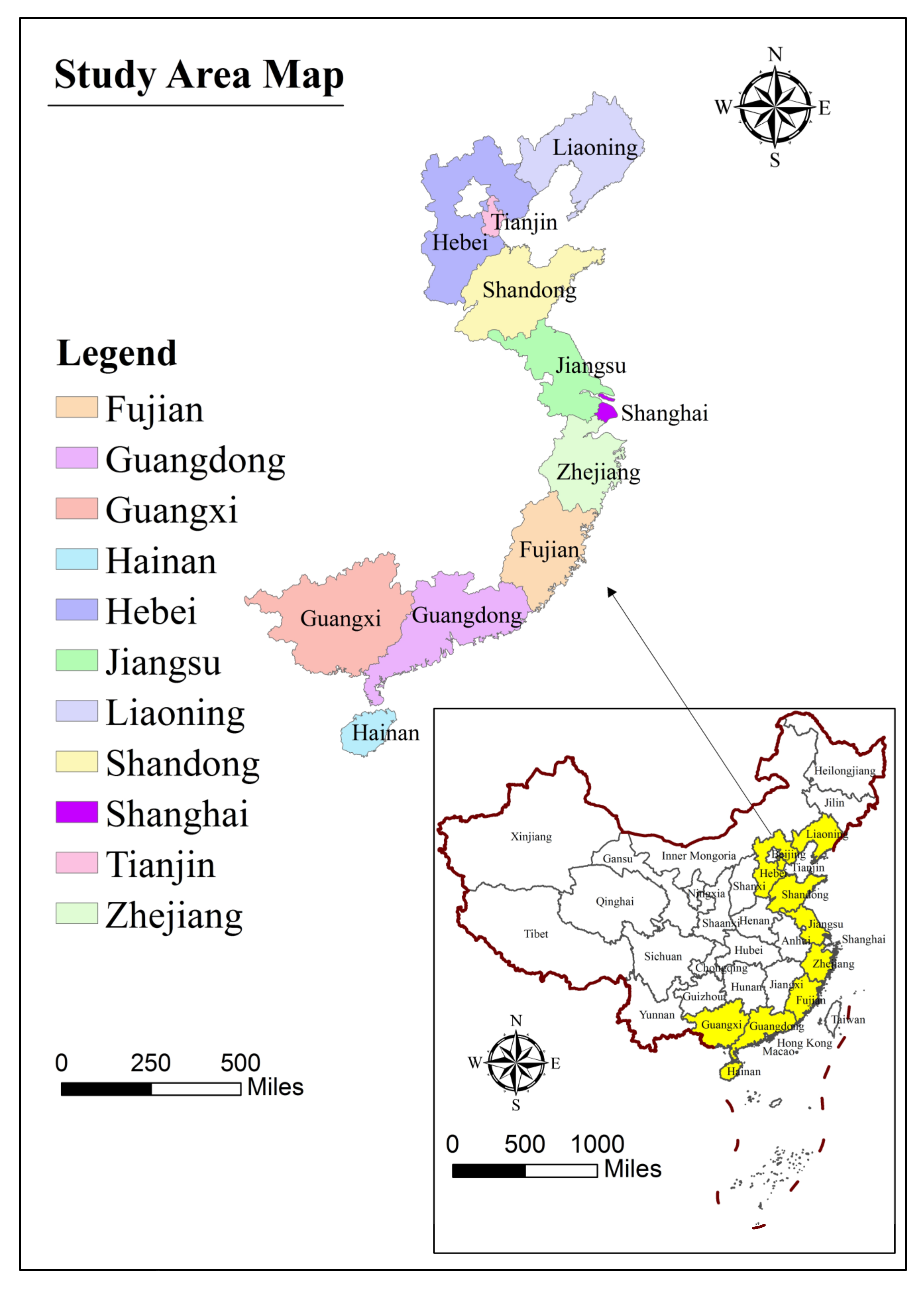
The paper analyzed the panel data of 11 provinces along China’s coast from 2006 to 2018 (Figure 2). The data are mainly from the 2007–2019 China Marine Statistics Yearbook, the China Statistical Yearbook, and the China Environmental Statistics Yearbook. The missing data are supplemented by the interpolation method. Considering the resource and environmental constraints in the marine economic system, this paper incorporated the utilization of marine resources and their impact on the environment into the evaluation system based on capital and labor inputs.

The specific indicators are as follows:

2.3.1. Input Indicator

(1) Capital.

In this paper, the marine economic capital stock was used as the capital input index. The capital stock measures the total cost of construction and acquisition of fixed assets related to production activities over a period. Referring to the research of Shan [39], this paper used the perpetual inventory method to measure the fixed assets of 11 coastal areas. As shown in Formula (10):

$$K_{i,t}=I_{i,t}/P_{i,t}+\left(1-{\delta }_{i,t}\right)K_{i,t-1}$$

(10)

$K_{i,t}$ and $K_{i,t-1}$ represent the capital stock in period $t$ and $t_1$ respectively, $I_{i,t}$ indicates the investment for the current year, expressed in terms of fixed asset completions, and $P_{i,t}$ represents the fixed asset investment price index for each province for the year. This paper selected 2006 as the base period and drew on Xu’s treatment method [40] to determine the capital stock of the base period in each region as: $K_{i,2006}=I_{i,2006}/({\delta }_{2006}+g_{iy})$, and $g_{iy}$ to the average annual growth rate of the $i$ region for 2006–2018. ${\delta }_{i,t}$ represents the depreciation rate of the total amount of fixed asset formation. Drawing on the practice of Shan [39], ${\delta }_{i,t}$ takes the value of 10.96%. Finally, the capital stock data of coastal provinces were converted into marine economic capital stock by reference to the research of He et al. [41]. The formula is as follows:

$$K_{i{t}_m}=K_{it}\times \frac{Y_{i{t}_m}}{Y_{it}}$$

(11)

Among them, $Y_{it}$, $K_{it}$, $Y_{i{t}_m}$, and $K_{i{t}_m}$ represent the gross domestic product (GDP), capital stock, GOP, and marine capital stock of coastal provinces, respectively.

(2) Labor.

In the Marine Economic Statistics Yearbook, after 2006, the number of sea-related employees in coastal areas was used to reflect the amount of labor input, which has been used until now, and the data is comparable. Therefore, with reference to the results of national economic research, the paper selected this indicator to measure labor input and records it as L.

(3) Resource.

Because the development of the marine economy is highly dependent on resource endowment, the input of marine resources is very important to the development of marine economy. Drawing on the practice of Zhao et al. [42], this paper selected the length of the wharf, the number of coastal travel agencies, and the area of marine aquaculture. It was then converted using the entropy method as a comprehensive indicator of resource input. The calculation process for the composite indicators is as follows:

• Non-quantitative processing of indicators. The original indicator data matrix is $X_{ij}={\left(x_{ij}\right)}_{m\times n}$, wherein the $X_{ij}$ is the value of the regional i indicator j, the proportion of this value is $X_{ij}=X_{ij}/\sum _{i=1}^m{X}_{ij}$. Therefore, the original matrix can be converted into a scaleless matrix $X_{ij}^{\prime }={\left(x_{ij}^{\prime }\right)}_{m\times n}$.
• Calculate the entropy value $e_j$ of indicator j:$e_j=-\frac{1}{ln m}\sum _{i=1}^m{X}_{ij}^{\prime }ln{x}_{ij},e_j\ge 0$.
• Calculate the difference coefficient $e_j^{\prime }$ of indicator $j$. Given the indicator $j$, the smaller the difference between the $X_{ij}^{\prime }$ of each sample, the greater the entropy value $e_j^{\prime }$, the smaller the role of indicator $j$ in the comprehensive evaluation. We define $e_j^{\prime }=1-e_j$, So, the bigger the $e_j^{\prime }$, the more important the indicator $j$ is in the comprehensive evaluation.
• Calculate the objective weight of indicator j:$w_j=e_j^{\prime }/{\sum }_{j=1}^n{e}_j=\left(1-e_j\right)/\sum _{j=1}^n\left(1-e_j\right)$.
• Calculate the composite index of resource inputs h:$h=\sum _{j=1}^n{X}_{ij}^{\prime }{w}_j$.

Through the above measurement steps, the weights of the length of the wharf, the number of coastal travel agencies and the area of marine aquaculture in 2006–2018 were 0.219, 0.167, and 0.614 respectively, and the resource input index was obtained as the final value according to the comprehensive weighting of this weight.

2.3.2. Output Indicator

(1) Desirable output.

The economic benefits brought by marine resources can well reflect the development of the marine economy [43,44]. Therefore, the GOP was used as the desirable output of the model. The regional GOP was converted to constant price levels on a 2006 basis [45].

(2) Undesirable output.

Marine economy is similar to the national economy, in that the production and operation process will also have a negative impact on the ecological environment. Therefore, based on taking full account of the particularity and data accessibility of the marine economy, we followed the practice of Zang [46] and used the research results of Zeng [47] to select marine wastewater, marine exhaust gas, and marine solid waste emissions as environmental pollution indicators.

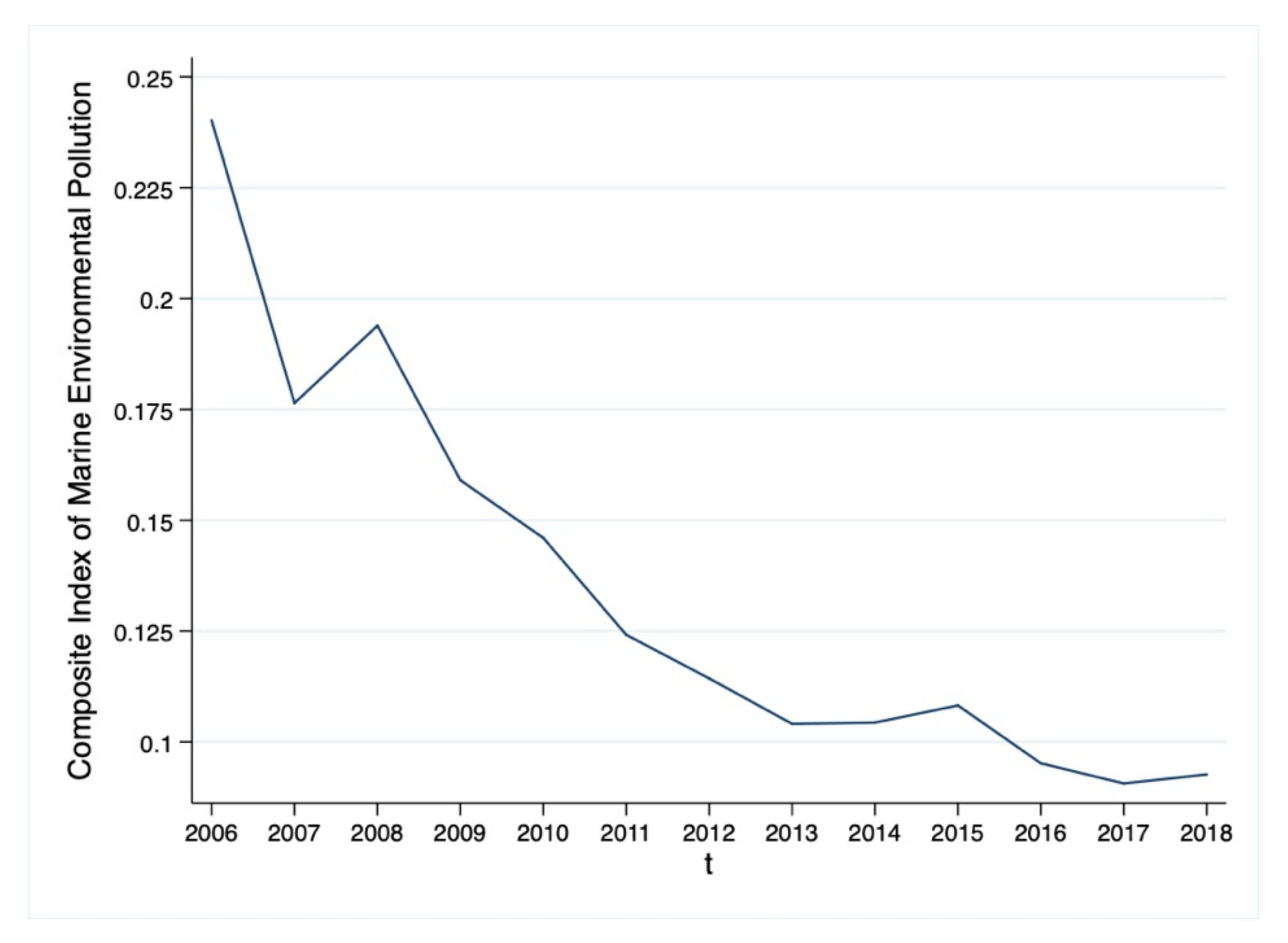
Marine industrial pollution emissions were converted according to “(GOP/GDP) × industry pollution emissions”. 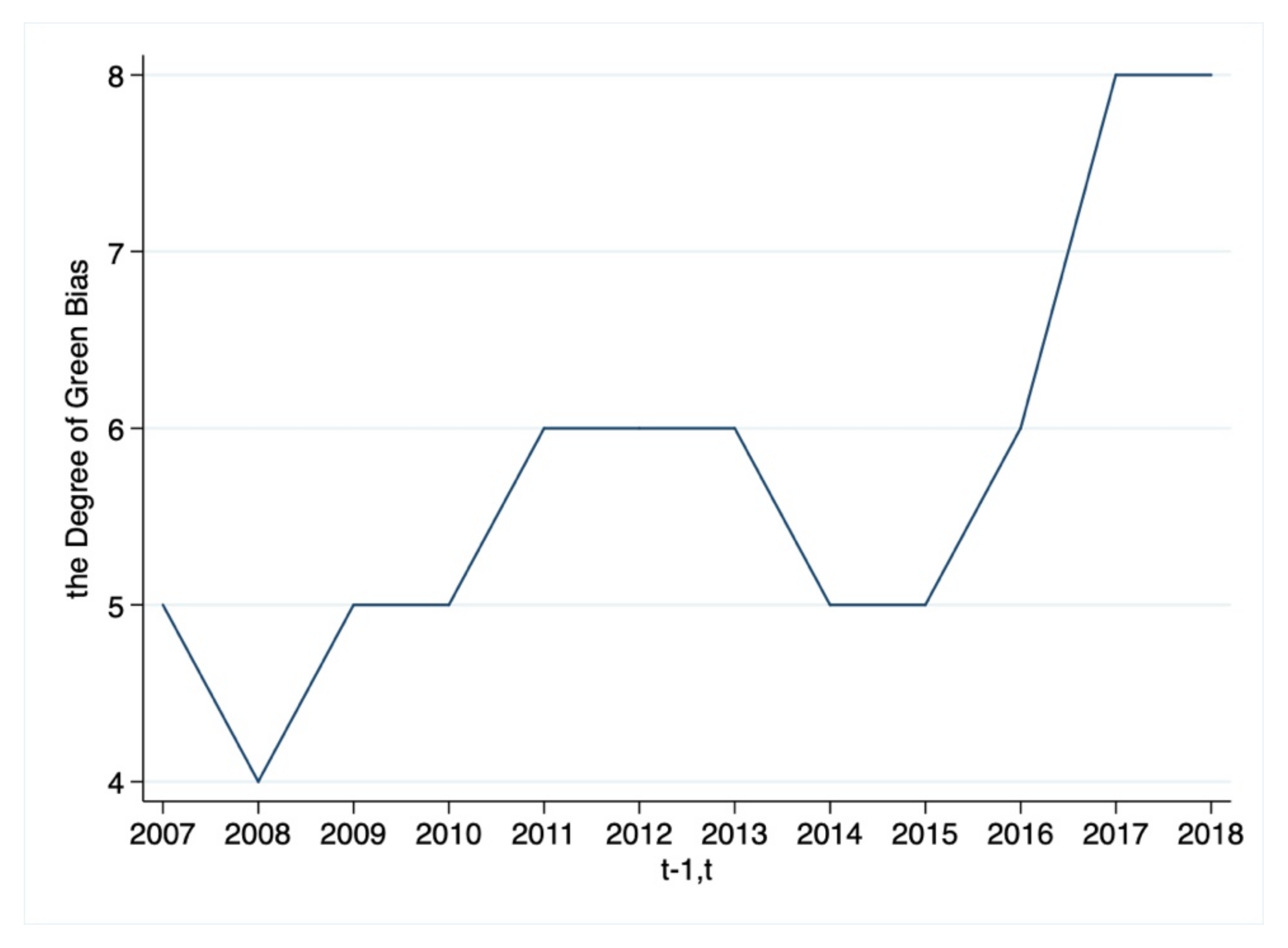Then, using the entropy method, the weights of total marine wastewater discharge, total exhaust emission, and solid waste emission were 0.150, 0.127, and 0.723 respectively, according to which the three indicators of marine “three waste” emissions were combined into a comprehensive index of marine environmental pollution $H$ [48]. This was used as an indicator of undesirable outputs. The larger the indicator, the more serious the pollution of the marine environment. China’s coastal environmental pollution index is shown in Figure 3:

As can be seen from Figure 3, the pollution index $H$ in 2006–2018 shows a small range of fluctuations and an overall downward trend. Specifically, before 2008, the fluctuation of marine environmental pollution index in coastal areas of China was relatively obvious. At this stage, the marine economy has been constantly subjected to structural adjustment, the development of which is relatively extensive. Between 2008 and 2013, the comprehensive index $H$ began to decline year by year. This is mainly due to the formulation and implementation of the government’s policies on the regulation of the marine environment, as well as the continuous promotion of marine environmental protection. After 2013, the pollution index $H$ showed a steady downward trend, which was due to the implementation of policies, a positive effect of the previous policy on the environment that was highlighted. The development of marine green production technology has made the marine environmental protection stable and progressive during this period.

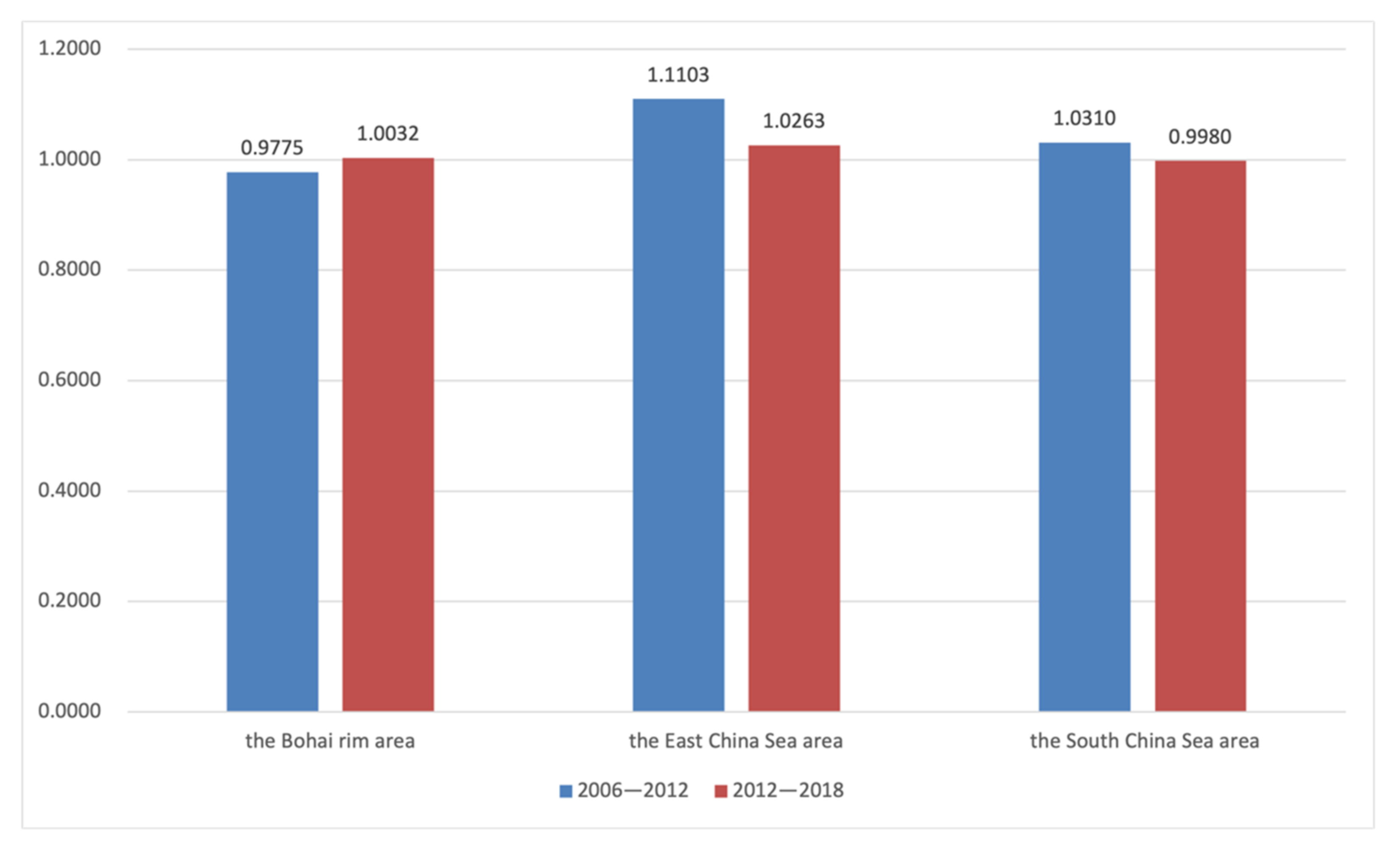
Combining the above factors, the GTFP was measured. Referring to the Classification and Code of Coastal Administrative Areas (HY/T094-2006), the 11 coastal provinces are divided into the areas of Bohai rim, the East China Sea, and the South China Sea. Among them, the Bohai rim area includes Tianjin, Hebei, Liaoning, and Shandong. The area of East China Sea includes Shanghai, Jiangsu, and Zhejiang. The area of South China Sea includes Fujian, Guangdong, Guangxi, and Hainan.

Table 2. Descriptive statistics for the main indicators.

Indicator	Variable	Units	Mean	Std. Dev	Median	Min	Max	Number of Samples
Desirable output	GOP	RMB 100 million	3644.188	232.584	2936.054	300.700	12,026.370	143
Resource input	Number of travel agencies in coastal areas		1141.350	54.585	1116	147	2872	143
	Pier length	m	57,312.350	3496.883	48426	5355	176,208	143
	Area of use in the sea	hectares	23,634.275	3038.834	6150	12.800	173,633.800	143
Labor input	Number of people involved in the sea	ten thousand	309.9302	17.8635	209.8000	81.5000	900.5944	143
Capital investment	Marine capital stock	RMB 100 million	9480.742	613.359	8297.697	475.508	35,703.378	143
Undesirable output	Marine wastewater	tons	16,263.927	945.964	13,075.339	1090.931	43,807.600	143
	Marine exhaust gas	100 million cubic meters	3764.741	211.642	3639.371	254.560	14,402.058	143
	Marine solid waste	tons	0.359	0.069	0.019	0	5.232	143

gives the basic characteristics of the input and output indicator data. The ratio of the maximum and minimum capital input is 75.08, and the mean value of capital input exceeds the median; the ratio of maximum to minimum labor input is about 11.05, which is the smallest of several other inputs, and the standard deviation and median of the three resource input indicators are very different. It can be seen that the difference between provinces in capital input is large, material capital input shows path dependence, and the capital stock of large provinces have absorbed and accumulated more capital, resulting in the phenomenon of factor aggregation; in recent years, the mobility of the labor force between provinces is large, the distribution of labor input between provinces is relatively small, but there is still a certain gap between the quality and skill level of the labor force in different provinces; the marine economic development of each province is highly dependent on resources, but the distribution is more scattered. From the output point of view, the maximum desirable output is close to 40 times the minimum value, the scale and speed of inter-provincial marine economic growth are very different, and the maximum desirable output is also dozens of times the minimum, reflecting that the marine economic development of many provinces is at the expense of the environment, and China’s marine environmental efficiency still needs to be improved.

3. Results

3.1. Dynamic Evolution of GTFP and Decomposition Components

Based on input and output data for China’s coastal areas from 2006 to 2018, the ML index, reflecting the changes of GTFP in each province, was calculated by MAXDEA software, and the ML index was broken down into the TC index and EC index. The trend over the same period for each index is shown in Figure 4. It is not difficult to see that the overall ocean GTFP is in a state of steady growth. The TC index is more in line with the ML index for each year, while the EC index is close to one in most years, indicating that technological progress in marine development has a stable effect on the growth of ocean GTFP, while the change of technical efficiency has no significant effect on GTFP.

The TC index can be further broken down into IBTC, OBTC, and MATC indices. The MATC index is less than the TC index in each year, indicating that the efficiency of the technology scale has not played a positive role in technological progress, possibly because the imbalance of the development of marine industry limits the efficiency of the technology scale. When compared with the IBTC index, the curve trend of the OBTC index is highly compatible with the TC curve, indicating that technological progress is not neutral, and that output bias is closely related to the change of technological progress.

Figure 5 shows more clearly the movement of the OBTC index and the ML index over the same period. The OBTC index and the ML index have a certain consistency of the trend of change, indicating that the output-biased technological progress has a significant impact on the ocean GTFP. The two indices fluctuated significantly between 2008 and 2012. However, 2012 was a turning point, since after a short period of small fluctuations, the two indices improved after 2013 and the volatility trend was more stable. From the perspective of the size of the index, there is still a lot of room for progress in the adaptive and technological diffusion of China’s marine economic development.

3.2. Regional Distribution of the Marine Green OBTC Index

Figure 6 reflects the OBTC index and trends in the three regions around 2012. It can be seen that after 2012, the OBTC index of the Bohai rim area had increased, while the OBTC index of the East China Sea area and the South China Sea area had decreased slightly, but the value of the OBTC Index in most regions is greater than one, which shows that the closely introduced marine environmental protection policy effectively corrects the negative externalities of marine production, constrains the relevant practitioners to carry out green production, technological innovation, and industrial restructuring, and forms a win–win situation of ecological and economic common development. Among them, the OBTC index of the East China Sea area is higher than that of the Bohai rim area and the South China Sea area. It is basically in line with the current situation of marine economic development in various regions. In contrast, the OBTC index in the South China Sea area is the lowest.

Table 3. ML and OBTC indices for each province.

Region	Province	ML	OBTC
Bohai rim area	Tianjin	1.0802	1.0156
	Hebei	0.9940	1.0076
	Liaoning	1.0513	1.0020
	Shandong	0.9368	0.9364
East China Sea area	Shanghai	1.1943	1.2017
	Jiangsu	1.0106	1.0025
	Zhejiang	1.0085	1.0006
South China Sea area	Fujian	1.0030	1.0044
	Guangdong	0.9871	1.0105
	Guangxi	0.9803	1.0086
	Hainan	0.9948	1.0345
Average for coastal areas		1.0219	1.02039

shows the cumulative changes in the Marine Economic ML index and OBTC index in different coastal provinces of China from 2006 to 2018, represented by their respective averages. During the sample period, the ML and OBTC indices were consistently between [0.9368, 1.2017] and were generally stable. On average, in coastal areas, the ML and OBTC indices grew steadily at 2.19% and 2.04%, respectively, reflecting the fact that the output bias of current technological progress has overall supported the growth of the marine economy. Six of the nine provinces have an ML index greater than one, indicating that the ocean GTFP is on the rise in most areas.

Judging from the index vibration range, the imbalance in the development of the regional marine economy is significant. The Shandong ML and OBTC indices fell the most, by an average of about 6.32 and 6.36% per year, indicating that the OBTC in Shandong has not played a significant economic promotion role. In addition, Hebei, Guangdong, Guangxi, and Hainan also saw small declines. However, the ML and OBTC indices in Shanghai rose the most. They grew at a rate of about 19.43 and 20.17% per year, respectively. Both are at the highest level in the coastal areas. This was followed by Tianjin and Liaoning. In addition, Jiangsu, Zhejiang, and Fujian provinces have seen small increases, indicating that these provinces can still achieve efficient green marine growth through rational adjustment of pollution control, while achieving a steady annual growth rate of 5.8%. From these data, it is also sufficient to see that the OBTC and GTFP changes have a certain consistency.

3.3. Analysis of Specific Output Biases for Technological Progress

The measurement of the OBTC index reflects the existence of output-biased technological progress, and whether the OBTC index has contributed to the growth of GTFP. Next, this paper further analyzed the rationality of the existing bias, that is, to determine whether China’s marine technology is biased towards reducing marine environmental pollution and whether marine development conforms to the concept of green environmental protection. Based on the output bias judgment method proposed in Section 2.2.4, we calculated the intertemporal ratio of the expected output indicator to the undesirable output indicator. Next, we combined it with the OBTC index to identify the output bias of marine technology progress in each province, in each year, and analyzed its change law.

Figure 7 shows the trend in the number of provinces where marine technology is biased towards reducing marine waste in 2006–2018, which reflects the degree of green bias in marine economic development over the years. During the study period, the number of provinces whose marine output was biased towards reducing pollutant emissions increased. Around 2008 and 2013, the degree of green bias in marine economic development was under market and policy pressures, respectively. The former was negatively affected by the macro economic crisis, while the latter was due to 2012 as an inflection point, and the Report stressed the construction policy of the maritime power strategy in a short period of time after the implementation of the policy to balance the use of resources and the ecological environment protections, hence the marine environment appears as short-term fluctuations. Since then, however, the degree of marine green bias has increased significantly since 2014, reflecting the vulnerability and sensitivity of the marine environment.

Table 4. Output bias over time.

Year	OBTC	$\mathbf{M}\mathbf{R}{\mathbf{T}}_{\mathbf{b}\mathbf{g}}$	Bias
2006–2007	1.0741	0.8088	$Y_b$
2007–2008	1.0515	0.8596	$Y_b$
2008–2009	1.0069	0.8915	$Y_b$
2009–2010	1.1178	0.8625	$Y_b$
2010–2011	0.9491	0.9901	$Y_g$
2011–2012	0.9994	0.8627	$Y_g$
2012–2013	0.9900	0.9098	$Y_g$
2013–2014	1.0038	0.8976	$Y_b$
2014–2015	1.0525	0.9517	$Y_b$
2015–2016	1.0047	0.7971	$Y_b$
2016–2017	1.0370	0.9708	$Y_b$
2017–2018	0.9578	0.9659	$Y_g$

shows changes in output bias for 2006–2018. As can be seen, 8 of the 12 time periods were biased towards increased marine pollution and only four were biased towards increased desirable output.

Table 5. Regional output bias.

	2006–2009			2009–2012			2012–2015			2015–2018
	OBTC	$\mathbf{M}\mathbf{R}{\mathbf{T}}_{\mathbf{b}\mathbf{g}}$	Bias	OBTC	$\mathbf{M}\mathbf{R}{\mathbf{T}}_{\mathbf{b}\mathbf{g}}$	Bias	OBTC	$\mathbf{M}\mathbf{R}{\mathbf{T}}_{\mathbf{b}\mathbf{g}}$	Bias	OBTC	$\mathbf{M}\mathbf{R}{\mathbf{T}}_{\mathbf{b}\mathbf{g}}$	Bias
Tianjin	1.0059	0.8079	$Y_b$	1.0267	0.9885	$Y_b$	1.0081	0.9020	$Y_b$	1.0215	0.9855	$Y_b$
Hebei	1.0091	0.8143	$Y_b$	1.0212	0.6070	$Y_b$	1.0002	0.9857	$Y_b$	1.0001	0.9313	$Y_b$
Liaoning	0.9964	0.5983	$Y_g$	1.0113	1.2654	$Y_g$	1.0002	0.9415	$Y_b$	0.9999	0.6181	$Y_g$
Shanghai	1.2971	0.7471	$Y_b$	1.3588	1.0597	$Y_g$	1.1916	0.8679	$Y_b$	0.9592	0.8785	$Y_g$
Jiangsu	1.0032	0.9603	$Y_b$	1.0032	0.9651	$Y_b$	1.0094	0.9153	$Y_b$	0.9941	0.8435	$Y_g$
Zhejiang	0.9974	0.8553	$Y_g$	1.0018	0.8672	$Y_b$	1.0034	0.8726	$Y_b$	0.9999	0.8799	$Y_g$
Fujian	1.0002	0.9090	$Y_b$	1.0054	0.7197	$Y_b$	1.0102	0.9334	$Y_b$	1.0016	1.1875	$Y_g$
Shandong	1.0150	0.9765	$Y_b$	0.7346	0.9567	$Y_g$	0.9963	0.9869	$Y_g$	0.9996	0.9253	$Y_g$
Guangdong	1.0791	0.9579	$Y_b$	0.9958	0.7444	$Y_g$	0.9767	0.8687	$Y_g$	0.9903	0.9065	$Y_g$
Guangxi	1.0000	0.7819	$Y_g$	1.0073	0.6040	$Y_b$	1.0001	0.8048	$Y_b$	1.0270	0.8642	$Y_b$
Hainan	1.0829	0.9775	$Y_b$	1.0771	1.1786	$Y_g$	0.9733	1.0380	$Y_b$	1.0046	1.0039	$Y_g$
All	1.0442	0.8533	$Y_b$	1.0221	0.9051	$Y_b$	1.0154	0.9197	$Y_b$	0.9998	0.9113	$Y_g$

provides a visual indication of the bias of output-biased technological progress in different regions towards different outputs, with data showing the average of the indices divided over a three-year period in each coastal province. It can be seen from the data comparison that overall output-biased technological progress tends to increase environmental pollution rather than increase desirable output. However, there has been a marked increase in green bias nationwide in 2015–2018, which is consistent with the time trend characteristics of output bias. Specific to the provinces, it can be found that in recent years, Liaoning, Shanghai, Jiangsu, Zhejiang, Fujian, Shandong, Guangdong, and Hainan have paid more attention to the improvement of the quality of the marine environment. In contrast, Tianjin, Hebei, and Guangxi have been more inclined to increase total factor productivity and boost marine economic growth by emitting more pollutants. From the perspective of time, the output bias after 2012 is driven in the direction of $Y_g$.

Table 6. Percentage of provinces in different regions where technological progress tends to the reduction of undesirable output over time.

Region	Percentage of Provinces in Each Region over the Period Where OBTC Tend to Reduce Pollutant Emissions (%)
	2006–2018	2006–2012	2012–2018
Bohai rim area	41.67	37.5	45.83
East China Sea area	63.88	61.11	66.67
South China Sea area	54.17	45.83	62.5

shows the proportion of provinces in various regions that have been biased towards reducing marine pollutant emissions as a percentage of the total number of provinces in the region. Between 2006 and 2018, technological progress in most provinces of the East China Sea area and the South China Sea area tended to reduce pollutant emissions, while the Bohai rim area tended to increase the total output value. After 2012, the degree of green bias in various regions has improved significantly.

Specifically, the green bias of the marine economy in the East China Sea area is the highest, and the OBTC index is also the highest. In contrast, the green bias degree and OBTC index of the Bohai rim area are the lowest, but in recent years, its ML index, OBTC index, and green bias degree rose step by step. However, the area of South China Sea’s green bias increased significantly in 2012–2018, while its OBTC index declined during that period.

4. Discussion

4.1. Analysis of the Existence and Trend of Output-Biased Technological Progress

From the dynamic evolution and regional differences of the OBTC index, there is obvious output-biased technological progress in the development process of China’s marine economy, and its change trend is highly consistent with GTFP, indicating that the changes between the two have a strong correlation.

As far as the time change of OBTC index is concerned, 2008 was negatively affected by the macro economy, resulting in a decline in the efficiency of the marine economy, and in the early stage of the development of the marine economy, resource constraints and environmental pollution also caused a certain degree of efficiency loss. However, in the Report of 2012, the requirements for marine ecological protection were clearly emphasized, and since then, the national governments at all levels have formulated corresponding policies in response to the national strategy, but the marine economic development has a certain period of adaptation to the implementation of the policy. Subsequently, the two indices stabilized, reflecting that the marine macro policy can improve the marine environment and stabilize the marine economic development.

From the perspective of the regional differences of the OBTC index, the index is from high to low in the East China Sea, the Bohai rim, and the South China Sea area. The reason for this is that the East China Sea area has sufficient funds and human resources into marine science and technology and production, which is conducive to the improvement of the marine economy. As far as the area of South China Sea is concerned, although the marine economy of Guangdong and Fujian is relatively developed, the marine economy of Guangxi and Hainan is not very good. Without sufficient funds and human resources, the innovation capacity of marine science and technology is relatively low, and the effectiveness of marine economic technology is low.

Specifically, from each province, the impact of the OBTC index on the development of the marine economy varies from region to region. Among them, the higher indices of Shanghai are related to its strong capital and higher-level talent pool, while the decline of Shandong’s indices are large. Perhaps, due to the diminishing marginal return of marine scientific and technological output and the low effective conversion rate of related achievements, the promotion effect on GTFP is not fully reflected.

4.2. The Role of Technological Progress in Promoting the Bias of Green Output

Judging from the time fluctuation trend of green output bias, in the process of reducing marine pollution, there is constant pressure from the production model of sacrificing the environment in exchange for the increase in marine GDP, but the marine environmental protection policies generally guarantee the green development of the ocean. When combining it with the output bias of Table 4, although the degree of marine green bias has increased significantly in recent years, the marine environmental protection in the coastal provinces is still relatively weak, and the overall trend is still biased towards more extensive growth.

From the perspective of regional differences, the degree of green output bias of technological progress in coastal provinces is obviously different. Among them, Guangxi’s OBTC and ${\mathrm{MRT}}_{\mathrm{bg}}$ indices have a large gap in each period, which is because Guangxi has undertaken many industrial transfers, with serious pollution and high emissions. The low level of marine industrial structure, the high energy consumption of economic output, and the extensive development mode [49] have led to a weak foundation of the province and a lower marine economic output value than the national average, which ultimately aggravates the contradiction between Guangxi’s marine economic development and the improvement of marine environmental quality.

When combining the dynamic data of different periods with the realistic background, the 2012 Report put forward new requirements for marine economic development, and local governments have formulated corresponding policies in response to national strategies. Since the formulation and implementation of policies often have a certain lag [50], after a short-term policy adjustment, in recent years, as well as the continuous progress, diffusion and innovation of modern technological levels, the marine economy has developed in the direction of increasing the desired output and reducing pollution emissions, and the national marine environmental governance policy has achieved results.

Judging from the changes in the proportion of provinces in various areas to reduce pollutant emissions, China’s coastal areas have achieved certain results in rationally utilizing marine resources and controlling pollution emissions. Overall, however, there is still much room for improvement in the number of provinces in various regions that are biased towards protecting the environment. Among them, the degree of green output bias from high to low is the East China Sea, the South China Sea, and the Bohai rim area, but the Bohai rim area has risen significantly in recent years. It shows that the East China Sea region has effectively coordinated the relationship between the growth of marine economic output value and environmental protection, while the coordination of the two in the South China Sea region needs to be strengthened. However, in the early stage of the development of the marine economy, the Bohai rim area has paid too much attention to the improvement of the total marine output value and ignored the protection of the marine environment, but the increase in their green bias of its output in the later period gradually played a leading role in its economic growth, and the overall environmental protection measures in the region still need to be further strengthened.

In summary, this paper discusses the dynamic link between technological progress and the bias of green output in China’s marine economy. In the follow-up study, we will further conduct a detailed quantitative analysis of the degree of green bias, and analyze the factors that affect the green output bias of marine technology progress, to make more targeted suggestions for the green development of the marine economy.

5. Conclusions

The novelty of this study is that the green development of the marine economy was discussed from the perspective of output, and the OBTC index of each region in each year was calculated to determine whether there is a significant output-biased technological progress in the development of China’s marine economy. Furthermore, we studied the rationality of the current output-biased technological progress, intuitively reflected the differences in the degree of green bias in coastal areas, and discussed whether technological progress has promoted the green output bias of the marine economy, that is, to determine whether China’s marine economy has developed in the direction of increasing the desirable output and reducing the undesirable output.

The results show that there is obvious output-biased technological progress in China’s marine economy, and this output-biased technological progress has led to the improvement of GTFP. During the sample period, although most of China’s coastal areas in general still tend to pursue the improvement of the total output value of the marine economy at the expense of the environment, the green bias has improved significantly after 2015, driven by the active policies of the relevant marine environment protection. It shows that technological progress has increased the bias of green output in the marine economy. From the perspective of different areas, the imbalance in the development of the regional marine economy is significant. The East China Sea area has the highest green bias, while the Bohai rim area has the lowest. However, the coordination between the development of the green marine economy and environmental protection in the South China Sea area needs to be improved.

To achieve sustainable development of the marine economy, coastal areas should control undesirable output as much as possible. Overall, all regions should try to avoid the negative externalities caused by environmental pollution and improve the level of green output. In view of the different areas, relevant departments should formulate differentiated management policies according to the specific situation in each region. Among them, we should pay attention to the environmental protection of the Bohai rim area, the comprehensive strength of green marine development in the South China Sea area, and the efficiency of green marine output in the East China Sea area. In this way, it will promote the coordinated development of the interregional marine economy.

References

1. Chen, J.; Wang, Y.; Song, M.; Zhao, R. Analyzing the decoupling relationship between marine economic growth and marine pollution in China. Ocean Eng. 2017, 137, 1–12. [Google Scholar] [CrossRef]
2. Jiang, X.Z.; Liu, T.Y.; Su, C.W. China’s marine economy and regional development. Mar. Policy 2014, 50, 227–237. [Google Scholar] [CrossRef]
3. Ji, J.Y.; Sun, X.W. Research on connotation and evaluation framework of the transformation and upgrading of marine industry. J. Ocean. Univ. China (Soc. Sci.) 2021, 11, 33–40. [Google Scholar] [CrossRef]
4. Yuan, Q.M.; Zhang, W.L.; Feng, D. An analysis of Chinese marine economic efficiency change and productivity change under constraints of resources and environment. Econ. Surv. 2016, 33, 13–18. [Google Scholar] [CrossRef]
5. Wang, S.H.; Sun, X.L.; Song, M.L. Environmental regulation, resource misallocation, and ecological efficiency. Emerg. Mark. Financ. Trade 2021, 57, 611–630. [Google Scholar] [CrossRef]
6. Wang, S.H.; Wang, X.Q.; Lu, B.B. Is Resource Abundance a Curse for Green Economic Growth? Evidence from Developing Countries. Resour. Policy 2021, 75, 102533. [Google Scholar] [CrossRef]
7. Wang, B.H.; Zhang, X. Measurement and analysis of industrial biased technological progress in China based on SBM directional distance function. Sci. Technol. Manag. Res. 2021, 13, 107–116. [Google Scholar] [CrossRef]
8. Zhang, X.H.; Wu, L.L.; Shi, P.; Li, N.; Liu, X.F. Research on the countermeasures of green development of “Blue Economy” in Guangdong-Hong Kong-Macao greater bay area. Ecol. Econ. 2021, 37, 59–63. [Google Scholar]
9. Wang, S.H.; Chen, S.S.; Zhang, H.Y.; Song, M.L. The Model of Early Warning for China’s Marine Ecology-Economy Symbiosis Security. Mar. Policy 2021, 128, 104476. [Google Scholar] [CrossRef]
10. Ding, L.L.; Zhu, L.; He, G.S. Measurement and influencing factors of green total factor productivity of marine economy in China. Forum Sci. Technol. China 2015, 2, 72–78. [Google Scholar] [CrossRef]
11. Wang, S.H.; Lu, B.B.; Yin, K.D. Financial development, productivity, and high-quality development of the marine economy. Mar. Policy 2021, 130, 104553. [Google Scholar] [CrossRef]
12. Soug, M.; Wang, S. Measuring environment-biased technological progress considering energy saving and emission reduction. Process Saf. Environ. Prot. 2018, 116, 745–753. [Google Scholar] [CrossRef]
13. Zha, D.; Kavuri, A.S.; Si, S. Energy-biased technical change in the Chinese industrial sector with CES production functions. Energy 2018, 148, 896–903. [Google Scholar] [CrossRef] [Green Version]
14. Wang, S.H.; Chen, M.; Song, M.L. Energy constraints, green technological progress, and business profit ratios: Evidence from big data of Chinese enterprises. Int. J. Prod. Res. 2018, 56, 2963–2974. [Google Scholar] [CrossRef]
15. Khalid, B.; Naumova, E. Digital transformation SCM in view of Covid-19 from Thailand SMEs perspective. In Global Challenges of Digital Transformation of Markets; Nova Science Publishers, Inc.: New York, NY, USA, 2021; pp. 49–66. [Google Scholar]
16. Barykin, S.Y.; Kapustina, I.V.; Sergeev, S.M.; Kalinina, O.V.; Vilken, V.V.; de la Poza, E.; Putikhin, Y.Y.; Volkova, L.V. Developing the physical distribution digital twin model within the trade network. Acad. Strateg. Manag. J. 2021, 20, 1–18. [Google Scholar]
17. Zhang, C.; Quan, Y.; Zhong, H. The building of marine ecological civilization and sustainable development: Conference report. Mar. Policy 2019, 110, 103627. [Google Scholar] [CrossRef]
18. Unger, S.; Müller, A.; Rochette, J.; Schmidt, S.; Shackeroff, J.; Wright, G. Achieving the Sustainable Development Goal for the Oceans; IASS Policy Brief; Institute for Advanced Sustainability Studies: Potsdam, Germany, 2017; Volume 1. [Google Scholar] [CrossRef]
19. Wang, L.; Zhang, H. The impact of marine tourism resources development on sustainable development of marine economy. J. Coast. Res. 2019, 94, 589–592. [Google Scholar] [CrossRef]
20. Suris-Regueiro, J.C.; Garza-Gil, M.D.; Varela-Lafuente, M.M. Marine economy: A proposal for its definition in the European Union. Mar. Econ. 2013, 42, 111–124. [Google Scholar] [CrossRef]
21. Morrissey, K.; O’Donoghue, C. The Irish marine economy and regional development. Mar. Policy 2012, 36, 358–364. [Google Scholar] [CrossRef]
22. Stebbings, E.; Papathanasopoulou, E.; Hooper, T.; Austen, M.C.; Yan, X.Y. The marine economy of the United Kingdom. Mar. Policy 2020, 116, 103905. [Google Scholar] [CrossRef]
23. Sun, C.Z.; Li, M.Y. Spatial-Temporal change of coastline in Liaoning province and its driving factor analysis. Geogr. Geo-Inf. Sci. 2010, 3, 63–67. [Google Scholar]
24. Antonell, C. Technological congruence and the economic complexity of technological change. Struct. Chang. Econ. Dyn. 2016, 38, 15–24. [Google Scholar] [CrossRef]
25. Feder, C. The effects of disruptive innovations on productivity. Technol. Forecast. Soc. 2018, 126, 186–193. [Google Scholar] [CrossRef]
26. Briec, W.; Peypoch, N. Biased technical change and parallel neutrality. J. Econ. 2007, 92, 281–292. [Google Scholar] [CrossRef]
27. Chen, P.C.; Yu, M.M. Total factor productivity growth and directions of technical change bias: Evidence from 99 OECD and nonOECD countries. Ann. Oper. Res. 2014, 214, 143–165. [Google Scholar] [CrossRef]
28. Zheng, H.; Zhang, J.C.; Zhao, X.; Mu, H.R. Exploring the affecting mechanism between environmental regulation and economic efficiency: New evidence from China′s coastal areas. Ocean Coast. Manag. 2020, 189, 105–114. [Google Scholar] [CrossRef]
29. Yu, M.M.; Hsu, C.C. Service productivity and biased technological change of domestic airports in Taiwan. Int. J. Sustain. Transp. 2012, 6, 1–25. [Google Scholar] [CrossRef]
30. Mizobuchi, H. Multiple Directions for Measuring Biased Technical Change; University of Queensland Press: Brisbane, Australia, 2015. [Google Scholar]
31. Hampf, B.; Kruger, J.J. Estimating the bias in technical change: A nonparametric approach. Econ. Lett. 2017, 157, 88–91. [Google Scholar] [CrossRef]
32. Di, Q.B.; Zhao, X.M.; Wang, M. Ecological efficiency evaluation of China coastal tourism based on undesired output: China coastal city case. Mar. Sci. Bull. 2020, 39, 160–168. [Google Scholar] [CrossRef]
33. Fare, R.; Grifell-Tatjé, E.; Grosskopf, S.; Knox Lovell, C.A. Biased Technical Change and the Malmquist Productivity Index. Scand. J. Econ. 1997, 99, 119–127. [Google Scholar] [CrossRef]
34. Weber, W.L.; Domazlicky, B.R. Total factor productivity growth in manufacturing: A regional approach using linear programming. Reg. Sci. Urban. Econ. 1999, 29, 105–122. [Google Scholar] [CrossRef]
35. Portela, M.C.A.S.; Thanassoulis, E.; Simpson, G. Negative data in DEA: A directional distance approach applied to bank branches. J. Oper. Res. Soc. 2004, 55, 1111–1121. [Google Scholar] [CrossRef] [Green Version]
36. Chen, L.M.; Wang, W.P.; Wang, B. Environmental regulation-induced environmental technological innovation and its bias. J. Ind. Eng. Eng. Manag. 2018, 32, 186–195. [Google Scholar] [CrossRef]
37. Chung, Y.H.; Fare, R.; Grosskopf, S. Productivity and undesirable outputs: A directional distance function approach. J. Environ. Manag. 1997, 51, 229–240. [Google Scholar] [CrossRef] [Green Version]
38. Li, J.; Chi, J.; Wu, H.Q. Measurement and analysis of industrial green biased technological progress based on water resources. China Popul. Resour. Environ. 2018, 28, 131–142. [Google Scholar] [CrossRef]
39. Shan, H.J. Re-estimation of China’s capital stock K: 1952–2006. J. Quant. Tech. Econ. 2008, 10, 17–31. [Google Scholar]
40. Xu, X.X.; Zhou, J.M.; Shu, Y. Estimates of fixed capital stock by sector and region: 1978–2002. Stat. Res. 2007, 24, 6–13. [Google Scholar] [CrossRef]
41. He, G.S.; Ding, L.L.; Song, W.L. The Theory, Method and Practice of Marine Economic Analysis and Evaluation; China Ocean Press: Beijing, China, 2014. [Google Scholar]
42. Zhao, L.; Zhang, Y.S.; Wu, D.; Wang, Y.M.; Wu, D.T. Marine economic efficiency and spatio-temporal characteristics of inter-province based on undesirable outputs in China. Sci. Geogr. Sin. 2016, 36, 671–680. [Google Scholar] [CrossRef]
43. Martínez-Vázquez, R.M.; Milán-García, J.; de Pablo Valenciano, J. Challenges of the Blue Economy: Evidence and research trends. Environ. Sci. Eur. 2021, 33, 61. [Google Scholar] [CrossRef]
44. Cisneros-Montemayor, A.M.; Moreno-Báez, M.; Reygondeau, G.; Cheung, W.W.; Crosman, K.M.; González-Espinosa, P.C.; Lam, V.W.; Oyinlola, M.A.; Singh, G.G.; Swartz, W.; et al. Enabling conditions for an equitable and sustainable blue economy. Nature 2021, 591, 396–401. [Google Scholar] [CrossRef]
45. Ding, L.L.; Zheng, H.H.; Liu, X.M. Production efficiency, environmental governance efficiency and comprehensive efficiency of marine economy in China. Forum Sci. Technol. China 2018, 3, 48–57. [Google Scholar] [CrossRef]
46. Zang, C.Q.; Liu, Y. Analysis on total factor energy efficiency and its influencing factors of Shandong thinking about environmental pollution. China Popul. Resour. Environ. 2012, 12, 67–72. [Google Scholar] [CrossRef]
47. Zeng, B.; Su, X.Y.; Li, C.P. Analysis on relation between Chinese energy consumption and changes of environmental quality. China Environ. Prot. Ind. 2007, 5, 29–33. [Google Scholar]
48. Chen, Z.F.; Liu, T.F.; Yin, F.C.; Guo, C.Y. Scenario analysis of China’s regional carbon intensity target setting-taking Beijing city as an example. J. Beijing Inst. Technol. (Soc. Sci. Ed.) 2013, 5, 16–22. [Google Scholar] [CrossRef]
49. Gai, M.; Zhu, Y.Y.; Zheng, X.X. Marine green and its influence mechanism of coastal cities. Acta Ecol. Sin. 2021, 41, 1–16. [Google Scholar]
50. Li, G.Z.; Liu, J.R. Empirical research of property institution, financial development and opening on the contribution of TFP growth. Econ. Probl. 2011, 2, 4–9. [Google Scholar] [CrossRef]
Figure 1. Changes in the possible set of production under the two-output model.
Water 14 00443 g001
Figure 2. Map of China’s coastal areas.
Water 14 00443 g002
Figure 3. Composite index of marine environmental pollution.
Water 14 00443 g003
Figure 4. The average annual trend of GTFP and its decomposition indices.
Water 14 00443 g004
Figure 5. Trends in the OBTC and ML indices.
Water 14 00443 g005
Figure 6. Changes in the OBTC index for different regions over time periods.
Water 14 00443 g006
Figure 7. Number of provinces in which OBTC trends towards reducing pollutant emissions in each year.
Water 14 00443 g007