Article

Minimizing Errors in the Prediction of Water Levels Using Kriging Technique in Residuals of the Groundwater Model

1
Department of Civil, Environmental, & Construction Engineering, Texas Tech University, 911 Boston Ave, Lubbock, TX 79409, USA
2
Department of Environmental Resources Engineering, Cal Poly Humboldt, 1 Harpst Street, Arcata, CA 95521, USA
*
Author to whom correspondence should be addressed.
Water 2022, 14(3), 426; https://doi.org/10.3390/w14030426
Submission received: 22 December 2021 / Revised: 23 January 2022 / Accepted: 27 January 2022 / Published: 29 January 2022
(This article belongs to the Special Issue Groundwater Hydrological Model Simulation)

Abstract

:
Groundwater monitoring and water level predictions have been a challenging issue due to the complexity of groundwater movement. Simplified numerical simulation models have been used to represent the groundwater system; these models however only provide the conservative approximation of the system and may not always capture the local variations. Several other efforts such as coupling groundwater models with hydrological models and using geostatistical methods are being practiced to accurately predict the groundwater levels. In this study, we present a novel application of a geostatistical tool on residuals of the groundwater model. The kriging method was applied on the residuals of the numerical model (MODFLOW) generated by the TWDB (Texas Water Development Board) for the Edwards–Trinity (Plateau) aquifer. The study was done for the years 1995 through 2000 where 90% of the observation data was used for model simulation followed by cross-validation with the remaining 10% of the observations. The kriging method reduced the average absolute error of approximately 31 m (for MODFLOW simulation) to less than 5 m. Furthermore, the residuals’ average standard error was reduced from 9.7 to 4.7. This implies that the mean value of residuals over the entire period can be a good estimation for each year separately. The use of the kriging technique thus can provide improved monitoring of groundwater levels resulting in more accurate potentiometric surface maps.

Graphical Abstract

1. Introduction

The exponential growth of population, rapid socio-economic development, increasing food demand, and changing climatic factors have led to a decline in both the quality and quantity of freshwater resources. The decreasing available resources have posed serious challenges in the agricultural sector with limited water available for irrigation. As an alternative resource, the reuse of wastewater in irrigation has been increasingly recognized as an essential, and economical strategy [1,2,3]. However, only a small fraction of wastewater with less than 6% in the US [4] and less than 3% globally [5] is reclaimed; and the irrigation largely relies on groundwater sources. Groundwater is one of the primary sustainable water resources, especially during the high demand seasons, due to its lower susceptibility to sudden changes. About 70% of groundwater withdrawal worldwide is used for agriculture while irrigating nearly 38% of irrigated lands [6]. Likewise, nearly 50% of irrigated lands in the United States are based on groundwater sources [6].
Over the past centuries, extreme drought events have significantly affected both surface and groundwater resources [7,8]. While low surface water levels might be an immediate indicator of drought, changes to groundwater levels indicate long-term water scarcity. Further, it is straightforward to monitor and assess surface water changes while measuring variations in groundwater resources is very challenging and time-consuming. Water movement in porous media is sufficiently complex to simulate and even the most elaborate models cannot estimate all details of this complexity, even if attempted, it ends with a parsimonious estimation of the reality.
The most common approach which has been used for decades is to estimate the groundwater head variable, mostly by using numerical models [9,10,11]. The numerical models use mathematical equations to describe the physics of the groundwater flow; the model accuracy thus depends on how precisely the conceptual models describe the real-world system. These models largely rely on the available water-level data [12,13]. However, groundwater-level data are often irregularly sampled, leading to temporal gaps in the record, and are not adequately distributed spatially across an aquifer [14,15,16]. The spatial sparseness of data presents challenges when spatially interpolating potentiometric surfaces and creating groundwater maps [14,17,18].
In addition to numerical models, statistical-based or regression-based approaches like kriging, spline interpolation, and neural networks have also been used in predicting water levels [19,20]. The most vivid method applied in the spatially auto-correlated variable like groundwater level is the kriging method namely, the ordinary kriging technique. Aboufirassi et al. [21] employed the universal kriging to estimate the water table for the Souss aquifer in central Morocco. Pucci and Murashige [22] used kriging for optimizing data collection and utility in a regional groundwater investigation in central New Jersey and confirmed that kriging is a useful tool especially in areas lacking enough data for developing a water table management network. Hoeksema et al. [23] applied the co-kriging method to estimate the groundwater level at unknown points. A similar study was done by other researchers where the kriging method was used to estimate the water levels at wells [24,25]. Theodossiou and Latinopoulos [13] used the kriging method on 31 wells in evaluating and optimizing the groundwater level observation networks. Ahmadi and Sedghamiz [26] evaluated the spatial and temporal variations of groundwater level of 39 observation wells using kriging. In their later article [27], the kriging and co-kriging methods were applied for groundwater depth mapping in southern Iran. Tapoglou et al. [12] used Artificial Neural Networks (ANNs) to estimate the temporal prediction of the water level and applied the kriging method to spatial parts. Ruybal et al. [17] used spatiotemporal kriging in evaluating groundwater levels in the Arapahoe aquifer. These approaches come with a major limitation in that they fail to explain the physics of the groundwater flow [28].
This study presents an integrated approach where the groundwater model is coupled with a geo-spatial kriging tool. This way, we expect to integrate the strong aspects of both approaches while reducing their demerits. The numerical model will explain the physics of groundwater flow. The statistical interpolation method, kriging will then be used on the numerical model’s errors with an expectation of improving our estimation by considering the complexity not detected by a numerical model. In this study, the kriging method was applied on the residuals of the numerical model (MODFLOW) generated by the TWDB (Texas Water Development Board) for the Edwards–Trinity (Plateau) aquifer to improve the estimation of the water table spatially. The study was done for the years 1995 through 2000 where 90% of the observation data was used for model simulation followed by cross-validation with the remaining 10% of the observation data. To the authors’ knowledge, no prior efforts have been done using the technique adopted in this paper. Most importantly, the significant improvement in groundwater level predictions makes this study a promising approach for the sustainable management of water resources.

2. Methodology

2.1. Study Area

The Edwards–Trinity (Plateau) Aquifer, as shown in Figure 1, expands over west-central Texas between 97° and 105° west longitudes and between 29° and 33° north latitudes. The topology of the aquifer is known as a plateau, lightly leveling from about 610 m (2000 ft) above sea level in the southeast to about 915 m (3000 ft) in the northwest. The precipitation in the region ranges between 86 cm (34 in) in the east to 30 cm (12 in) in the west. The maximum average annual temperature for the study area ranges between 23 °C (73° F) in the Trans-Pecos uplands to 26 °C (79° F) in southern Val Verde County. The study area had numerous drought events during the past hundred years [29]. Yet, the drought events are expected to have minimal impacts for the study period (1995 through 2000) as the last drought was during the 1950s.

2.2. Data

Data on groundwater levels, climate data, boundaries shapefiles, data on hydraulic properties of the aquifer, elevation data, and MODFLOW simulated heads were required. All these data were obtained from the TWDB website [30]. The water levels were obtained from the Groundwater Database (GWDB:1, accessed on 1 April 2020 ) consisting of shapefiles with geospatial information on water level and quality for management, monitoring, and characterization of the water in the Edwards–Trinity aquifers. The precipitation data was gathered using raster data for the years 1995 through 2001. The boundaries and hydraulic properties were gathered from separate shapefiles consisting of aquifer boundaries, model boundaries, Texas county boundaries, hydraulic conductivity for each one sq. km. The elevation data was obtained from the raster files consisting of DEM (Digital Elevation Model), top and bottom elevation of the Edwards and Trinity aquifers. Lastly, MODFLOW generated heads were obtained as publicly accessible binary files produced from the MODFLOW model developed by TWDB. Figure 2 shows the location of observation wells for all the years (1995–2000). Not all years have observation data available for the same locations, thus the locations for each year were selected randomly as can be seen in Figure 2.

2.3. Modeling

Figure 3 represents a schematic diagram of the research methodology adopted. As shown in the figure, the general scheme of this study consists of three major components—(1) Data Preparation, (2) Calibration, and (3) Cross-Validation and includes a series of steps used interactively as listed below:
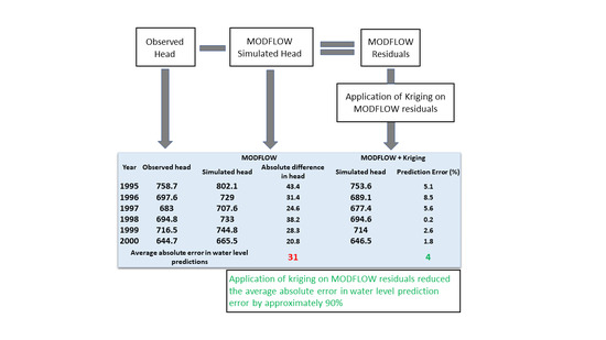
  • Mapping MODFLOW simulated groundwater heads (model imported from TWDB) into their corresponding coordinates and overlap with observation data to find the MODFLOW estimated values in the observation point.
  • Subtracting the observed groundwater head with MODFLOW simulated head and consider as the model residuals.
  • Dividing the residuals into two separate datasets, 90 percent of data for fitting kriging methods (calibrating residuals) and 10 percent for validating part (validating residuals), in a random selection.
  • Pre-evaluating the calibrating residuals and fit kriging method to generate the estimated residual map for the study domain.
  • Comparing the validating residuals with an estimated one to evaluate the accuracy of the kriging method.

2.3.1. Data Preparation

To minimize the distortion of the area and appropriate evaluation of the data, the NAD 1983 Texas Centric Mapping System Albers was used. First, the data were categorized into two groups—observed data and MODFLOW generated output. The observed data consists of the mean values for the water tables during the winter season (winter months were selected as the water tables are expected to be more stable during winter and thus minimize the anthropogenic effects due to uncertainties in demand seasons). The observed data were then provided with coordinates and transformed into a shapefile. For the MODFLOW generated data, the model grid shapefile produced by the MODFLOW program was employed in the study area and saved based on the needed attributes for future analysis. The binary files consisting of groundwater head data were converted to a text file using python programming. The extracted head data were matched with the corresponding observed data by locating the observation data in the grid shapefile. Finally, the shapefile of observation data was overlaid on the MODFLOW grid shapefile to determine the value of the MODFLOW generated head for each observation point. The MODFLOW generated heads were compared with the observed data for the corresponding locations thus obtaining the residuals.

2.3.2. Kriging Method

Kriging is one of the well known methods of predicting spatial characteristics and it has been used in a variety of fields (e.g., soil science, ecology, mining, and water resources) to provide a robust unbiased estimation of geo-distributed variables from small scales like X-ray scattering experiments [31] to large ones like traffic behavior pattern [32], soil properties’ profile [33], and anticipating the metrological variables [34]. The main advantage of the kriging method over the other spatial interpolation techniques is that the method is driven based on the statistical theory, comparing others that are mostly deterministic and they have the lack of ability to use for prediction. Furthermore, studies over geo-dependent variables showed that kriging has outstanding performance compared with its similar existing interpolation methods [35].
Equation (1) shows the stochastic function that is considered in the simple kriging method:
Z ( s ) = μ + ε ( s )
where Z ( s ) is the estimating function—which is simulated groundwater head elevation in our study, μ is a constant value representing the mean value of the groundwater head and ε ( s ) is a random error function regarding the model error from the observed records.
Estimating the value of Z ( s ) relies on two primary assumptions of considering that variables are randomly distributed, and they preserve second-order stationary condition respect to the location [36], which means:
E [ Z ( s + h ) ] = E [ Z ( s ) ]
c o v [ Z ( s + h ) ,   Z ( s ) ] = C [ h ]
where h is a vector that connects point s to point s + h. Equation (2) implies that the expected value E [ Z ( s ) ] is constant in all domains as represented in Equation (1) by the constant μ . However, in reality, this value fluctuates from place to place due to inherent trends and variability in data. To deal with this problem, it is usually assumed that the estimating variable (groundwater head) comprises two components
Z ( s ) = m ( s ) + e ( s )
where m ( s ) presents the deterministic part and e ( s ) is the statistical component of the estimating variable which includes the spatially correlated random variable. Since m ( s ) is treated as a deterministic part, it can be determined in a separate process and summed up with residuals random function component e ( s ) . In this study, the deterministic part of the head variable is estimated by existing numerical models. We then applied the ordinary kriging (OK) to the residuals of the numerical model for the statistical part assuming the mean value of error is not known and needs to be obtained over optimization process by minimizing the variance of errors.

3. Results and Discussion

3.1. Data Investigation

In standard statistical problems, the first step before starting to model the phenomena is to examine the data. In this study, a commonly used statistical tool, histogram, was used to see if the MODFLOW residuals are normally distributed. As shown in Figure 4, the residuals in general, follow the normality pattern. However, some level of negative skewness and distortion of normality was observed in the data which could be attributed to the complexity of nature.
Next, the residuals were checked for spatial correlation as the data tends to share some information with their neighbors. A variogram method was used to estimate how strongly data are related to each other. The variogram in space is usually implemented to check two major assumptions in the application of the kriging method—stationary in space (variance is independent of location) and isotropy (variance is independent of direction). Thus, a semi-variogram cloud or plot was used to provide a better visual understanding of the data distribution and to detect any possible trends or geometric anisotropic behavior.
Figure 5 shows the semi-variogram clouds of water level residuals calculated from subtraction between observation points and the MODFLOW outputs for the years 1995 to 2000. The difference squared ( γ ) in Figure 5 represents the MODFLOW residuals dissimilarity which is defined as:
γ = 1 2 ( Z ( s i ) Z ( s j ) ) 2
where s is sample location and Z is the residual value.
The reddish circles in the figure indicate that there is a strong gradient observed at short distances, as the value of the semi-variogram for each pair in these areas is significantly high. This significant change can be an indication of non-stationarity in higher ranks caused by neighboring drainage areas or rivers. However, to get a proper conclusion over the sources that resulted in non-stationary, more investigation needs to be considered which is beyond the scope of this study.
The semi-variogram was further used for interpolation where semi-variance was used to represent the expected value of the residuals’ dissimilarity. A theoretical model was fit into the sample data. In this study, a commonly used Spherical function was used. The spherical function shows a progressive decrease of spatial autocorrelation until some distance (radius of influence), beyond which autocorrelation is zero [37]. As observed from the sample variogram in Figure 6, the Nugget variance of 50 and range of 50,000 was defined for fitted theoretical semi-variogram.

3.2. Model Simulation

The ordinary Kriging method was applied to the MODFLOW residuals. In the process, the existing trend arising from uncertainties of the simulated model was removed using first-order trend and the exponential Kernel function was applied to weight the values of the neighbors closed to sampled values [38].
The spherical model was chosen to fit on a semi-variogram, and the maximum number of neighbors affecting the predicted data was limited to ten points. The kriging then applied as a single model resulted in a higher mean root square error (not presented in this paper), thus the area was divided into four quadrants with 45 offsets to minimize the distortion due to anisotropy as observed in Figure 5.
Figure 7 shows the prediction for OK applied to Edwards–Trinity aquifer between the years 1995 to 2000. High residuals (as shown by dark red and blue color) were observed for the areas outside the boundary while the residual values are minimal inside the study area. Furthermore, similar observations were observed in deviations as shown in Figure 8. The high residuals or larger deviation (as shown by purple color) outside the boundary is attributed to the missing observation data. Furthermore, some areas inside the study area showed relatively higher residuals with larger deviations which could also be due to the missing observation data.

3.3. Model Validation

As mentioned before, the entire dataset was divided into two sets—a simulation dataset (90% data) and a validation dataset (remaining 10% data). First, kriging was applied on 90% of the data where the validation was performed automatically using the ArcGIS Geostatistical Analyst toolbar [38]. The Geostatistical Analyst toolbar provides the measured and predicted values and the standard error for each point. During the process, the software keeps any individual points separate from other data (referred to as dataset) for estimating the spherical model parameters. The parameters are then estimated using every such dataset and the process continues until optimal parameters that best fit the entire datasets are obtained. Table 1 presents the average water head for observation points along with predicted water heads using MODFLOW and kriging, while Table 2 provides a detailed summary of kriging application on the MODFLOW residuals. As observed in Table 1, the residuals obtained from the MODFLOW simulation are much higher as compared to the residuals obtained after the application of kriging. The residuals significantly reduced from an average value of approximately 37 m to less than 1 m, with a standard error of approximately 0.5 m.
As a next step, a manual cross-validation was adopted where the calibrated model was applied to the remaining 10% of the data. Table 3 presents the average water heads for observation points along with predicted water heads using MODFLOW and kriging. Similar to observations in Table 1, higher residuals were obtained for the MODFLOW simulation for all the years. However, after the application of kriging on MODFLOW residuals, the average absolute error of approximately 31 m (from MODFLOW simulation) was reduced to less than 5 m. A similar reduction was observed in the residuals’ average standard error where the values reduced from 9.7 to 4.7. The observed reduction in standard error thus indicates that the average value of residuals over the entire period can be a good estimation for each year separately. Table 4 provides a detailed summary of the kriging application on the residuals.
For all the years, the water head for observation points obtained after kriging is much closer to the observed values. However, for the year 2000, three observation points (11, 12, and 15) showed higher residuals after the application of kriging as shown in Table 5. This could possibly be due to the higher prediction accuracy of the MODFLOW simulation in those points. The table with water heads for all the years (1995 through 2000) has been provided as a supplementary file in Table S1.

3.4. Comparison to Other Studies

The integrated approach used in this study satisfactorily described the general pattern of residuals generated by numerical model MODFLOW, thereby improving the prediction of the groundwater level at ungauged areas. Results showed that the integrated kriging and MODFLOW method can be used as an alternative approach in improving the existing numerical models whilst reducing the underlying model uncertainties. Most of the previous studies focused on decreasing the uncertainties by improving the resolution, or/and including local hydraulic variables like pumping and recharge/discharge to the large-scaled models [39].
However, the uncertainties in residuals can have sources of randomness that the improvements in the modeling process may not address, and rather could be represented by statistical methods such as kriging. The applied ordinary kriging in this study showed that the MODFLOW model’s residuals are locally correlated noises and can be estimated from their neighbors to some extent (with the range of 50 km) by using the spherical method as a correlation function. The numerical model used in this study was developed and improved by Anaya & Jones [29] and is the MODFLOW model approved by TWDB for the Edwards–Trinity Aquifer. In this study, MODFLOW was used as a deterministic part and the model uncertainties were presented as trends during the kriging model. The use of kriging reduced the average absolute error from approximately 31 m (from MODFLOW simulation) to less than 5 m after the application of kriging, which aligns with the findings from a previous study by Liu et al., [40]. They calibrated the MODFLOW model and were able to reduce the average absolute error from 7.7 m to 3.44 m through updates in the numerical modeling process. During the calibration process, they revised the recharge and used the actual value for pumping. However, the improvement was only performed for a smaller region (only the San Antonio segment of the aquifer) in contrast to improvement over the entire Edwards–Trinity as in the study presented by the authors.

4. Conclusions

The kriging method was applied to improve spatial confidence in groundwater-level predictions at unsampled locations. Kriging was applied on the MODFLOW residuals for the groundwater levels in the Edwards–Trinity aquifer in Texas. The study was done for the years 1995 through 2000 where 90% of the observation data was used for model simulation followed by validation with the remaining 10% of the observations. The kriging method significantly improved water level predictions. The average absolute error of approximately 31 m (from MODFLOW simulation) was reduced to less than 5 m after the application of kriging on MODFLOW residuals. Furthermore, the average residuals’ standard error decreased from 9.7 to 4.7, which indicates that the average value of residuals over the entire period can be a good estimation for each year separately. With improved water level predictions, geostatistical tools such as kriging can be used to produce more accurate potentiometric surface maps. Such improved results and accurate monitoring of groundwater resources will lead to the sustainable use of groundwater resources while also aiding in efficient and effective conjunctive management of surface and groundwater resources.

Supplementary Materials

The following are available online at https://www.mdpi.com/article/10.3390/w14030426/s1, Table S1: Predicted water head for observation points for the the years 1995 through 2000.

Author Contributions

Conceptualization, A.A. and K.A.; methodology, A.A.; validation, K.A.; formal analysis, A.A. and K.A.; investigation, A.A. and K.A.; data curation, A.A.; writing—original draft preparation, A.A. and K.A.; writing—review and editing, A.A. and K.A.; visualization, A.A. and K.A.; funding acquisition, K.A. All authors have read and agreed to the published version of the manuscript.

Funding

The manuscript hasn‘t receive external founding. Publishing fee for this article has been covered by College of Natural Sciences at Cal Poly Humboldt.

Data Availability Statement

Data available on request.

Acknowledgments

The authors would like to thank the Department of Civil, Environmental and Construction Engineering at Texas Tech University for their support in conducting this research with assistantship support. And, sincere thanks to Guofeng Cao fromthe Department of Geography at University of Colorado, Boulder, and Adjunct Faculty of the Department of Geography at Texas Tech University, for his guidance with the research.

Conflicts of Interest

The authors declare no conflict of interest.

References

  1. Adhikari, K.; Fedler, C.B. Water sustainability using pond-in-pond wastewater treatment system: Case studies. J. Water Process Eng. 2020, 36, 101281. [Google Scholar] [CrossRef]
  2. Adhikari, K.; Fedler, C.B. Pond-In-Pond: An alternative system for wastewater treatment for reuse. J. Environ. Chem. Eng. 2020, 8, 103523. [Google Scholar] [CrossRef]
  3. Mehan, G.T., III; Scientific American. The EPA Says We Need to Reuse Wastewater. 2019. Available online: https://blogs.scientificamerican.com/observations/the-epa-says-we-need-to-reuse-wastewater/ (accessed on 11 December 2019).
  4. FAO. AQUASTAT Main Database, Food and Agriculture Organization of the United Nations (FAO). 2018. Available online: http://www.fao.org/nr/water/aquastat/didyouknow/index.stm (accessed on 26 January 2022).
  5. FAO. AQUASTAT Main Database, Food and Agriculture Organization of the United Nations (FAO). 2016. Available online: http://www.fao.org/nr/water/aquastat/data/query/index.html?lang=en (accessed on 26 January 2022).
  6. NGWA. The Groundwater Association. 2020. Available online: https://www.ngwa.org/what-is-groundwater/About-groundwater/information-on-earths-water (accessed on 26 January 2022).
  7. Fendekova, M.; Demeterova, B.; Slivova, V.; Macura, V.; Fendek, M.; Machlica, A.; Gregor, M.; Jalcovikova, M. Surface and groundwater drought evaluation with respect to aquatic habitat quality applied in Torysa river catchment, Slovakia. Ecohydrol. Hydrobiol. 2011, 11, 49–61. [Google Scholar] [CrossRef]
  8. Lange, B.; Holman, I.; Bloomfield, J.P. A framework for a joint hydro-meteorological-social analysis of drought. Sci. Total Environ. 2017, 578, 297–306. [Google Scholar] [CrossRef] [Green Version]
  9. Chakraborty, S.; Maity, P.K.; Das, S. Investigation, simulation, identification and prediction of groundwater levels in coastal areas of Purba Midnapur, India, using MODFLOW. Environ. Dev. Sustain. 2020, 22, 3805–3837. [Google Scholar] [CrossRef]
  10. Hutchison, W.R.; Jones, I.; Anaya, R. Update of the Groundwater Availability Model for the Edwards-Trinity (Plateau) and Pecos Valley Aquifers of Texas; Unpublished Report; Texas Water Development Board: Austin, TX, USA, 2011. [Google Scholar]
  11. Xue, S.; Yu Liu, S.L.; Li, W.; Wu, Y.; Pei, Y. Numerical simulation for groundwater distribution after mining in Zhuanlongwan mining area based on visual MODFLOW. Environ. Earth Sci. 2018, 77, 400. [Google Scholar] [CrossRef]
  12. Tapoglou, E.; Karatzas, G.P.; Trichakis, I.C.; Varouchakis, E.A. A spatio-temporal hybrid neural network-Kriging model for groundwater level simulation. J. Hydrol. 2014, 519, 3193–3203. [Google Scholar] [CrossRef]
  13. Theodossiou, N.; Latinopoulos, P. Evaluation and optimisation of groundwater observation networks using the Kriging methodology. Environ. Model. Softw. 2006, 21, 991–1000. [Google Scholar] [CrossRef]
  14. Marchant, B.P.; Bloomfield, J.P. Spatio-temporal modelling of the status of groundwater droughts. J. Hydrol. 2018, 564, 397–413. [Google Scholar] [CrossRef]
  15. Oikonomou, P.D.; Alzraiee, A.H.; Karavitis, C.A.; Waskom, R.M. A novel framework for filling data gaps in groundwater level observations. Adv. Water Resour. 2018, 119, 111–124. [Google Scholar] [CrossRef]
  16. Varouchakis, Ε.; Hristopulos, D. Comparison of stochastic and deterministic methods for mapping groundwater level spatial variability in sparsely monitored basins. Environ. Monit. Assess. 2013, 185, 1–19. [Google Scholar] [CrossRef] [PubMed]
  17. Ruybal, C.J.; Hogue, T.S.; McCray, J.E. Evaluation of groundwater levels in the Arapahoe aquifer using spatiotemporal regression kriging. Water Resour. Res. 2019, 55, 2820–2837. [Google Scholar] [CrossRef]
  18. Ziolkowska, J.R.; Reyes, R. Groundwater level changes due to extreme weather—An evaluation tool for sustainable water management. Water 2017, 9, 117. [Google Scholar] [CrossRef] [Green Version]
  19. Kuria, D.N.; Gachari, M.K.; Macharia, M.W.; Mungai, E. Mapping groundwater potential in Kitui District, Kenya using geospatial technologies. Int. J. Water Resour. Environ. Eng. 2011, 4, 15–22. [Google Scholar]
  20. Minor, T.B.; Russell, C.E.; Mizell, S.A. Development of a GIS-based model for extrapolating mesoscale groundwater recharge estimates using integrated geospatial data sets. Hydrogeol. J. 2007, 15, 183–195. [Google Scholar] [CrossRef]
  21. Aboufirassi, M.; Mariño, M.A. Kriging of water levels in the Souss aquifer, Morocco. J. Int. Assoc. Math. Geol. 1983, 15, 537–551. [Google Scholar] [CrossRef]
  22. Pucci, A.A., Jr.; Murashige, J.A.E. Applications of universal kriging to an aquifer study in New Jersey. Groundwater 1987, 25, 672–678. [Google Scholar] [CrossRef]
  23. Hoeksema, R.J.; Clapp, R.B.; Thomas, A.L.; Hunley, A.E.; Farrow, N.D.; Dearstone, K.C. Cokriging model for estimation of water table elevation. Water Resour. Res. 1989, 25, 429–438. [Google Scholar] [CrossRef]
  24. Desbarats, A.J.; Logan, C.E.; Hinton, M.J.; Sharpe, D.R. On the kriging of water table elevations using collateral information from a digital elevation model. J. Hydrol. 2002, 255, 25–38. [Google Scholar] [CrossRef]
  25. Olea, R.; Davis, J. Optimaizing the High Plains Aquifer Water-Level Observation Network; Kansas Geological Surveying: Lawrence, KS, USA, 1999. [Google Scholar]
  26. Ahmadi, S.H.; Sedghamiz, A. Geostatistical analysis of spatial and temporal variations of groundwater level. Environ. Monit. Assess. 2007, 129, 277–294. [Google Scholar] [CrossRef]
  27. Ahmadi, S.H.; Sedghamiz, A. Application and evaluation of kriging and cokriging methods on groundwater depth mapping. Environ. Monit. Assess. 2008, 138, 357–368. [Google Scholar] [CrossRef] [PubMed]
  28. Rivest, M.; Marcotte, D.; Pasquier, P. Hydraulic head field estimation using kriging with an external drift: A way to consider conceptual model information. J. Hydrol. 2008, 361, 349–361. [Google Scholar] [CrossRef]
  29. Anaya, R.; Jones, I. Groundwater Availability Model for the Edwards-Trinity (Plateau) and Pecos Valley Aquifers of Texas; Texas Water Development Board: Austin, TX, USA, 2009. [Google Scholar]
  30. Texas Water Development Board, Groundwater Models. Available online: https://www.twdb.texas.gov/groundwater/models/alt/eddt_p_2011/alt1_eddt_p.asp (accessed on 11 May 2020).
  31. Noack, M.M.; Yager, K.G.; Fukuto, M.; Doerk, G.S.; Li, R.; Sethian, J.A. A kriging-based approach to autonomous experimentation with applications to X-ray scattering. Sci. Rep. 2019, 9, 11809. [Google Scholar] [CrossRef] [PubMed] [Green Version]
  32. Pinto, J.A.; Kumar, P.; Alonso, M.F.; Andreao, W.L.; Pedruzzi, R.; Espinosa, S.I.; Albuquerque, T.T. Kriging method application and traffic behavior profiles from local radar network database: A proposal to support traffic solutions and air pollution control strategies. Sustain. Cities Soc. 2020, 56, 102062. [Google Scholar] [CrossRef]
  33. Gotway, C.A.; Ferguson, R.B.; Hergert, G.W.; Peterson, T.A. Comparison of kriging and inverse-distance methods for mapping soil parameters. Soil Sci. Soc. Am. J. 1996, 60, 1237–1247. [Google Scholar] [CrossRef]
  34. Venäläinen, A.; Heikinheimo, M. Meteorological data for agricultural applications. Phys. Chem. Earth Parts A/B/C 2002, 27, 1045–1050. [Google Scholar] [CrossRef]
  35. Laslett, G.M. Kriging and splines: An empirical comparison of their predictive performance in some applications. J. Am. Stat. Assoc. 1994, 89, 391–400. [Google Scholar] [CrossRef]
  36. Wackernagel, H. Multivariate Geostatistics: An Introduction with Applications; Springer Science & Business Media: Berlin, Germany, 2013. [Google Scholar]
  37. esri. How Kriging Works. 2021. Available online: https://pro.arcgis.com/en/pro-app/latest/tool-reference/3d-analyst/how-kriging-works.htm (accessed on 26 January 2022).
  38. ArcGIS Desktop. 2021. Available online: https://desktop.arcgis.com/en/arcmap/latest/extensions/geostatistical-analyst/what-is-arcgis-geostatistical-analyst-.htm (accessed on 26 January 2022).
  39. Sharp, M.J., Jr.; Green, R.T.; Schindel, G.M. The Edwards Aquifer: The Past, Present, and Future of a Vital Water Resource; Geological Society of America: Boulder, CO, USA, 2019; Volume 215. [Google Scholar]
  40. Liu, A.; Troshanov, N.; Winterle, J.; Zhang, A.; Eason, S. Updates to the MODFLOW Groundwater Model of the San Antonio Segment of the Edwards Aquifer; Edwards Aquifer Authority: San Antonio, TX, USA, 2017. [Google Scholar]
Figure 1. Location of the study area—Edwards–Trinity (Plateau) Aquifer.
Water 14 00426 g001
Figure 2. Location of observation wells in the Edwards–Trinity aquifer.
Water 14 00426 g002
Figure 3. Schematic diagram of the MODFLOW + kriging model.
Water 14 00426 g003
Figure 4. Histogram presenting the water level residuals for Edwards–Trinity aquifer (years 1995–2000).
Water 14 00426 g004
Figure 5. Semi-variogram cloud for water level residuals during the years 1995 through 2000.
Water 14 00426 g005
Figure 6. Sample variogram and fitted model applied on Edwards aquifer dataset for years 1995 through 2000.
Water 14 00426 g006
Figure 7. Predicted residuals (in meters) after application of kriging on MODFLOW residuals for years 1995 through 2000.
Water 14 00426 g007
Figure 8. Standard Deviation (in meters) for ordinary kriging applied to Edwards–Trinity aquifer for the years 1995 through 2000 (the black dots in the figure represent the observation points used during cross-validation).
Water 14 00426 g008
Table 1. Average water heads using MODFLOW and kriging method (simulation dataset).
YearObservations 1MODFLOW (m)MODFLOW + Kriging (m)
Mean a 2Observed Residuals 3Standard Error Mean b 4Predicted Residuals 5Error 6Standard Error
1995727.5764.7−37.23.1728.7−361.20.7
1996665.5706−40.53.3667.1−38.91.60.4
1997692.4725.5−33.12.9693.5−321.10.4
1998682.4716.6−34.22.9682.8−33.80.40.5
1999708.3747.1−38.82.9708.6−38.50.30.3
2000686724.7−38.73.2685.3−39.4−0.71.1
1 Observed average value for water level for the given year (winter season). 2 MODFLOW simulated average value for water level for the given year (winter season). 3 Difference between observed values and the MODFLOW simulated values (Observations—Mean a). 4 Simulated average value for water level for the given year after application of kriging (Mean a + Predicted Residuals). 5 Residuals obtained after application of kriging on the observed residuals. 6 Difference between predicted and observed residuals for each point.
Table 2. Detailed summary of kriging application on MODFLOW residuals (simulation dataset).
Year Min.1st Qu.MedianMean3rd Qu.Max.
1995Observed Residuals−141.6−53.1−32.2−37.2−20.855.2
Predicted Residuals−147.1−52.1−31.9−36−22.552.3
Error−97.3−6.7−0.11.25.284.5
Standard Error0.40.70.80.70.80.8
1996Observed Residuals−137.1−60.8−40.9−40.5−16.130.4
Predicted Residuals−132.7−56.8−43.3−38.9−14.333.6
Error−49.6−6.40.81.611.672.8
Standard Error0.40.40.40.40.40.4
1997Observed Residuals−135.4−51.7−32.6−33.1−11.362.5
Predicted Residuals−148.1−47−31.7−32−9.145.7
Error−59−6.40.517.778
Standard Error0.20.40.40.40.40.5
1998Observed Residuals−131−54.3−32.3−34.2−16.964
Predicted Residuals−145.8−53.2−33.4−33.8−19.343.8
Error−50−8.70.40.47.161.3
Standard Error0.40.50.50.50.50.5
1999Observed Residuals−144.6−54−31.7−38.8−18.452.5
Predicted Residuals−150−53.1−31.1−38.5−20.952.2
Error−55.2−8.20.40.37.775.9
Standard Error0.30.30.30.30.30.3
2000Observed Residuals−141.1−59.3−35.7−38.7−15.848
Predicted Residuals−139.3−56.4−39.5−39.4−19.136.1
Error−79.7−8.70−0.78.366.2
Standard Error0.41.21.21.11.21.3
Table 3. Average water heads using MODFLOW and kriging method (validation dataset).
YearObservationsMODFLOW (m)MODFLOW + Kriging (m)
MeanObserved ResidualsStandard ErrorMeanPredicted ResidualsErrorStandard Error
1995758.7802.1−43.58.7753.6−48.5−5.13
1996697.6729−31.414.7689.1−39.9−8.55.3
1997683707.6−24.65.9677.4−30.1−5.53.9
1998694.8733−38.110.7694.6−38.3−0.28.1
1999716.5744.8−28.38.4714−30.8−2.53.8
2000644.7665.5−20.810646.5−191.84.6
Table 4. Detailed summary of kriging application on MODFLOW residuals (validation dataset).
Year Min.1st Qu.MedianMean3rd Qu.Max.
1995Observed Residuals−131.8−50−33.9−43.5−24−15
Predicted Residuals−132.5−55−31.8−48.5−24.8−18.9
Error−7.1−1.30.85.18.929.3
Standard Error---3--
1996Observed Residuals−138.1−55.2−30.1−31.4−1.861
Predicted Residuals−143.1−46.5−37.2−40−5.340.3
Error−20.5−5.258.520.352.1
Standard Error---5.3--
1997Observed Residuals−82.3−36.6−28.1−24.6−6.916.2
Predicted Residuals−80.9−44.9−31.1−30.2−7.316.7
Error−18.5−3.105.520.638.7
Standard Error---3.9--
1998Observed Residuals−134.5−56.6−33.7−38.1−25.262
Predicted Residuals−76.3−51.7−45−38.3−22.5−10.1
Error−87.3−60.80.210.472.9
Standard Error---8.1--
1999Observed Residuals−68.1−54.8−33.6−28.3−19.365.5
Predicted Residuals−71−52.1−39.1−30.8−22.832
Error−38.6−2.70.32.59.735.8
Standard Error---3.8--
2000Observed Residuals−120.5−46.4−16.2−20.8−3.265.6
Predicted Residuals−71.7−45.9−20.4−19.14.241
Error−48.9−40.5−1.710.224.7
Standard Error---4.6--
Table 5. Predicted water heads for observation points for the year 2000.
Observation WellObserved Head (m)MODFLOW (m)MODFLOW + Kriging (m)
Simulated HeadResidualsPredicted HeadResiduals
1769786.9−17.9764.44.6
2745.7760.1−14.4741.83.8
3748.3868.8−120.5797.2−48.9
41059.2993.665.61034.624.7
5662.2713.2−50.9652.310
6548.9595.9−47552.5−3.6
7586.6608.2−21.6574.712
8648.8695−46.2647.21.6
9585617.7−32.6570.114.9
10616.1663.8−47.7618.4−2.3
11613.4619.5−6.2602.211.1
12618.5623.3−4.8629.4−10.9
13623.6620.63624.1−0.5
14588.9568.320.5594−5.1
15555.1568.4−13.3593−37.8
16346.3344.71.6347.4−1.2
Publisher’s Note: MDPI stays neutral with regard to jurisdictional claims in published maps and institutional affiliations.

