Using Time-Lapse Resistivity Imaging Methods to Quantitatively Evaluate the Potential of Groundwater Reservoirs

Abstract

In this study, we attempt to establish an alternative method for estimating the groundwater levels and the specific yields of an unconfined aquifer for the evaluation of potential groundwater reservoirs. We first converted the inverted resistivity into the normalized water content. Then, we inverted the parameters of the Brooks-Corey model from the vertical profiles of the water content by assuming that the suction head was in proportion to the elevation regarding a predefined base level. Lastly, we estimated the groundwater level, the theoretical specific yield, and the specific yield capacity from the Brooks-Corey parameters at every survey site in the study area. The contour maps of the time-lapse groundwater levels show that the groundwater flows downstream, with a higher hydraulic gradient near the river channel than in the area away from the main channel. We conclude that the estimated maximum specific yield capacities are consistent with that derived from the pumping tests in the nearby observation well. Additionally, the specific yield capacities are only three quarters to two thirds of the theoretical specific yields derived from the difference between the residual and saturated water contents in the Brooks-Corey model. We conclude that the distribution pattern of the specific yields had been subjected to the distribution of natural river sediments in the Minzu Basin, since the modern channel was artificially modified. Although we had to make some simple assumptions for the estimations, the results show that the surface resistivity surveys provide reasonable estimations of the hydraulic parameters for a preliminary assessment in an area with few available wells.

1. Introduction

Climate change has boosted the frequency of extreme weather events, such as floods and droughts. To cope with the water shortage from super-drought events, it is feasible to store excess surface water during the wet season in subsurface reservoirs, i.e., groundwater reservoirs, for use in the drought seasons. As a result, it is important to know the suitable areas for potential groundwater reservoirs. To quickly evaluate the potential of groundwater reservoirs, we developed an alternative method for applying time-lapse resistivity measurements to groundwater-level estimations. We estimated the specific yields of an unconfined aquifer in the Minzu Basin in central Taiwan. The basin consists of thick gravel layers and is considered to be a potential groundwater reservoir. However, there are few borehole records for the basin and, therefore, we were able to use only non-destructive geophysical methods for our evaluation. Several studies have used qualitative resistivity methods to identify groundwater-related physical and chemical properties. For example, Michot and Benderitter [1] used resistivity surveys to monitor the variations in soil-based water content. Berthold and Bentley [2] integrated hydrogeology and geophysics in the Canadian plains for groundwater replenishment research. Additionally, Rayner and Bentley [3] used resistivity imaging methods to determine the hydrogeological settings of aquifers in fractured rocks. Recently, researchers have turned their attention to quantitative estimations of hydrogeological parameters. These estimations rest on low-cost, non-destructive geophysical methods, especially the surface resistivity method. Frohlich and Kelly [4] used Archie’s law and one-dimensional resistivity results to derive specific yields based on resistivity measurement differences in saturated and unsaturated layers. To calculate specific yields, Dietrich and Carrera [5] used a similar approach with time-lapse two-dimensional resistivity surveys. With a simplified Archie’s law, they first transferred their inverted resistivity results into the water contents in soils, before calculating the differences in water volumes; then, the researchers estimated the specific yield by dividing the water volume change into the water-level difference, which itself had been calculated from the piezometer next to the survey line. Moreover, Chang and Chang [6] used time-lapse resistivity imaging during a pumping test to estimate the hydraulic conductivities and the specific yields of unconfined aquifers. The aforementioned results show that measured vertical resistivity changes can indicate the depths of groundwater tables, because they are consistent with drastic changes in resistivity.

The surface resistivity method provides an alternative way to appraise regional hydrogeological parameters when few or even zero observation wells are available for a direct calculation of these parameters. In the present study, we evaluate hydraulic parameters by further incorporating in situ surface resistivity measurements into soil-water characteristic models. Our aim is to acquire relative parameters that can be used for appraising potential groundwater reservoirs regarding, for example, regional groundwater depths and specific yields. Our attempted approach may constitute an alternative and effective method by which researchers can calculate regional hydrogeological parameters with limited available boreholes.

2. Materials and Methods

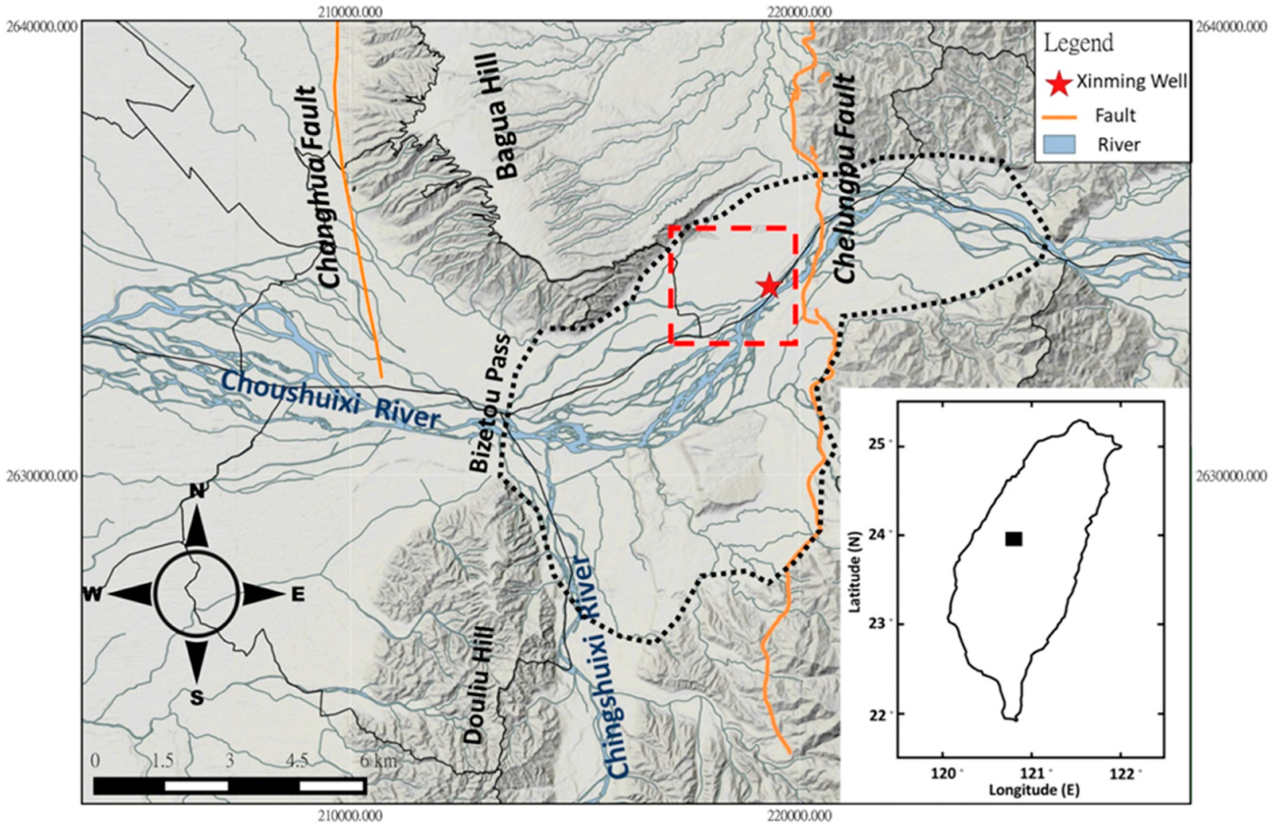
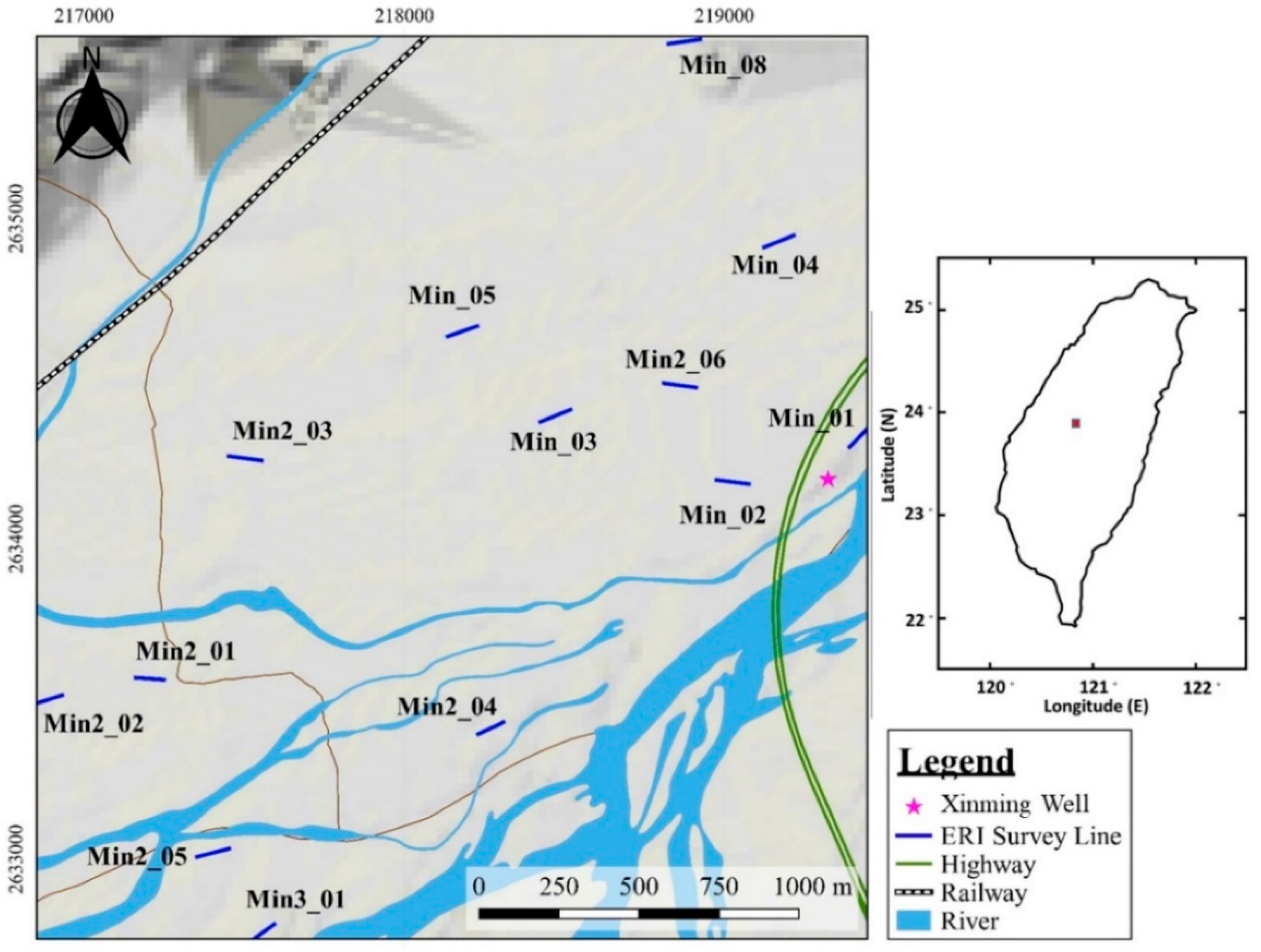
2.1. The Survey Area and the Design of the Electrical Resistivity Imaging

The annual precipitation in Taiwan is about 2500 mm/year, which is 2.5 times the global average rainfall. The weather records show a significant difference between the precipitation of the wet season (May to October) and dry season (November to April). Precipitation in the wet season accounts for 77% of annual precipitation in the central region of Taiwan, and typhoon events are the major sources of precipitation in the wet season [7]. However, it is projected that the precipitation amount in the wet season will be increased to over 82–88% of annual rainfall in the region by the end of the 21st century [8]. Hence, we have to look for an enhanced water management plan to meet the needs of dry seasons in the future.

Our survey area is located in the Minzu Basin in Nantou County in Central Taiwan (Figure 1).

The Minzu Basin is a piggyback basin formed by the foreland thrust faults, the Chelungpu Fault in the east and the Changhua Fault in the west. The Choushui River cuts through the parallel thrust faults and provides the area with sediment. The west side of the basin is connected to the Choushui River alluvial fan through the Bizetou Pass between the Bagua and Douliu hills, which were created by the Changhua thrust fault, whereas the east side is bounded by the Chelungpu thrust fault. The Chingshui River from the south merges into the Choushui River near the Bizetou Pass. Sediment from these rivers is deposited into the Minzu Basin. Because the bounding Changhua and Chelungpu faults are both westward thrusts, one would expect that the thickness of unconsolidated sediment in the basin may range from several meters in the east to over a hundred meters in the west. The sediment deposits are mainly composed of gravel and sand, and the subsequent loose structure has good permeability. Therefore, the Minzu Basin is regarded as an area with extremely high potential for groundwater recharge.

Our resistivity survey lines are set in the north bank of the Choushui River, and are roughly centered around the Xinming observation well, completed by the Central Geological Survey (CGS) of Taiwan. To obtain estimation results from the resistivity surveys, we used the Xinming well for calibration purposes. From the borehole records, the deposits that are 100 m deep mainly consist of sand and gravel with a logging resistivity higher than 100 Ohm-m in both the 16”and 64” measurements (Figure 2). Figure 3 presents the distribution of the survey lines. The orientations of survey lines are mostly parallel to the Choushui River, thus reducing the effects caused by the lateral variation from the river sedimentation. Owing to site-specific conditions, there are a few exceptions wherein the survey lines are not oriented in a parallel direction.

We conducted time-lapse surveys roughly every three months across the dry and wet seasons at the same survey sites using Wenner–Schlumberger configuration with a 1 m electrode interval. The data set includes data collected in December of 2016 (the dry season), in March of 2017 (the dry season), in June of 2017 (the wet season), in August of 2017 (the wet season), from the end of September to early October of 2017 (the wet season), in January of 2018 (the dry season), and in March of 2018 (the dry season). In December of 2016, we initiated pilot surveys at the Min_01, Min_02, Min_03, Min_04, Min_05, Min_06, and Min_08 sites. The pilot surveys were designed to help with the selection of proper sites; subsequently, we decided to discard the Min_07 site owing to its poor condition. Sites Min2_01, Min2_02, Min2_03, Min2_04, and Min2_06 were added as additional survey sites in March of 2017, and a further site, Min3_01 was added in June of 2017. The resistivity surveys were conducted at the aforementioned sites in August and September of 2017. The survey project was completed at the end of 2017, yet we decided to keep conducting resistivity surveys at the Min_01, Min_02, Min_03, Min_05, Min_06, Min2_01, Min2_02, and Min3_01 sites in January and March of 2018.

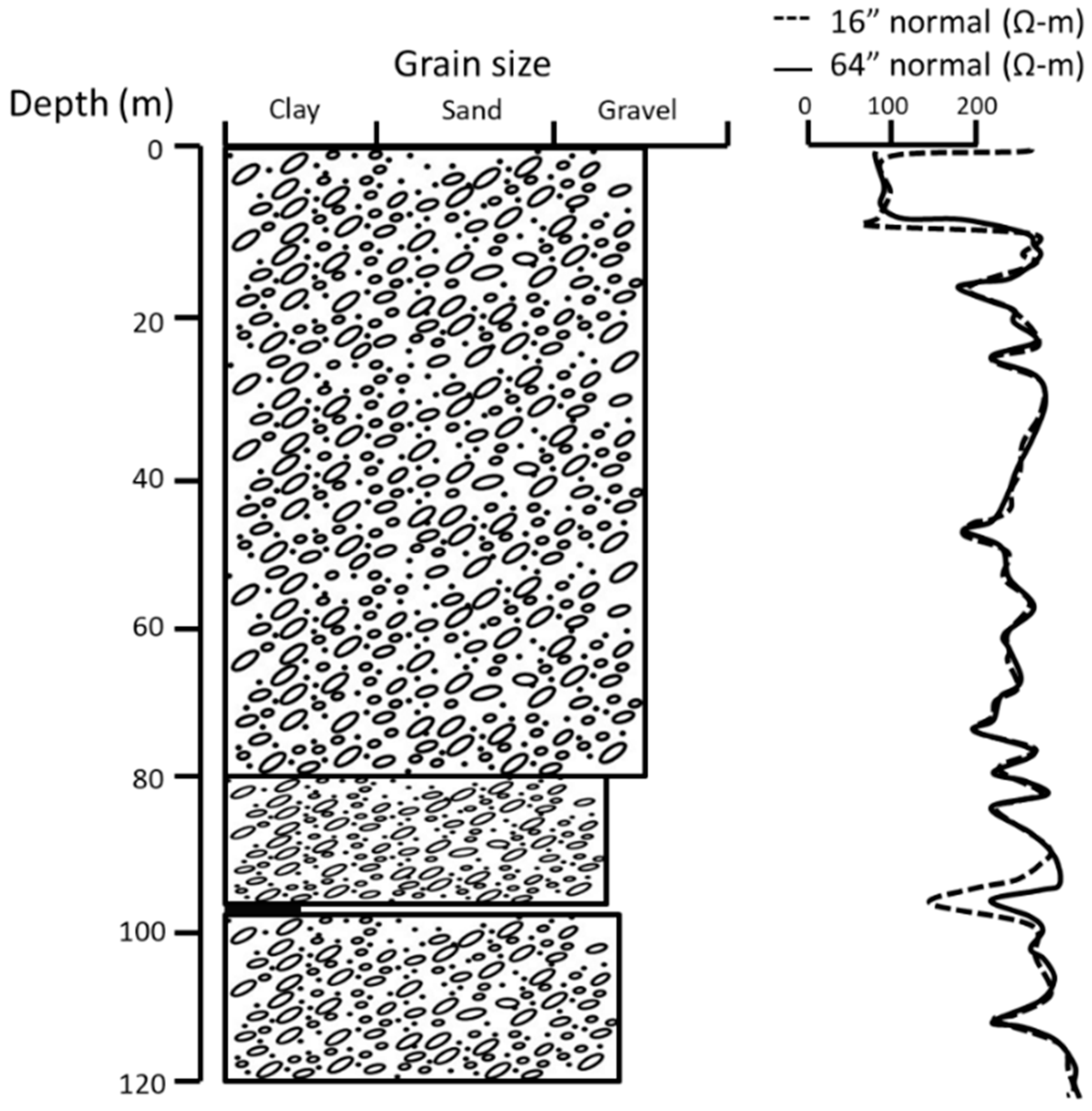
2.2. The Resistivity Survey and Depth Estimation for the Groundwater Table

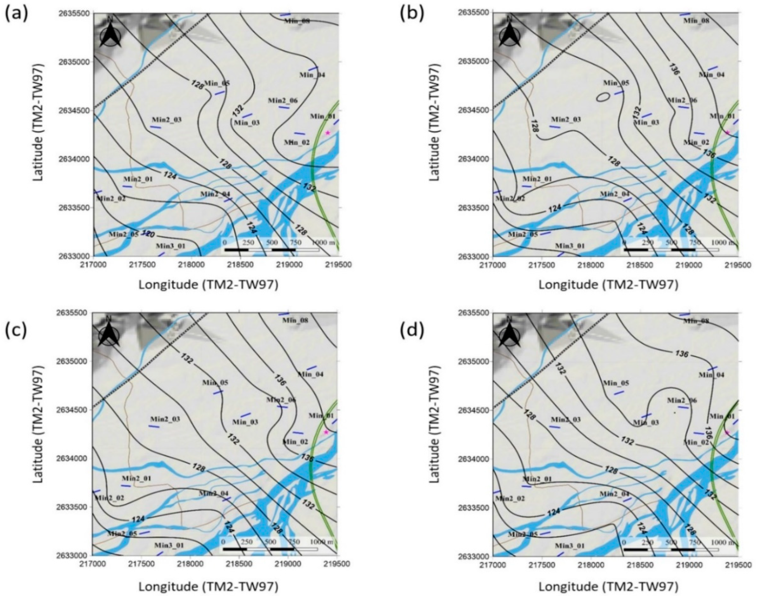
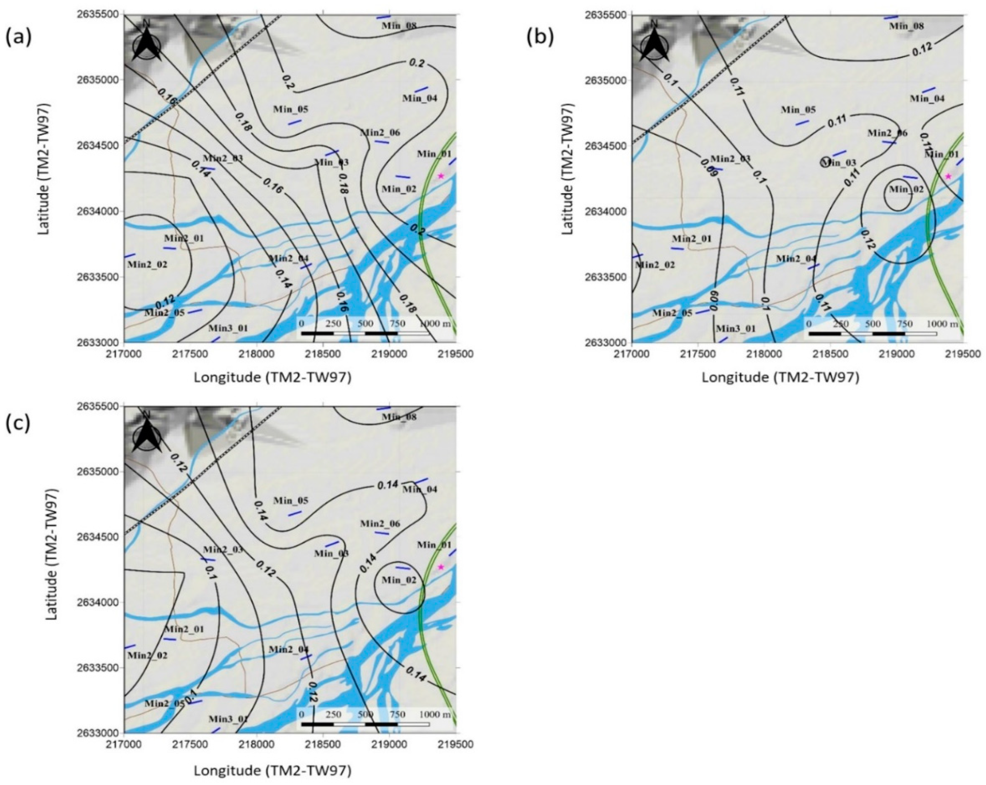
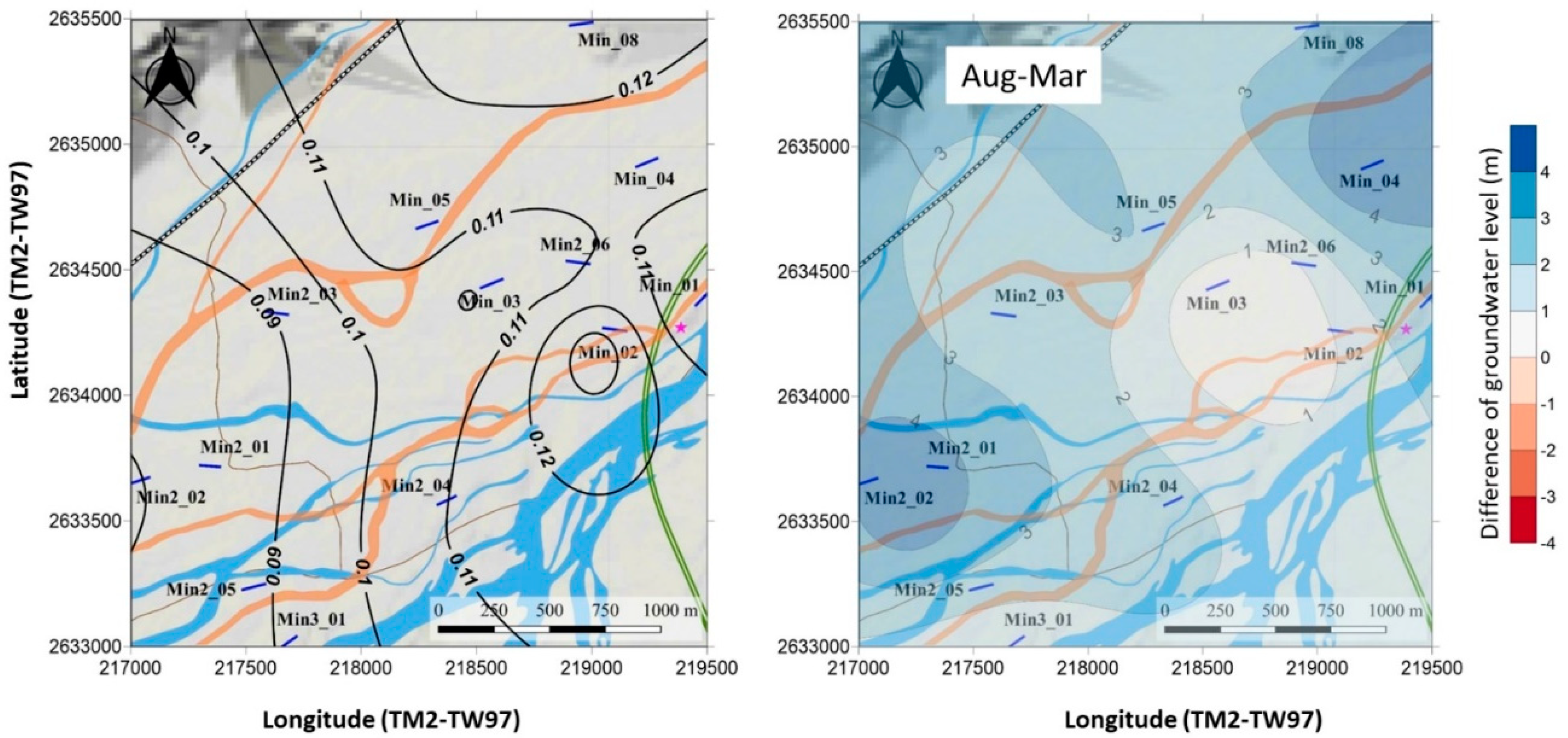
Resistivity exploration uses direct current or low-frequency alternating current to establish an artificial underground electric field with a pair of electrodes. One can measure the resulting field with another pair of electrodes to calculate the apparent resistivity. The measured apparent resistivity is the comprehensive effect of all the electrical strata under the corresponding electrode configurations. Therefore, a further inversion approach is needed to derive a subsurface resistivity model.

There are several physical factors that may affect the measured subsurface resistivity, including lithology, mineral composition, water content, porosity, pore structure and connectivity, pore water composition [9], and temperature variations [10]. One can measure subsurface resistivity for various ranges and depths by changing the aforementioned electrode configurations, including electrode distance, and the position and sequence of measurements. Each configuration, or array, has its own advantages and limitations in subsurface object detections. We forward readers to Zhou [11] for the comprehensive principles of the resistivity methods and array configurations.

We used the 4-point light 10 W resistivity meter and the active electrode (ActEle) system (Lippmann Geophysical Instruments (LGM), Schaufling, Bayern) [12] for the field data measurements. We chose the Wenner–Schlumberger arrays with 1 m electrode spacing for the present study data measurements, since they often yield high signal-to-noise ratios and have better sensitivity to horizontal structures [13,14]. The two-dimensional (2D) inverse software used in this research is the EarthImager2D^TM Version 2.4.2.627 (Advanced Geosciences Inc. (AGI), Austin, TX, USA) [15]. The EarthImager2D^TM involves finite-element forward solutions and an iterative conjugate gradient inversion scheme, both of which facilitate calculations of the optimal resistivity models [16,17]. A detailed review of the inversion techniques for resistivity surveys can be found in Sharma and Verma [18].

We adopted a similar procedure to Dietrich and Carrera [5] for estimating the water contents in a column profile at each survey sites. According to Archie’s Law [9], we can clarify how formation resistivity relates to porosity, saturation, and pore water resistivity for a clay-free matrix:

$${\rho }_t=\alpha {\rho }_w{\varphi }^{-n}{S}_w{}^{-m},$$

(1)

where ${\rho }_t$ is the formation resistivity, ${\rho }_w$ is the pore water resistivity, $\varphi$ is the porosity, $S_w$ is the saturation, and m and n are the saturation index and cementation index, respectively. Since the deposits mainly consist of sand and gravel within 100 m deep in our study area, according to the borehole records, we are able to use Equation (1) for the estimation of the hydrological parameters without applying the correction for clay surface conduction effects. For general homogeneous rocks and soils, m ranges from 1.8 to 2.2, and the value of n is about 2; thus, considering m = n ≅ 2, Equation (1) is approximated as:

$${\rho }_t=\alpha {\rho }_w{\theta }^{-2},$$

(2)

where $\theta$ is the volumetric water content.

Furthermore, if we assume that the sediment textures are homogeneous within the exploration ranges, and that resistivity varies only with the water saturation, we can obtain the normalized relative saturation, $S_r$, at different depths in the vadose zone:

$$S_r=\frac{{\theta }_u}{{\theta }_s}=\sqrt{\frac{{\rho }_s}{{\rho }_u}}.$$

(3)

In Equation (3), ${\theta }_u$ is the unsaturated water content, ${\rho }_u$ is the unsaturated layer formation resistivity, ${\theta }_s$ is the saturated layer volume water content, and ${\rho }_s$ represents the saturated layer formation resistivity.

If we can estimate the average porosity, i.e., ${\varphi }_A$, of soils or rocks from other experiments or particle size analysis data, we can further obtain the normalized volumetric water content:

$$\theta =S_r{\varphi }_A.$$

(4)

Figure 4 presents an example in which normalized volumetric water content varies from the ground surface to the saturated layer, as estimated from selected resistivity measurements in an unconfined aquifer.

The data of the topmost 2 m are excluded because they represent the properties of the surface soil layer instead of the properties of the gravel aquifer. The vertical change in the water content in Figure 4 exhibits a similar trend relative to the soil-water characteristic curve developed in lab experiments, e.g., [19,20]. Therefore, if we assume the suction head is linearly proportional to the elevation of the groundwater level in the unconfined aquifer, as discussed in Krahn and Fredlund [21], we would be able to accomplish two tasks: first, estimate the relative hydraulic parameters in the vadose zone [20], and second, estimate the groundwater level quantitatively with the soil-water characteristic model.

There are several empirical models, including the Brooks-Corey model [22] and the Van Genuchten model [23], that describe the physical relationships between the water contents and suction in the vadose zone. If we assume that the suction head in the unsaturated zone is proportional to the height of the groundwater level, we should use the Brooks-Corey model for the soil-water characteristic curves [22]:

$$\theta \left(h\right)=\{\begin{array}{c}\begin{array}{c} \\ {\theta }_r+\left({\theta }_s-{\theta }_r\right){\left(\frac{h_a}{h}\right)}^{\lambda }, for \frac{h_a}{h}<1\end{array}\\ {\theta }_s, for \frac{h_a}{h}\ge 1\end{array}$$

(5)

where θ(h) is the unsaturated water content (L³L⁻³), h is the suction head (L) and is approximated as the air entry height of the presumed groundwater table, ${\theta }_s$ is the saturated water content (L³L⁻³) and is set to be ${\varphi }_A$ in this case, ${\theta }_r$ is the residual water content (L³L⁻³), $\lambda$ is the Brooks-Corey parameter, and $h_a$ corresponds to the air entry suction head.

If we designate a saturated base with a depth of $H_s$ and assume that the suction head is proportional to the height of the presumed saturated base, we may estimate the apparent air entry suction head relative to the same base, $h_a$, with the Brooks-Corey model of soil-water characteristic curves. Hence, we can calculate the depth of the near-saturated surface of air entry suction, D, as:

$$D=H_s-h_a.$$

(6)

In reality, the true groundwater table may be lower than the surface corresponding to the air entry suction. Hence, we may apply the correction for the approximation if we can obtain the true groundwater depth from the observation well. We can then use the correction to construct the distribution of regional groundwater levels at places without wells. We will discuss the correction later in the discussion.

3. Results

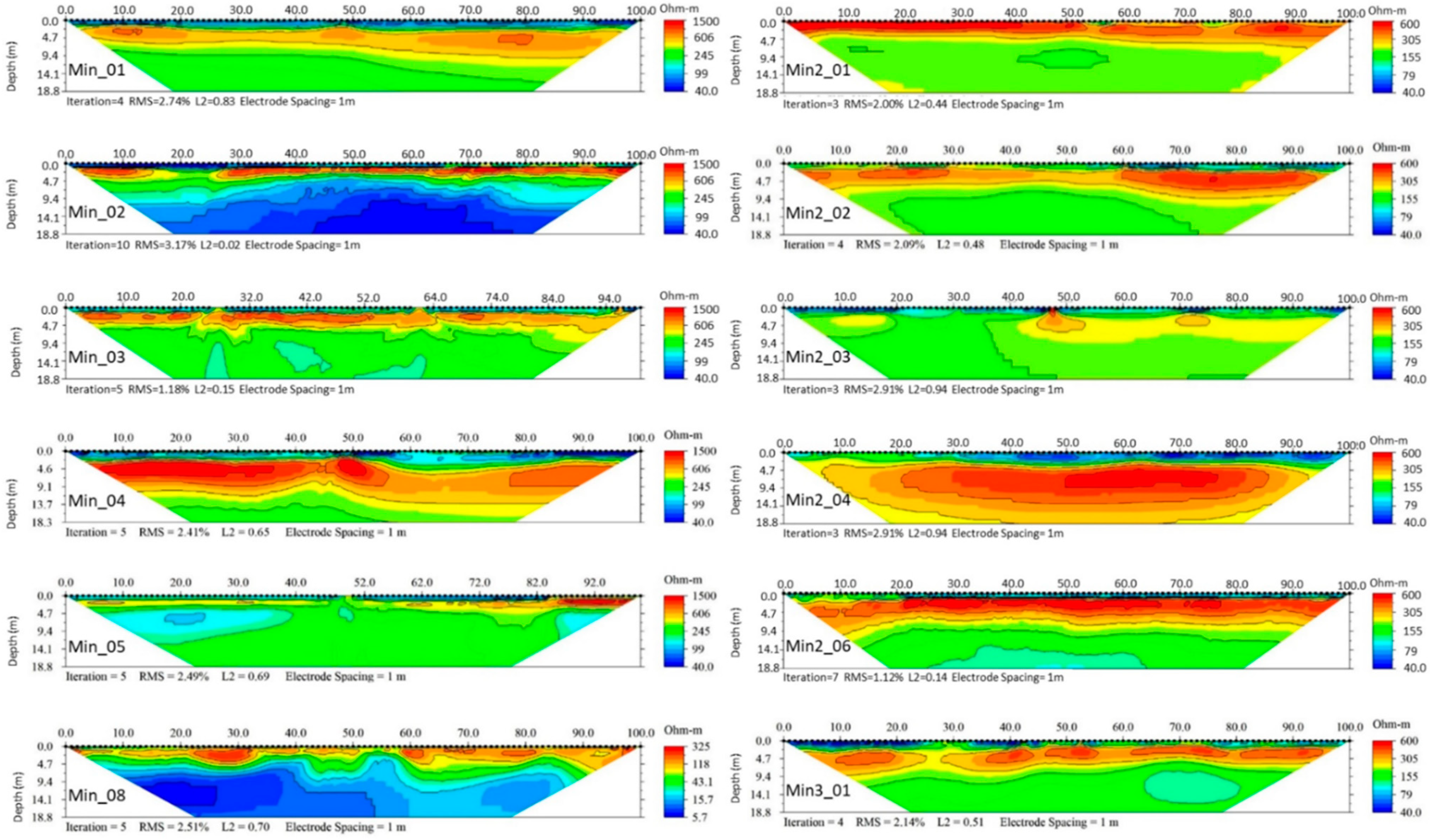
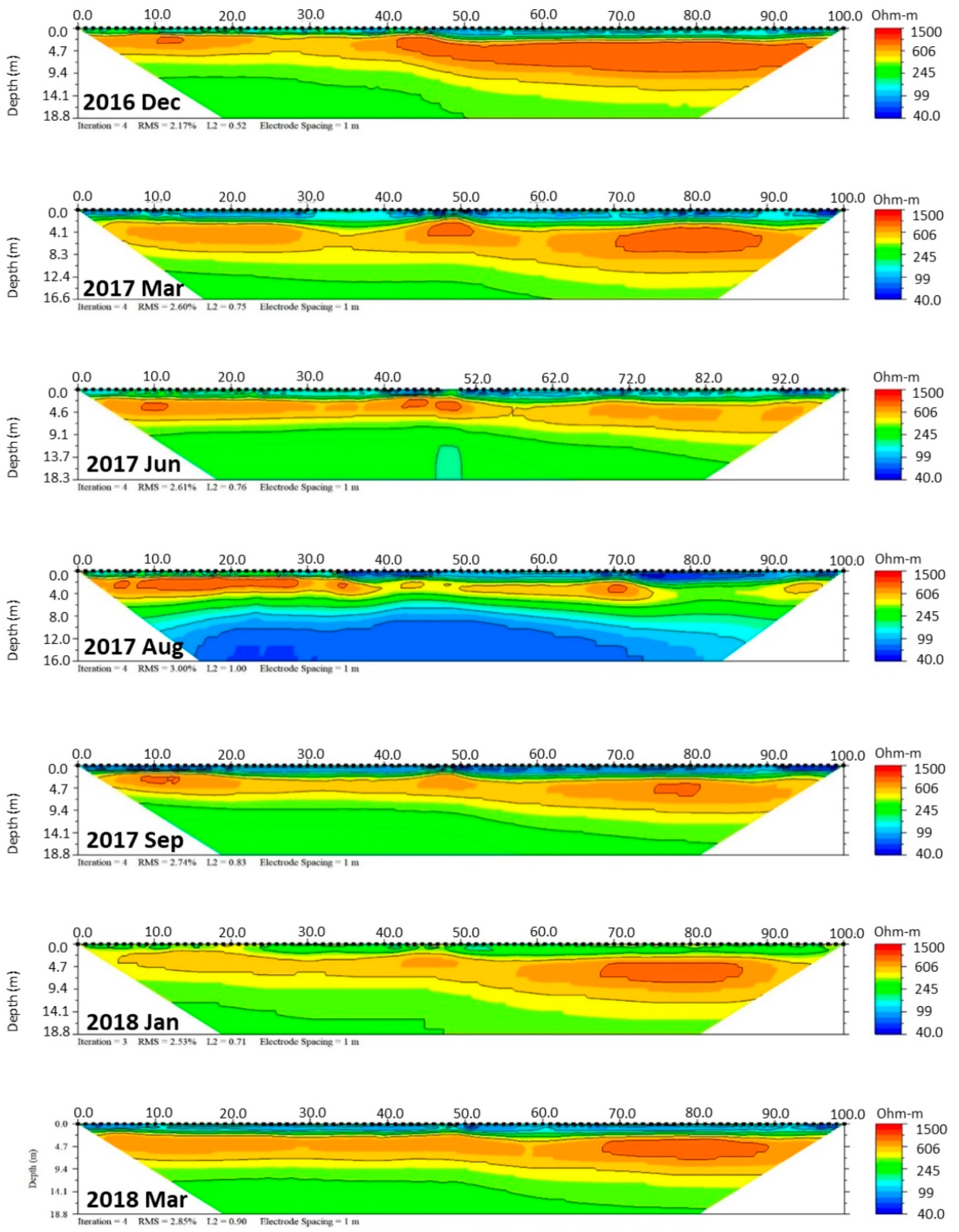
3.1. The Time-Lapse ERI Surveys

Except for the limited measurements in the pilot study, we started the Minzu Basin resistivity surveys in March of 2017. Figure 5 shows the inverted resistivity images for the surveys conducted at all sites in September of 2017, and Figure 6 shows the time-lapse resistivity images collected at the Min_01 site from December of 2016 to March of 2018. The Min_01 and Min_02 sites correspond to the survey lines that are closest to the Xinming observation well. Min_01 is located upstream of the Xinming well, while Min_02 is located downstream of the Xinming well, as shown in Figure 3. We found that a layer with resistivity from 20 to 100 Ohm-m lies between 1 m and 2 m below the ground surface in Min_01. The resistivity layer represents the soil layer of the rice field. Below the soil layer, the resistivity increases to over 400 Ohm-m. This area is between 2 m and 8 m below the soil layer. This relatively resistive layer may represent the unsaturated sand and gravel layer, which corresponds to the borehole logs in the Xinming well. Below 8 m depth, the resistivity value decreases from a peak of over 600 Ohm-m to a level between 330 and 230 Ohm-m. This change may reflect the effect of the increasing water content from the lower vadose zone to the saturation zone. Regarding changes in vertical resistivity, the inverted image of Min_02 presents a trend similar to that of Min_01. The resistivity value is between 40 Ohm-m and 70 Ohm-m for the shallow soil layer in the inverted image, and the region that is between 1 m and 5 m below the top layer consists of unsaturated sand and gravel with a resistivity between 400 Ohm-m and 1500 Ohm-m. Below 5 m depth, the resistivity decreases to less than 100 Ohm-m and exhibits the wetting feature of the sand and gravel. Among all resistivity survey lines, Min_08 is the northernmost one. Unlike the other survey lines, with an average resistivity that exceeds between 150 Ohm-m and 200 Ohm-m, the average resistivity of Min_08 is lower than 100 Ohm-m. The contact between the surface resistivity layer (resistivity higher than 100 Ohm-m) and the underlying conductivity layer (resistivity less than 50 Ohm-m) exhibits a wavy surface. The conductivity layer with a resistivity of less than 50 Ohm-m may imply that Min_08 has sediments containing more clay-like minerals than the other survey sites contain. Min3_01 and Min2_02 are the two southernmost sites among the survey lines. The two lines exhibit a resistivity pattern similar to that of Min_01. From the surface to a depth of about 2 m, soils have a resistivity of less than 80 Ohm-m in the inverted images of Min2_02 and Min3_01. The resistivity increases to over 300 Ohm-m in the vadose zone, and gradually decreases to about 100 Ohm-m in the saturated zone in both sites.

In the Minzu area, winter is the dry season and summer is the wet season. The inverted time-lapse images of Min_01 between December of 2016 and March of 2018 reveal the significant variations in the resistivity in the vadose zone between the dry and wet seasons. The region with a resistivity value higher than 500 Ohm-m mainly experiences this in December of 2016, and peak resistivity in the vadose zone can reach over 1500 Ohm-m. The resistivity region shrank from December of 2016 to August of 2017. This trend indicates that water content in the vadose zone increased owing to an increase in rainfall recharge. The resistivity region with a resistivity higher than 50 Ohm-m expanded from August of 2017 to January of 2018, because the rainfall decreased from the wet season into the dry season. The resistivity region in the inverted image for March of 2018 is slightly smaller than in January of 2018. The resistivity variations can be linked to changes in the vadose zone’s water content, according to Archie’s law in Equation (1). Hence, one may be able to estimate further the variation of water contents and the groundwater table with the inverted resistivity images collected in different seasons.

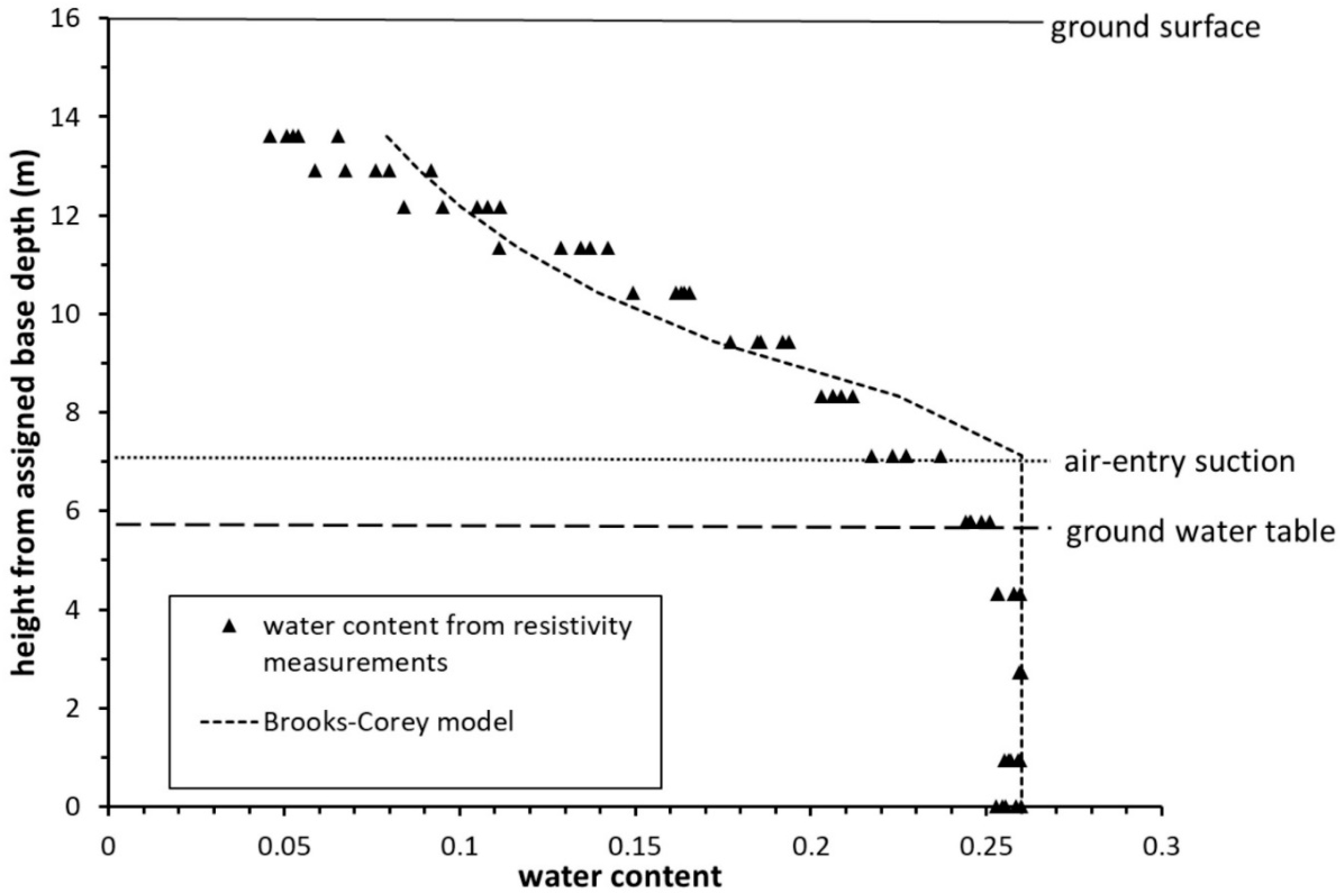
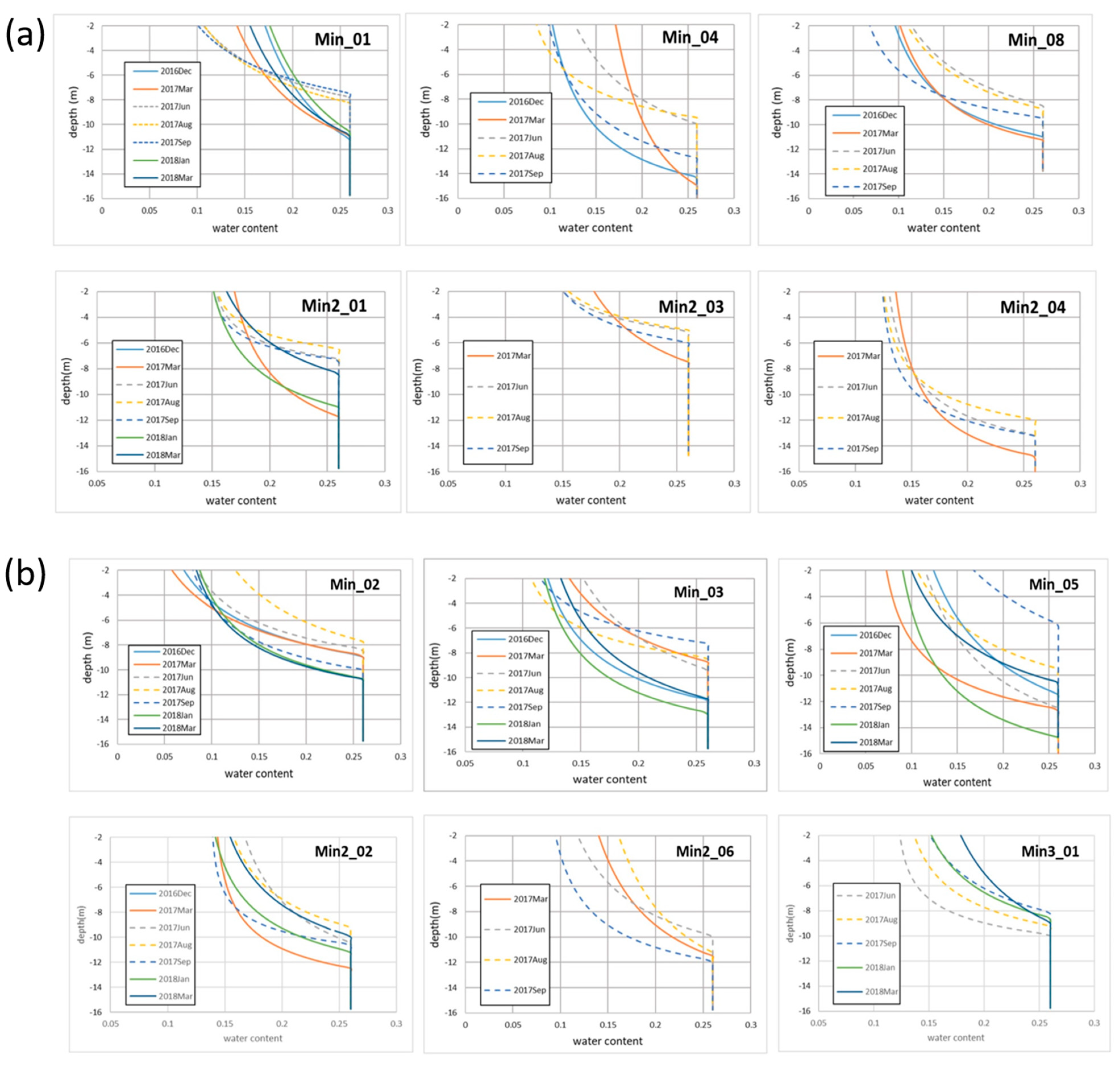
3.2. The Inverted Brooks-Corey Model

Using Equations (1)–(6), we were able to evaluate the parameters in the Brooks-Corey model for individual resistivity surveys. We selected five vertical profiles in the central part of each resistivity survey line for the estimation of water content. We used the entire observation period’s lowest water content as the residual water content, and assumed that the saturated water content would be equal to the average porosity, 0.26. Then, we could invert the air entry suction/heights from the base depth, $h_a$, and the Brooks-Corey parameter, $\lambda$, by minimizing the root mean square differences between the estimated and measured water content. We used the conjugated gradient methods with the EXCEL Solver to optimize the minimum object equation in the inversion.

Table 1. The estimated parameters of the Brooks-Corey model from the time-lapse resistivity surveys at the Min_01 survey site from 2016 to 2018. (${\theta }_s$ and ${\theta }_r$: the saturated and residual water content, $\lambda$: Brooks-Corey parameter, $h_a$: the air entry suction head).

Month	December 2016	March 2017	June 2017	August 2017	September 2017	January 2018	March 2018
λ	0.50	0.80	2.35	2.13	2.76	0.52	0.67
ha (m)	4.83	5.13	8.22	7.79	8.57	5.42	5.16
θs	0.26	0.26	0.26	0.26	0.26	0.26	0.26
θr	0.05	0.05	0.05	0.05	0.05	0.05	0.05

shows an example of the fitted parameters of the Brooks-Corey curve at the Min_01 site. The observed residual water content is about 0.05. Additionally, the fitted air entry heights vary from 4.8 m to 8.6 m, and are higher in the data sets for the June, August, and September wet season of 2017 than in the data sets for the observed months of the dry season. The Brooks-Corey parameters also vary from 0.5 m in the dry season to about 2.8 m in the wet season. Figure 7 shows the fitted Brooks-Corey curves for the time-lapse measurements at different survey sites.

Several sites—namely, Min_01, Min_04, Min_08, Min2_01, Min2_03, and Min2_04 (Figure 7a)—show that the fitted curves in the wet season have higher air entry heights than those in the dry season. Other sites—namely, Min_02, Min_03, Min_05, Min2_02, Min2_06, and Min3_01 (Figure 7b)—show that the air entry heights collected in some months during the dry season are higher than those collected during the wet season. In Figure 7b, we also observed that the air entry heights in March of 2017 are higher than those in the wet season at the upstream sites, Min_02, Min_03, and Min2_06. Min2_02 and Min3_01 are located downstream, and show no significant difference between their curves for the wet and dry seasons. Additionally, site Min_05, which is located near the northern foothill, exhibits a huge variation between the wet and dry season curves.

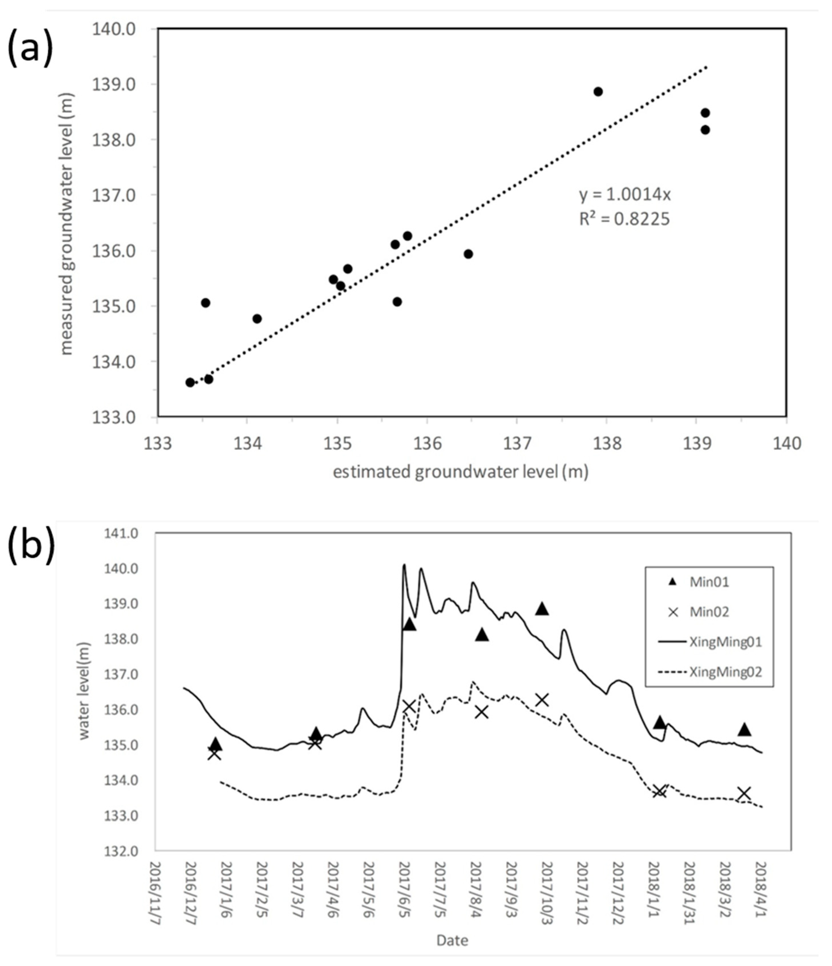
3.3. Estimation of Groundwater Levels

Equation (6) suggests that one may estimate the regional groundwater from the resistivity data after one corrects for differences between the estimated depth of the air entry suction and the measured groundwater depth from an observation well. The observed records of the Xinming well show two different groundwater levels. The levels are consistent, but the shallow one is about 1.5 m higher than the deep one. Because Min_01 is the closest survey line to the Xinming well, and may reflect shallow groundwater variations, we used the observed shallow groundwater level in the Xinming well and the measurements from Min_01 for the corrections. Regarding time-lapse measurements, the average difference between the observed shallow groundwater depth and the estimated air entry depth is about 1.7 m. Thus, we corrected the depth of the groundwater table by subtracting the average difference from the estimated air entry depths. By considering the ground levels, we estimated the groundwater levels from the resistivity measurements. Figure 8a shows the correlation between the estimated and observed groundwater levels in both Min_01 and Min_02. With Min_02, which is located near the Xinming well in the downstream area, we tested whether or not the correction value of 1.7 m, estimated from Min_01, was still applicable for Min_02. The slope of the regression line is about 1, and the coefficient of determination R² is about 0.82. Thus, there is good agreement between the estimated and observed groundwater levels. In addition, Figure 8b presents two important sets of information: first, the estimated groundwater levels at the Min_01 and Min_02 sites, and second, the variation in the observed groundwater levels in the shallow and deep observation wells. The estimated groundwater levels at Min_01 are consistent with the measurements in the shallow observation well. Interestingly, we observed that the estimated groundwater levels at Min_02 were consistent with the observed groundwater levels in the shallow well before March of 2017, yet the estimated groundwater levels agree better with those measured in the deep well after Jun of 2017. The double groundwater levels observed from the Min_01 site, Min_02 site, and Xinming well in the unconfined aquifer next to the river channel may suggest an interaction between the perched river subsurface flow and the regional groundwater base flow, e.g., [24].

Table 2. The ground levels and estimated groundwater levels were collected at survey sites during December of 2016 and March of 2018.

Survey Line	X-Corr (TM97)	Y-Corr (TM97)	Ground Level (m)	Groundwater Level (m)
				December 2016	March 2017	June 2017	August 2017	September 2017	January 2018	March 2018
Min_01	219,425.6	2,634,326.9	148	135.1	135.4	138.5	138.2	138.9	135.7	135.5
Min_02	219,009.2	2,634,177.1	146.2	134.8	136.1	136.2	136.8	134.5	133.8	133.7
Min_03	218,467.3	2,634,382.7	143.5	130.0	133.1	132.4	133.4	134.6	129.0	130.1
Min_04	219,170.5	2,634,928.7	150	134.0	133.3	138.3	138.8	135.5
Min_05	218,182.1	2,634,650.5	142	128.9	127.7	127.8	130.8	134.2	125.6	129.8
Min_08	218,874.6	2,635,552.2	149	137.1	136.8	139.6	139.3	138.6
Min2_01	217,203.4	2,633,563.7	135		121.6	126.1	126.9	126.0	122.3	124.9
Min2_02	216,878.5	2,633,495.5	131.2		117.0	119.1	120.3	118.9	118.3	119.6
Min2_03	217,496.7	2,634,252.7	135		125.8	128.2	128.3	127.3
Min2_04	218,269.1	2,633,408.5	137		120.5	122.1	123.4	122.1
Min2_06	218,851.7	2,634,480.1	145.5		132.3	133.9	132.6	131.9
Min3_01	217,554.3	2,632,769.4	129			117.4	118.1	119.2	118.7	118.4

lists the corrected groundwater levels measured at different survey sites during the observation period between 2016 and 2018.

Figure 9a–d show the distribution of corrected groundwater levels for March, June, August, and September of 2017 in the study area. In general, the groundwater flow follows a trend from upstream to downstream, with a higher hydraulic gradient near the river channel than the area away from the main channel. The area near Min_01 and Min_02 show a pattern suggesting that the groundwater is recharged from the river channel. Yet, in the downstream area near Min2_05 and Min3_01, the groundwater discharges into the aquifer under the river channel. The groundwater level in March of 2017 was about 3 m lower than the groundwater levels in June, August, and September of 2017. The groundwater level difference between March of 2017 and August of 2017 is about 2 m in the upstream area near Min_01 and about 4 m in the downstream area near Min2_04.

4. Discussion

Besides the seasonal variation in groundwater levels, it is necessary to know the water storage capacity of the regions for potential groundwater reservoirs. The specific yield, $S_y$, which denotes the ratio of water volume that can be drained from the total volume of rock or soils, is the most important hydrogeological parameter in the assessment of the storage potential for the groundwater reservoirs.

We can obtain the theoretical specific yield, $S_y$, by calculating the difference between the saturated water content, ${\theta }_s$, and the residual water content, ${\theta }_d$:

$$S_y={\theta }_s-{\theta }_r.$$

(7)

Table 3. The estimated theoretical specific yields and specific yield capacities collected at survey sites during December of 2016 and March of 2018.

Survey Line	Theoretical Specific Yield	Specific Yield Capacity							Maximum	Average
		December 2016	March 2017	June 2017	August 2017	September 2017	January 2018	March 2018
Min_01	0.21	0.06	0.09	0.12	0.14	0.12	0.06	0.08	0.14	0.09
Min_02	0.21	0.13	0.14	0.14	0.10	0.16	0.13	0.15	0.16	0.13
Min_03	0.17	0.11	0.08	0.08	0.12	0.12	0.09	0.07	0.12	0.10
Min_04	0.19	0.12	0.06	0.10	0.14	0.12			0.14	0.11
Min_05	0.20	0.10	0.15	0.11	0.12	0.07	0.13	0.12	0.15	0.11
Min_08	0.22	0.13	0.12	0.11	0.11	0.15			0.15	0.12
Min2_01	0.11		0.06	0.09	0.09	0.09	0.08	0.07	0.09	0.08
Min2_02	0.12		0.08	0.07	0.08	0.08	0.08	0.07	0.08	0.08
Min2_03	0.13		0.06	0.09	0.09	0.09			0.09	0.08
Min2_04	0.14		0.10	0.11	0.11	0.11			0.11	0.11
Min2_06	0.19		0.09	0.11	0.07	0.13			0.13	0.10
Min3_01	0.14			0.11	0.10	0.08	0.08	0.06	0.11	0.08

lists the estimated theoretical specific yield, $S_y,$ at different survey sites, and Figure 10a shows the distribution of the theoretical specific yield in the study area. In general, the theoretical specific yields are higher in the northeastern part of the basin than those in the southwestern part of the basin. The highest specific yield is about 0.21 at the Min_01 and Min_02 sites, and the lowest one is 0.11 at Min2_01. The trend of the theoretical specific yields indicates the sediment distribution pattern from the upstream to the downstream parts of the Choushui River in the Minzu Basin. In addition, we observed that specific yields in the area near Min_03, Min2_06, and Min_04 are lower than the corresponding yields in nearby sites.

The theoretical specific yield, $S_y,$ refers to the maximum groundwater volume ratio that can be yielded from or stored in an unconfined aquifer if the aquifer can be totally dried out. However, in natural conditions, groundwater volume ratios that can be pumped from or stored in a sediment/rock matrix cannot reach a specific yield because of capillary fringes in the vadose zone. Thus, in the current study, we define the specific yield capacity, $S_c$, as the natural specific yield corresponding to the capillary fringes in the vadose zone. With the Brooks-Corey model in Equation (5), one should be able to calculate $S_c$ as:

$$S_c=\frac{1}{H}{{\displaystyle \int }}_0^H\left({\theta }_s-\theta \left(h\right)\right)dh\cong \frac{1}{H}{{\displaystyle \sum }}_0^H\left({\theta }_s-\theta \left(h\right)\right)\Delta h,$$

(8)

where H is the depth of the groundwater, $\theta \left(h\right)$ is the volumetric water content at a different depth, $h$, and $\Delta h$ is the incremental depth. Table 3 lists our calculation of $S_c$ for different survey sites in different months during the study period. The specific yield capacity at different sites varies between 0.06 and 0.16 in the study area. With the exception of the Min_05, Min_08, and Min2_02 sites, most sites generally have a higher $S_c$ value in the wet season (June, August, and September) than in the dry season. The Min2_02 site exhibits almost the same $S_c$ value during the wet and dry seasons. Min_08 exhibits a lower $S_{\mathrm{c}}$ value in June and August than in September, when the site reaches its maximum value, 0.15. Unlike the other sites, Min_05 exhibits higher $S_c$ levels in the dry season than in the wet season. The fact that the specific yield capacity varies between the wet and dry seasons may indicate the hysteresis behavior of the drying and wetting curves of the Brooks-Corey model.

Figure 10b shows the distribution of the averages, and Figure 10c shows the maximum specific yield capacities. Although the specific yield capacities vary during the research period for most of the survey sites, the average and maximum specific yield capacities have a distribution pattern similar to that of the theoretical specific yields. However, the estimated values for the maximum and average specific yield capacities are, respectively, only about 72% and 60% of the theoretical specific yields. The specific yield estimated from the in situ pumping test in the Xinming well is about 0.157, and is close to the maximum specific yield capacities of Min_01 ($S_c=0.14$) and Min_02 ($S_c=0.16$), as shown in Table 3. These findings suggest that the specific yield capacity is consistent with the value estimated from the in situ pumping test, and is only three quarters to two thirds of the theoretical specific yield. When evaluating potential groundwater reservoirs, one should take this difference into account. The aquifer area of the Minzu Basin is about 69.8 km². If we use the maximum $S_c$ for the estimation, the water volume that can be stored in the unconfined aquifer in the Minzu Basin is about 8,716,000 m³ for one meter of increase in the groundwater level. The estimated value is similar to the estimation by Hsiao and Chang [25], who conducted time-lapse gravity measurements.

The spatial distribution of the hydrogeological parameters of the unconsolidated sediments is often subject to the deposition patterns of river systems, and it is important to consider when planning the artificial recharge surface ponds effectively for the potential groundwater reservoirs. In theory, the specific yields should decrease from upstream to downstream, with the contours appearing to be slightly concave as one moves further upstream along the Choushui River, since the river channels consists of mainly the coarser materials, more so than the overbank deposits. Yet the pattern associated with the contours of specific yields is not only concave along the river, but also along the direction from Min_05 to Min_08. In addition, the pattern exhibits a lateral variation in the direction perpendicular to the river, with a lower specific yield at Min_03, and is not consistent with the current channel distribution patterns. We tried to overlap the specific yield contours with the old river channels that were mapped in 1904, as shown in Figure 11. Unlike today’s Choushui River channel, which was artificially modified, the old map shows that the natural Choushui River branched into two channels 130 years ago. Additionally, an area with low specific yields is located between the two main channels. The difference in groundwater levels between the wet and dry seasons also suggests a greater change at Min_03, which exhibits lower specific yields than the neighboring site in Figure 11. The findings from the old map help to explain the special contour pattern of the specific yields. The “ancient” river channels show higher specific yields than their neighboring areas. Additionally, the old map that presents the nature system before the artificial modification of channels should be taken into account when planning the surface recharge activities for the groundwater reservoirs.

5. Conclusions

To evaluate a potential groundwater reservoir, we used time-lapse resistivity measurements collected at 12 sites in the Minzu Basin. Thus, we specifically estimated both groundwater levels and specific yields for various months from 2016 to 2018. Using Archie’s law, we converted the time-lapse resistivity measurements into water content values. We then estimated the groundwater levels and the specific yields with the Brooks-Corey (BC) model and water content vertical profiles.

The contour maps of the time-lapse groundwater levels show that the groundwater flowing downstream had a higher hydraulic gradient near the river channel than in the area away from the main channel. On average, the groundwater level in the dry season (i.e., from December to March) is about 3 m lower than in June, August, and September. From the BC model, we also estimated the theoretical specific yields that might provide crucial information about the potential groundwater reservoir. The difference between the residual and saturated water content of the fitted BC model is key to obtaining the theoretical specific yield at different survey sites. Additionally, using the BC model, we calculated specific yield capacities, which represent the nature of the storage capacity in the aquifer, across several months. The estimated theoretical specific yields for both the Min_01 and Min_02 sites are 0.21. However, the estimated maximum specific yield capacities for the Min_01 and Min_02 sites are about 0.14 and 0.16, respectively, and are consistent with both the specific yields estimated from the in situ pumping test in the Xinming observation well (S_y = 0.157) and the maximum specific yield capacities estimated from the resistivity measurements. The findings suggest that the specific yield capacities are consistent with the values estimated from the in situ pumping tests, and are only three quarters to two thirds of the theoretical specific yields. Using the estimation from the maximum specific yield capacities, there is about 8,716,000 m³ of water that can be stored in the unconfined aquifer in the Minzu Basin if the groundwater level is increased by one meter.

The distribution pattern of the specific yield contours reveals the natural river channel pattern shown in the old map completed in 1904, since the current river channel has been artificially modified over the past 100 years. The natural Choushui River branched into two channels in the Minzu Basin on the 1904 map before the human modification. The “ancient” river channels thus show higher specific yields than their neighboring areas. Our study shows that resistivity surveys provide good estimations of hydraulic parameters for preliminary evaluations, especially in an area in which few observation wells are available.

References

1. Michot, D.; Benderitter, Y.; Dorigny, A.; Nicoullaud, B.; King, D.; Tabbagh, A. Spatial and temporal monitoring of soil water content with an irrigated corn crop cover using surface electrical resistivity tomography. Water Resour. Res. 2003, 39, 1138. [Google Scholar] [CrossRef]
2. Berthold, S.; Bentley, L.R.; Hayashi, M. Integrated hydrogeological and geophysical study of depression-focused groundwater recharge in the Canadian prairies. Water Resour. Res. 2004, 40, W06505. [Google Scholar] [CrossRef] [Green Version]
3. Rayner, S.F.; Bentley, L.R.; Allen, D.M. Constraining Aquifer Architecture with Electrical Resistivity Imaging in a Fractured Hydrogeological Setting. J. Environ. Eng. Geophys. 2007, 12, 323–335. [Google Scholar] [CrossRef]
4. Frohlich, R.K.; Kelly, W.E. Estimates of specific yield with the geoelectric resistivity method in glacial aquifers. J. Hydrol. 1988, 97, 33–44. [Google Scholar] [CrossRef]
5. Dietrich, S.; Carrera, J.; Weinzettel, P.; Sierra, L. Estimation of Specific Yield and its Variability by Electrical Resistivity Tomography. Water Resour. Res. 2018, 54, 8653–8673. [Google Scholar] [CrossRef]
6. Chang, P.-Y.; Chang, L.-C.; Hsu, S.-Y.; Tsai, J.-P.; Chen, W.-F. Estimating the hydrogeological parameters of an unconfined aquifer with the time-lapse resistivity-imaging method during pumping tests: Case studies at the Pengtsuo and Dajou sites, Taiwan. J. Appl. Geophys. 2017, 144, 134–143. [Google Scholar] [CrossRef]
7. Wang, S.-J.; Lee, C.-H.; Yeh, C.-F.; Choo, Y.; Tseng, H.-W. Evaluation of Climate Change Impact on Groundwater Recharge in Groundwater Regions in Taiwan. Water 2021, 13, 1153. [Google Scholar] [CrossRef]
8. Huang, W.-C.; Chiang, Y.; Wu, R.-Y.; Lee, J.-L.; Lin, S.-H. The impact of climate change on rainfall frequency in Taiwan. Terr. Atmos. Ocean. Sci. 2011, 23, 553. [Google Scholar] [CrossRef] [Green Version]
9. Archie, G.E. The electrical resistivity log as an aid in determining some reservoir characteristics. Pet. Trans. AIME 1942, 146, 54–62. [Google Scholar] [CrossRef]
10. Dachnov, V. Interpretazija resultatov geofiziceskichissledovanij razrezov skavzin. Izdat. Gostoptechizdat 1962, 2, 547. [Google Scholar]
11. Zhou, B. Electrical Resistivity Tomography: A Subsurface-Imaging Technique, in Applied Geophysics with Case Studies on Environmental, Exploration and Engineering Geophysics; IntechOpen: London, UK, 2018. [Google Scholar]
12. Lippmann, E. Four-Point Light Hp Technical Data and Operating Instructions Ver. 3.37.; Lipmann Geophysikalische Messgeräte: Schaufling, Germany, 2005. [Google Scholar]
13. Dahlin, T.; Zhou, B. A numerical comparison of 2D resistivity imaging with 10 electrode arrays. Geophys. Prospect. 2004, 52, 379–398. [Google Scholar] [CrossRef] [Green Version]
14. Tamssar, A.H. An Evaluation of the Suitability of Different Electrode Arrays for Geohydrological Studies in Karoo Rocks Using Electrical Resistivity Tomography; University of the Free State: Bloemfontein, South Africa, 2013. [Google Scholar]
15. AGI. Instruction Manual for EarthImager 2D ver. 2.3.0.; Advanced Geosciences, Inc: Austin, TX, USA, 2006. [Google Scholar]
16. Yang, X.; Lagmanson, M.B. Planning resistivity surveys using numerical simulations. In Proceedings of the 16th EEGS Symposium on the Application of Geophysics to Engineering and Environmental Problems, European Association of Geoscientists & Engineers, San Antonio, TX, USA, 6–10 April 2003. [Google Scholar]
17. Yang, X.; LaBrecque, D.J. Stochastic inversion of 3D ERT data. In Symposium on the Application of Geophysics to Engineering and Environmental Problems 1998; Society of Exploration Geophysicists: Chicago, IL, USA, 1998. [Google Scholar]
18. Sharma, S.; Verma, G. Inversion of Electrical Resistivity Data: A Review. World Acad. Sci. Eng. Technol. Int. J. Environ. Chem. Ecol. Geol. Geophys. Eng. 2015, 9, 400–406. [Google Scholar]
19. Novák, V.; Hlaváčiková, H. Soil-Water Retention Curve, in Applied Soil Hydrology; Springer International Publishing: Cham, Switzerland, 2019; pp. 77–96. [Google Scholar]
20. Fredlund, D.G.; Sheng, D.; Zhao, J. Estimation of soil suction from the soil-water characteristic curve. Can. Geotech. J. 2011, 48, 186–198. [Google Scholar] [CrossRef]
21. Krahn, J.; Fredlund, D. On total, matric and osmotic suction. Soil Sci. 1972, 114, 339–348. [Google Scholar] [CrossRef]
22. Brooks, R.; Corey, A. Hydraulic Properties of Porous Media, in Hydrology Papers; Colorado State University: Ft. Collins, CO, USA, 1964. [Google Scholar]
23. Van Genuchten, M.T. A Closed Form Equation for Predicting the Hydraulic Conductivity of Unsaturated Soils. Soil Sci. Soc. Am. J. 1980, 44, 892–898. [Google Scholar] [CrossRef] [Green Version]
24. Niswonger, R.G.; Fogg, G.E. Influence of perched groundwater on base flow. Water Resour. Res. 2008, 44, W03405. [Google Scholar] [CrossRef] [Green Version]
25. Hsiao, Y.-S.; Chang, J.-C.; Yang, R.-J.; Tseng, T.-P. Estimating the specific yield in an unconfined aquifer using the gravimetric method: A case study in the Zhoushui River alluvial fan. J. Chin. Inst. Eng. 2021, 44, 820–830. [Google Scholar] [CrossRef]
Figure 1. The geographic map of the Minzu Basin (located in the area enclosed by the black dotted line) and our study area (the red rectangular area). The red star represents the only observation well, the Xinming well, in the basin.
Water 14 00420 g001
Figure 2. The borehole logs (left) and resistivity logging (right) records of the Xinming observation well. The 16” and 64” normal logging, which represent the domain near the borehole and at the far side of the borehole, respectively, were registered at an interval of 5 cm.
Water 14 00420 g002
Figure 3. The distribution of the resistivity survey lines in the Minzu Basin. The red star represents the location of the Xinming observation well.
Water 14 00420 g003
Figure 4. The selected vertical profiles of the normalized volumetric water content from resistivity measurements from the Min_01 survey line. The dashed curve indicates the fitted Brooks-Corey model regarding the relationship between normalized volumetric water content and height from a presumed baseline. The dotted line indicates the air entry suction and the dashed level line represents the observed groundwater table in the nearby Xinming observation well.
Water 14 00420 g004
Figure 5. The inverted resistivity images of the survey lines in the Minzu Basin collected in September of 2017. Note that the scales of resistivity for Min_08, Min2_02, Min2_03, Min2_04, and Min3_01 differ from the scales of other sites. These differences help to show the variation in resistivity clearly.
Water 14 00420 g005
Figure 6. The time-lapse resistivity images collected at the Min_01 site during the period from December of 2016 to March of 2018.
Water 14 00420 g006
Figure 7. The fitted Brooks-Corey model for different months at the survey sites in the Minzu Basin. The dotted curves indicate the models for the months in the wet season, and the solid curves are the fitted models for the months in the dry season. (a) The sites with fitted curves in the wet seasons have higher air entry heights than those in the dry seasons. (b) The sites with some fitted curves in the dry seasons have higher air entry heights than those in the wet seasons.
Water 14 00420 g007
Figure 8. (a) The correlation between the estimated and observed groundwater levels in the Min_01 and Min_02 sites. The solid line is the linear regression line with a slope of about 1 and an R2 of about 0.82. (b) A comparison of the estimated groundwater levels at the Min_01 and Min_02 sites and the observed groundwater levels in the shallow (solid curve) and deep (dotted curve) Xinming wells.
Water 14 00420 g008
Figure 9. (a) The distribution of corrected groundwater levels in (a) March (the dry season), (b) June (the intermediate season), (c) August (the wet season), and (d) September (the wet season) of 2017.
Water 14 00420 g009
Figure 10. The distribution of (a) the theoretical specific yield, (b) the averaged specific yield capacity, and (c) the maximum specific yield capacity during the study period in the study area.
Water 14 00420 g010
Figure 11. Left: The old river channel recorded in 1904, labeled with orange color, overlapped onto the present-day maps and contours of the maximum specific yield capacity. Right: The difference between water levels in August and in March of 2017.
Water 14 00420 g011