Article

Optimum Multiparameter Analysis of Water Mass Structure off Western Guangdong during Spring Monsoon Transition

1
School of Marine Sciences, Sun Yat-sen University, Zhuhai 519082, China
2
Southern Laboratory of Ocean Science and Engineering (Guangdong, Zhuhai), Zhuhai 519000, China
3
Guangdong Provincial Key Laboratory of Marine Resources and Coastal Engineering, Guangzhou 510275, China
4
Pearl River Estuary Marine Ecosystem Research Station, Ministry of Education, Zhuhai 519000, China
*
Author to whom correspondence should be addressed.
Water 2022, 14(3), 375; https://doi.org/10.3390/w14030375
Submission received: 3 December 2021 / Revised: 14 January 2022 / Accepted: 19 January 2022 / Published: 26 January 2022
(This article belongs to the Special Issue River Restoration and Morphodynamics)

Abstract

:
Water masses and their variability play vital roles in regulating ocean circulation, material exchanges and biogeochemical processes. However, there is still a lack of quantitative analysis of water mass distributions in coastal waters of the South China Sea. Here, two oceanographic cruise observations in April and May 2016 are used to quantify water mass distributions, pathways and mixture, and their intraseasonal variability off western Guangdong during the spring monsoon transition. Temperature and salinity observations qualitatively reveal that there are three types of water masses: the Pearl River diluted water (PRDW, salinity (S) = 22 psu, potential temperature (θ) = 25 °C), the South China Sea surface water (SCSSW, S = 34 psu, θ = 28 °C) and the South China Sea subsurface water mass (SCSSUW, S = 34.5 psu, θ = 17 °C). Their relative contributions and intraseasonal variability are quantified using the Optimum Multiparameter (OMP) method. The PRDW is largely confined to the upper 10 m layer in shallow nearshore waters (depths < 30 m), with a maximum contribution >90% near the Pearl River Estuary. The SCSSW mainly dominates the rest of the surface layer above 20 m, with a contribution >50% in offshore regions. The layer below 20 m is primarily composed of ~60% SCSSW and ~40% SCSSUW. A comparison between the two different observations suggests that the PRDW tends to expand southwestward and the SCSSUW spreads offshore, whereas the SCSSW moves landward and is situated underneath the surface fresh PRDW. These characteristics are very likely associated with the wind transition from weak southeasterly in April to strong northeasterly in May, which enhances the southwestward coastal current and the onshore surface Ekman transport from offshore waters.

1. Introduction

Water masses are ubiquitous in oceans. They are defined as water bodies with similar properties and common formation history, and have a measurable extent in the vertical and horizontal directions [1,2,3,4]. Water mass distributions and their variations play a significant role in modulating global thermohaline circulation, heat/freshwater budget and climate change [5,6,7,8]. In addition, diffusion and mixing associated with water mass exert a great impact on ecological environment variability through altering local temperature, salinity, dissolved oxygen and nutrient distributions [9].
The South China Sea (SCS) is a unique, semi-enclosed marginal sea in the western Pacific Ocean, with a maximum depth > 3 km [10]. A pronounced feature of its bathymetry is the wide, shallow continental shelf in the northern SCS (NSCS) where the isobaths are approximately in parallel with the coastline. The shelf connects with the third largest river of China, called the Pearl River (PR), through the Pearl River Estuary (PRE) (Figure 1a). The climate in the NSCS is primarily dominated by the East Asian Monsoon, with strong northeasterly winds in winter, weak southwesterly winds in summer, and transitions in both spring and autumn [11,12,13]. The downwelling-favorable winter winds induce the fresh, cold PR plume along the western side of the PRE, while the upwelling-favorable summer winds lead to the appearance of the fresh plume along the eastern side [14,15]. Under the influence of the complex topography, monsoon, and Kuroshio intrusion, the upper ocean circulation also presents distinct features. There is a southwestward slope current deeper than 200 m throughout the year, a northeastward SCS warm current over the shelf, and a seasonally varying coastal current along the Guangdong coast (i.e., Guangdong Coastal Current). The coastal current flows southwestward during both summer and winter, and sporadically reverses northeastward when the southwesterly wind is strong [16]. All these processes could significantly modify the spatial pattern and variability of the NSCS water masses.
Great efforts have been made to investigate the spatiotemporal variability of water masses in the NSCS based on hydrographic observations since 1980s [17,18,19]. Using the temperature–salinity (T-S) diagram, Li et al. [20] identified the Kuroshio and SCS water in the upper layer (<400 m) of the northeastern SCS. Tian and Wei [21] divided the SCS-basin water masses into four types in the vertical direction: surface water, subsurface water, intermediate water and deep water. Using the cluster analysis, Cheng et al. [22] categorized the NSCS summer water masses into five types: coastal mixing water, surface water, subsurface water, intermediate water and deep water. By combining the cluster analysis with the T-S diagram, Zhu et al. [23] classified the upper layer (<300 m) water of the NSCS into six water masses: diluted water, surface water, SCS subsurface water, Pacific subsurface water, surface–subsurface mixed water and subsurface–intermediate mixed water. Based on the potential density–potential spicity (sigma-pi) diagram, Gao et al. [24] distinguished the NSCS spring water masses into thirteen types: PR diluted water, SCS surface water, west Pacific Ocean (WPO) surface water, SCS surface–subsurface mixed water, WPO surface–subsurface mixed water, SCS subsurface water, WPO subsurface water, SCS subsurface–intermediate water, WPO subsurface–intermediate mixed water, SCS intermediate water, WPO intermediate water, SCS deep water, and WPO deep water.
While the water mass compositions in the NSCS have been well documented, very few observational studies have been made to quantify the contributions of each water mass. One exception is to determine the composition and proportion of the upper 55 m water masses in the NSCS, as conducted by Li et al. [25]. They found that the surface water between the 200- and 2000-meter isobaths is composed of SCS surface water, Kuroshio water and shelf water. The contribution of the SCS surface water is about 60–100%. Their study “helps to fill a conspicuous void” of the quantitative water mass analysis in the NSCS. We note however that their study focused on the northeastern SCS slope, and their study period was limited to the summer condition. To the best of the present authors’ knowledge, the contributions of different water masses in coastal waters of the SCS have not been quantified yet. The characteristics of the water mass contributions at an intraseasonal time scale and the role of the variable winds in the water mass variability, remain to be resolved.
In this study, in situ hydrographic observations from two oceanographic cruises off western Guangdong during April and May 2016 are analyzed together with the corresponding surface winds and numerical currents. We attempt to accomplish two objectives: (1) to quantify contributions of different water masses during the spring monsoon transition based on the optimum multiparameter analysis, and (2) to investigate their intraseasonal variability.

2. Data and Methods

2.1. Data

The study area covers 110.8° E–115° E in longitude and 20.5° N–22.5° N in latitude off western Guangdong in the NSCS. Two cruises during 12–18 April and 13–20 May of 2016 were conducted onboard the R/V Zhanjiang Kediao to collect hydrographic data from the SeaBird 911 CTD (conductivity–temperature–depth) recorder. A total of 86 casts in April and 88 casts in May were made at the sampling stations with depths shallower than 60 m (Figure 1b).
There was no direct measurement of three-dimensional currents over the vast area. To illustrate the water mass variability, we used the daily mean currents with a horizontal resolution of 1/12° from OMGOAFS (Operational Mercator global ocean analysis and forecast system) (http://marine.copernicus.eu/, accessed on 31 May 2021). The OMGOAFS is based on the Nucleus for European Modelling of the Ocean (NEMO) and the Système d’Assimilation Mercator (SAM) data assimilation system. It is driven by atmospheric fields from the European Centre for Medium-Range Weather Forecasts (ECMWF), and assimilates various satellite and in situ observations. We also obtained the Cross-Calibrated Multi-Platform (CCMP) gridded surface winds from Remote Sensing Systems (https://www.remss.com/measurements/ccmp/, accessed on 20 September 2020).

2.2. Optimum Multiparameter Method

The Optimum Multiparameter (OMP) method was originally developed by Tomczak [26]. It is an extension of classical temperature–salinity analysis to quantitatively analyze water masses. Its central idea is to determine the quantitative mixing ratios of different source water types (SWTs) from quasi-conservative properties (e.g., potential temperature and salinity) though solving a linear system of mixing equations. The method has been successfully applied to quantitatively analyze the distribution and movement of the water masses in various regions around the world, including the Eastern Indian Ocean [27], the Ross Sea [28], the Sargasso Sea [29], the Southern Ocean [30], the Southern Drake Passage [31], the Coral Sea [32], the Faroe–Shetland Channel [33] and the East China Sea [34].
In this study, two properties of each SWT (potential temperature θ and salinity S) are used, and the OMP method solves the following linear system of conservative-mixing equations:
{ X 1 · θ 1 + X 2 · θ 2 + X 3 · θ 3 = θ o b s + R θ X 1 · S 1 + X 2 · S 2 + X 3 · S 3 = S o b s + R S X 1 + X 2 + X 3 = 1 + R M
where X i is the contribution (%) of each S W T i , θ i and S i represent the predetermined potential temperatures and salinities of the SWTs, “obs” denotes observed properties, R θ , R S , and R M are residuals. The last equation refers to mass conservation. The above system can be written in a matrix form:
G X   =   d   +   R
where G is the SWT definition matrix, X is the unknown solution vector of the SWT fractions, d is the observation vector, and R is the residual error [31,32,35]. More detailed description of the OMP method and the corresponding Matlab codes are publicly available at https://omp.geomar.de/, accessed on 20 September 2020.
To concisely display the analyzed results, Figures in this paper are almost all plotted by MATLAB software with M_Map package, while the horizontal distributions of different water mass contributions are produced by Ocean Data View (ODV) and MATLAB software.

3. Results and Discussion

3.1. Definition of Source Water Types
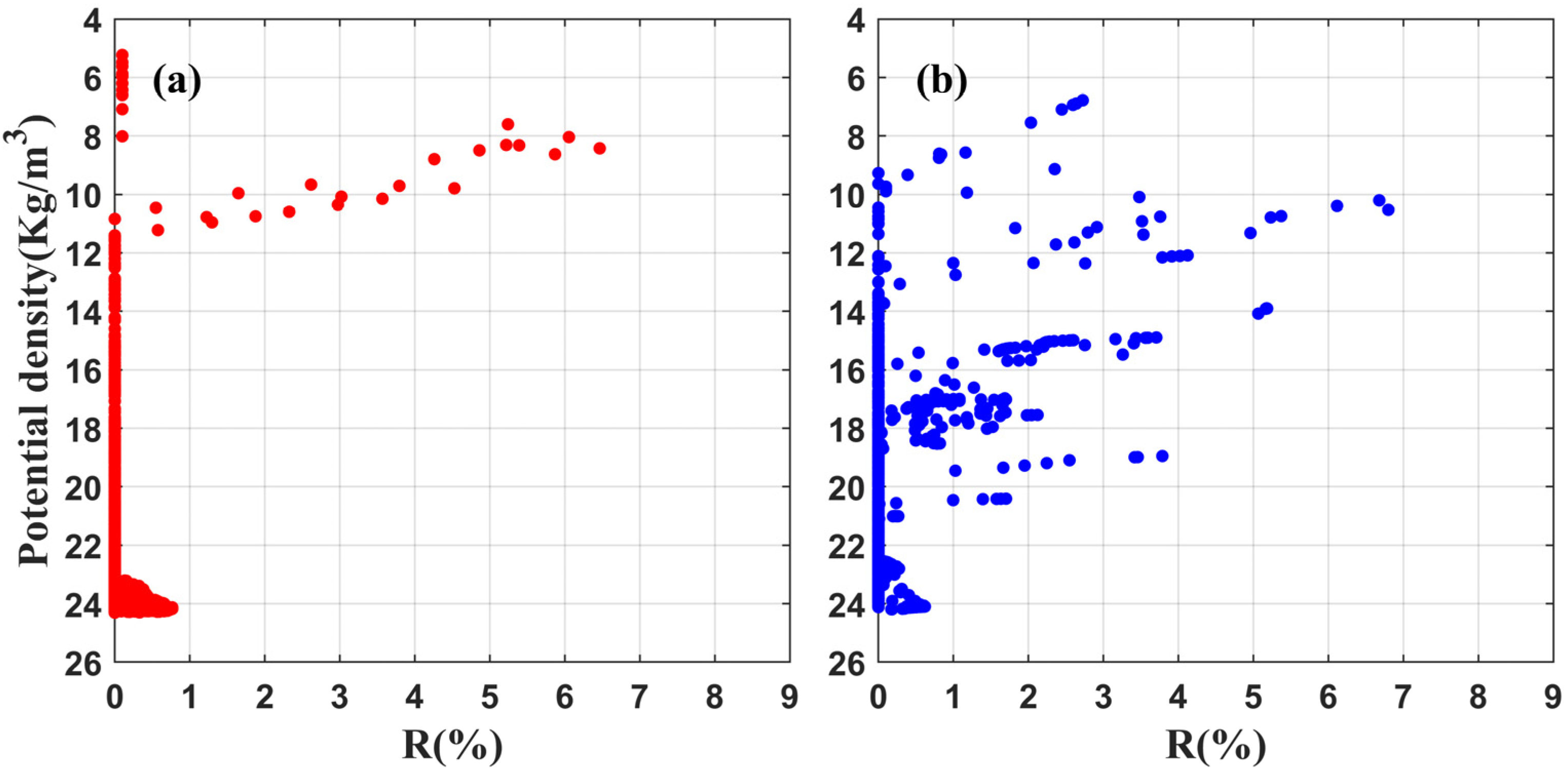
To solve the linear mixing equations, it is necessary to define a set of characteristic potential temperatures and salinities for each water mass as the SWTs. Figure 2 shows the T–S diagram for all observations. There are distinct ranges of potential temperature and salinity values. A most notable feature is that the potential temperature range is quite large, which is the reflection of intraseasonal variability. The T–S diagram clearly shows the existence of three types of water masses off western Guangdong: PR diluted water (PRDW) with the lowest salinity (<31 psu), SCS surface water (SCSSW) with high temperature and salinity, and SCS subsurface water (SCSSUW) with low temperature and high salinity. These characteristics are well-documented in previous studies [23,24,36]. Traditionally, the SWTs are defined by identifying prominent end members in T–S diagrams [37]. In this study, taking the intraseasonal variability of temperature and salinity into account, we define the core potential temperatures and salinities are (25 °C, 22 psu) for PRDW, (28 °C, 34 psu) for SCSSW, and (17 °C, 34.5 psu) for SCSSUW, respectively. The chosen values of each SWT are in good agreement with the results of Zhu et al. [23]. They suggested that the PRDW, SCSSW and SCSUW in spring are characterized by (26.55 °C, 29.17 psu), (28.24 °C and 33.80 psu) and (17.86 °C, 34.55 psu), which suggests that the properties of the samples in this study are well-represented by the set of SWTs considered.

3.2. Uncertainties

The mixing proportion of the SWTs is very sensitive to the chosen core potential temperatures and salinities. Mass balance residual (Rm) is often used as a measure of the uncertainty. Previous studies demonstrated that the range of 5–7% is the largest acceptable residual [28,31,35]. To assess the reliability of the OMP analysis, the mass balance residuals of all measurements from the two cruises are statistically analyzed. Figure 3 shows that all mass balance residuals are no more than 7%. The vast majority of the residuals (99% in April and 95% in May) are lower than 1%, which suggests that our results of the OMP analysis are believable based on the criterion of the mass balance residuals [34,35].

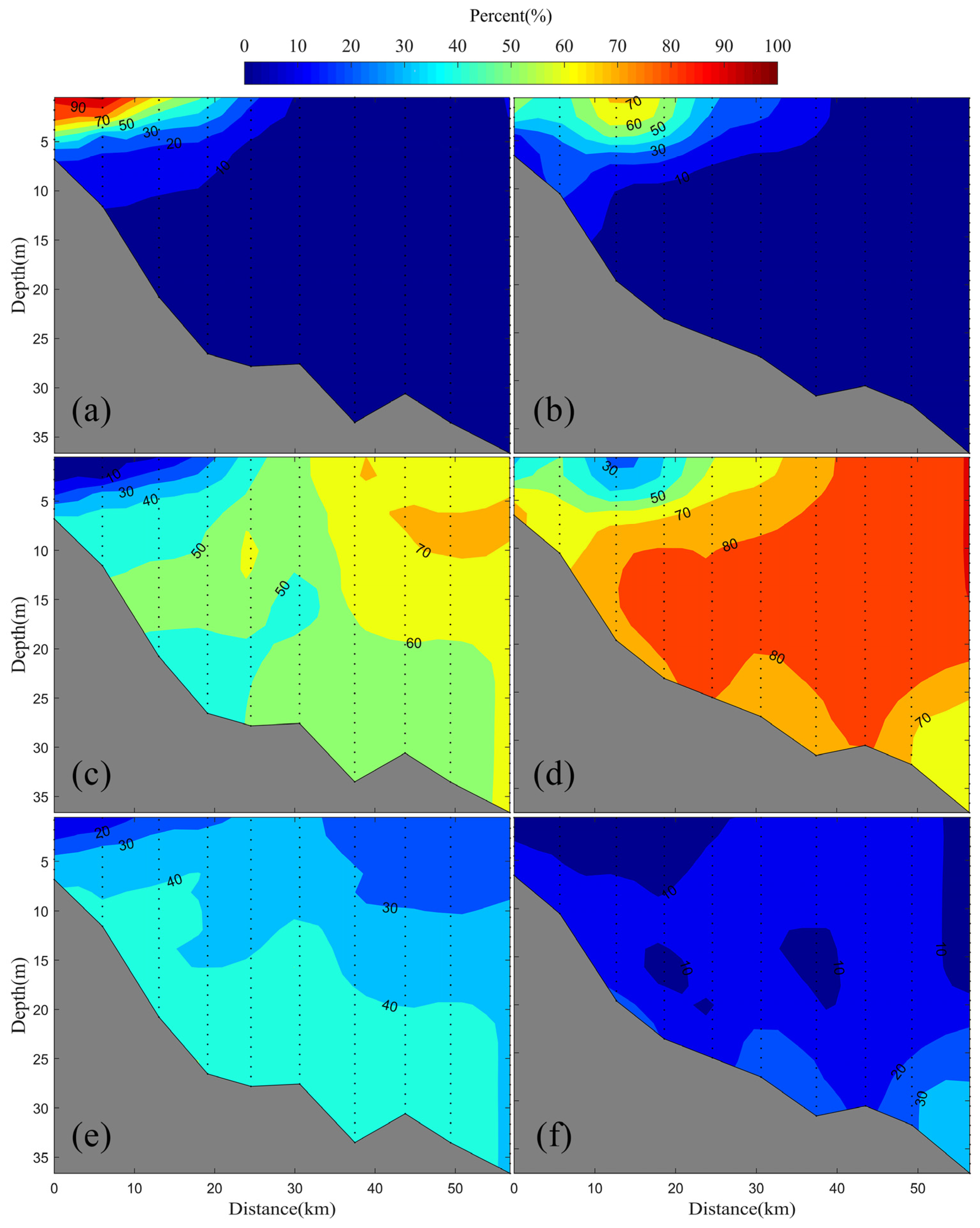
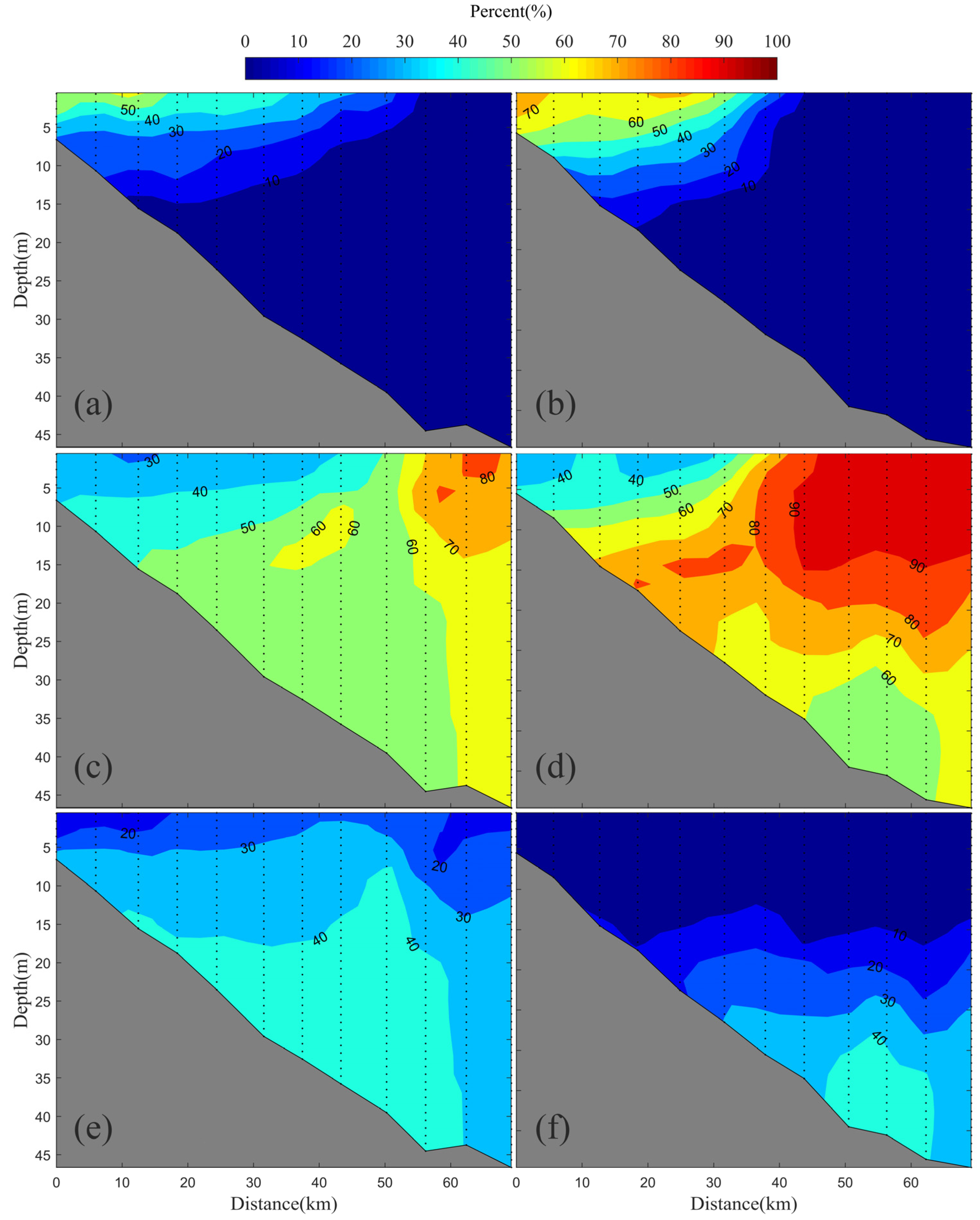
3.3. Water Mass Distributions

Figure 4 shows the proportions of each source at the surface for the April and May cruises. The surface water is essentially composed of PRDW and SCSSW, with a small contribution from SCSSUW. The three water mass sources present significant spatial and temporal variability. For the PRDW, it is primarily restricted to the nearshore waters with depths <30 m. During the April cruise, the highest contribution of the PRDW reaches as much as 100% near the coast, but sharply decreases to less than 40% near the 30 m isobath. In comparison, the PRDW spreads southwestward during the May cruise, with a weak decrease in the maximum contribution (~95%). A high contribution bulge appears between 112° and 113° E. For the SCSSW, this is mainly present in deep waters (depths > 30 m) with a contribution of >60% in April, and has a great increase (>90%) in May. For the SCSSUW, the intraseasonal variations are significant. The maximum contribution in April is less than 40% whereas its influence becomes negligible (<20%) in May.
Figure 5 shows the proportions of each source in the bottom layer for the April and May cruises. The dominant contributors are the SCSSW and SCSSUW. The PRDW is more confined to the nearshore region (isobaths < 10 m), forming a very narrow strip along the coast, with the contribution of ~40% for the April cruise. The strip gradually moves southwestward along the coast during the May cruise (Figure 5a,b). The SCSSW shows the largest contribution throughout the rest of the entire region for both the cruises. Its proportion is much larger in May (>70%), especially in the northeastern part east of 113° E, its maximum contribution reaches about 90%. For the SCSSUW, it shows a moderate contribution (~50%), the decrease in the proportion in May is apparent over the whole region. The relatively high core (~40%) present is centered at (112° E, 21° N). The changing trend in the proportion of the SCSSUW is generally in opposite to that observed for the SCSSW.
Figure 6 and Figure 7 show the contributions of the three SWTs in two typical sections where the intraseasonal variability of water masses is significant. The PRDW shows large contributions (>50%) within the upper layer (depths < 10 m). Along the T1 section, the PRDW has a high core centered at about 4 km (>90%) for the April cruise and at 15 km (~70%) for the May cruise, though its contribution slightly decreases. In contrast, along the T2 section, the PRDW contribution (>50%) shows a large increase and expands seaward about 35 km from the coast. For the SCSSW, it dominates in the remaining areas, with a maximum proportion of >80%. Its core identically spreads onshore and appears below the PRDW along both sections. The intrusion however is much stronger along the T1 section than along the T2 section. Near the bottom, the SCSSUW plays a secondary role, with its maximum proportion <50%. A decrease in the SCSSUW contribution is more prominent during the May cruise for the two sections. This decrease is closely linked to the increase in the proportion of SCSSW coming from the outer seawater.

3.4. Factors Influencing Water Mass Variability

The observations show the most remarkable variability in the PRDW. Previous measurements and numerical model experiments demonstrated that the shape and extension of the PR plume responds quickly to the change of surface wind direction and strength [13,14,15,38,39,40,41,42,43]. To see how the wind influences the PRDW extension through regulating local circulation, the temporally averaged mean surface winds and OMGOAFS model currents during the two cruises are included for comparison. During the April cruise, the winds blow to the northwest, with a maximum speed <5 m/s (Figure 8a). The corresponding currents at all depths consistently flow northeastward (Figure 9, left panel). The highest PRDW for this period is mainly located near the PRE. During the May cruise, the winds change to the southwest and become stronger (Figure 8b). The wind strength is however not uniform. Relatively strong winds (>6 m/s) occur in the northeastern part, and gradually decrease towards the southwest. The dowelling-favorable winds drive a surface onshore Ekman flow (Figure 9b) to squeeze the PRDW against the coast, causing the PRDW band to become generally narrow and its thickness to increase. In addition, a strong southwestward surface coastal jet appears near the coast (Figure 9b) and transports much more PRDW to the southwest, leading to a significant extension. The response of the coastally trapped freshwater plume to downwelling-favorable winds is also supported by previous observational and theoretical studies [15,44,45,46,47].
The SCSSW contribution from April to May cruises increases dramatically throughout the whole water column, whereas the SCSSUW contribution decreases significantly. These variations are also closely associated with the presence of strong northeasterly winds. The downwelling-favorable winds result in the deepening of the offshore surface mixed layer which entrains more ambient water [15,45,47]. In the same time, the wind-induced surface Ekman flow advects the offshore water landward, thereby increasing the SCSSW contribution. To compensate for this onshore advection, the SCSSUW is forced to downwell beneath the SCSSW and flow seaward, leading to the decrease in the SCSSUW contribution. A similar pattern associated with freshwater plume during downwelling-favorable winds is reported in previous numerical studies [15,45,47].

4. Conclusions

In this study, we investigated the structures and intraseasonal variability of water masses off western Guangdong during the spring monsoon transition using two spring hydrographic data sets from April and May 2016 cruises. Three types of water masses are identified: PRDW (S = 22 psu, θ = 25 °C), SCSSW (S = 34 psu, θ = 28 °C) and SCSSUW (S = 34.5 psu, θ = 17 °C), which are in good agreement with present knowledge of the water mass in the study region. To quantify the contribution of each source water mass, the optimum multiparameter method is performed. The results show that the PRDW is mainly restricted to the upper 10 m layer near the coast, with its maximum contribution >90%. The vast majority of the water mass in the outer region is primarily controlled by the SCSSW, with a >50% contribution. In the bottom layer below 20 m, the water masses mainly consist of SCSSW and SCSSUW with contributions of ~60% and ~40%, respectively.
Pronounced intraseasonal variability of each water mass is present in the observations. During the May cruise, the PRDW extends southwestward along the coast, with a notable bulge between 112° E and 113° E. The SCSSW spreads onshore and is found below the fresh PRDW. The SCSSUW generally retreats offshore. By combining with the corresponding surface winds and OMGOAFS model currents, the significant intraseasonal variability is largely due to wind changes in direction and strength. The strong northeasterly winds not only result in an increased SCSSW contribution through triggering onshore Ekman transport, but also a strong southwestward extension of the PRDW through enhancing the southwestward-flowing coastal current.
The present study only quantifies the water mass contributions of PRDW, SCSSW and SCSSUW for the spring period. The three types of water masses in this region dominate all the year around [23,24,36], however, the contribution of each water mass in other seasons maybe exhibit significantly distinct spatiotemporal variability due to multiscale variability of the monsoon, PR outflow and coastal currents. Much more data are still needed to better understand the water mass variability under different environmental conditions. On the other hand, recent studies have suggested that nutrients [48] and planktonic ciliates [36] in the region could be used as indicators of water masses. Future research may attempt to introduce biochemical parameters as water mass tracers into the OMP analysis to provide more supplementary information of each water mass.

Author Contributions

Conceptualization—Z.H.; writing—original draft, H.L.; writing—review and editing, Z.H. and J.Z.; analysis—H.L., H.Z., G.X. and X.C.; all authors reviewed the manuscript. All authors have read and agreed to the published version of the manuscript.

Funding

This research is supported by the Frontier Science Research Project of the Chinese Academy of Sciences (No. QYZDJ-SSW-DQC022), the Innovation Group Project of Southern Marine Science and Engineering Guangdong Laboratory (Zhuhai) (No. 311020004), the National Natural Science Foundation of China (No. 41706205;4217060042), and the Southern Marine Science and Engineering Guangdong Laboratory (Zhuhai) (No. SML2021SP308).

Institutional Review Board Statement

Not applicable.

Informed Consent Statement

Not applicable.

Data Availability Statement

The data presented in this study are available on request from the corresponding author.

Acknowledgments

The authors would like to thank the captain, crews, and marine technicians of the R/V Zhanjiang Kediao for helping collect in situ hydrographic data, and Matthias Tomczak for providing the OMP analysis program package (https://omp.geomar.de/, accessed on 12 May 2021), the Remote Sensing Systems for providing CCMP (Cross-Calibrated Multi-Platform) wind analysis products (https://www.remss.com/measurements/ccmp/, accessed on 31 May 2021), and, the Copernicus Climate Change Service for providing the daily mean surface currents of Operational Mercator global ocean analysis and forecast system (http://marine.copernicus.eu/, accessed on 30 May 2021). We also would like to thank anonymous reviewers for their constructive comments and suggestions in improving the manuscript.

Conflicts of Interest

The authors declare no conflict of interest.

References

  1. Helland-Hansen, B. Nogen Hydrografiske Metoder; Scand, Naturforsker Mote, Kristiana: Oslo, Norway, 1916. [Google Scholar]
  2. Montgomery, R.B. Water characteristics of Atlantic Ocean and of world ocean. Deep Sea Res. (1953) 1958, 5, 134–148. [Google Scholar] [CrossRef]
  3. Li, F.Q.; Su, Y.S.; Wang, F.Q.; Yu, Z.X. Discussion of some concepts of the water mass by the theory of fuzzy sets. Oceanol. Limnol. Sin. 1986, 17, 102–110, (In Chinese with English abstract). [Google Scholar]
  4. Tomczak, M. Some historical, theoretical and applied aspects of quantitative water mass analysis. J. Mar. Res. 1999, 57, 275–303. [Google Scholar] [CrossRef]
  5. Haine, T.W.N.; Hall, T.M. A generalized transport theory: Water-mass composition and age. J. Phys. Oceanogr. 2002, 32, 1932–1946. [Google Scholar] [CrossRef]
  6. Tomczak, M.; Godfrey, J.S. Regional Oceanography: An Introduction; Elsevier Science: Oxford, UK, 2003. [Google Scholar]
  7. Morrison, A.K.; Frolicher, T.L.; Sarmiento, J.L. Upwelling in the Southern Ocean. Phys. Today 2015, 68, 27–32. [Google Scholar] [CrossRef] [Green Version]
  8. Kolodziejczyk, N.; Llovel, W.; Portela, E. Interannual Variability of Upper Ocean Water Masses as Inferred from Argo Array. J. Geophys. Res. Ocean. 2019, 124, 6067–6085. [Google Scholar] [CrossRef]
  9. Shuai, Y.P.; Chen, Y.C.; Liu, Z.J.; Ge, Z.M.; Ma, M.Z.; Zhang, Y.F.; Li, Q. Distribution of Pearl diluted water and its ecological characteristics during spring monsoon transitional period in 2016. J. Trop. Oceanogr. 2021, 40, 63–71, (In Chinese with English abstract). [Google Scholar]
  10. Liu, Q.Y.; Jiang, X.; Xie, S.P.; Liu, W.T. A gap in the Indo-Pacific warm pool over the South China Sea in boreal winter: Seasonal development and interannual variability. J. Geophys. Res. Oceans 2004, 109, C07012. [Google Scholar] [CrossRef] [Green Version]
  11. Wyrtki, K. Physical Oceanography of the Southeast Asian Waters; University of California, Scripps Institution of Oceanography: La Jolla, CA, USA, 1961. [Google Scholar]
  12. Shang-Ping, X.; Qiang, X.; Dongxiao, W.; Liu, W.T. Summer upwelling in the South China Sea and its role in regional climate variations. J. Geophys. Res. Ocean. 2003, 108, 3261. [Google Scholar] [CrossRef]
  13. Wang, G.H.; Li, J.X.; Wang, C.Z.; Yan, Y.W. Interactions among the winter monsoon, ocean eddy and ocean thermal front in the South China Sea. J. Geophys. Res. Ocean. 2012, 117, C08002. [Google Scholar] [CrossRef]
  14. Lai, Z.; Ma, R.; Gao, G.; Chen, C.; Beardsley, R.C. Impact of multichannel river network on the plume dynamics in the Pearl River estuary. J. Geophys. Res. Ocean. 2015, 120, 5766–5789. [Google Scholar] [CrossRef] [Green Version]
  15. Lai, Z.; Ma, R.; Huang, M.; Chen, C.; Chen, Y.; Xie, C.; Beardsley, R.C. Downwelling wind, tides, and estuarine plume dynamics. J. Geophys. Res. Ocean. 2016, 121, 4245–4263. [Google Scholar] [CrossRef] [Green Version]
  16. Shu, Y.Q.; Wang, Q.; Zu, T.T. Progress on shelf and slope circulation in the northern South China Sea. Sci. China Earth Sci. 2018, 61, 560–571. [Google Scholar] [CrossRef]
  17. Li, F.Q.; Su, Y.S.; Fan, L.Q. Discrimination analysis of water masses in the north area of the South China Sea. Trans. Oceanol. Limnol. 1987, 3, 15–20, (In Chinese with English abstract). [Google Scholar] [CrossRef]
  18. Li, F.Q.; Su, Y.S.; Fan, L.Q. Application of fuzzy mathematics method in water mass analysis in the northern South China Sea. Haiyang Xuebao 1987, 669–680, (In Chinese with English abstract). [Google Scholar]
  19. Fan, L.Q.; Su, Y.S.; Li, F.Q. Analysis of water masses in the northern South China Sea. Haiyang Xuebao 1988, 2, 136–145, (In Chinese with English abstract). [Google Scholar]
  20. Li, W.; Li, L.; Liu, Q.Y. Water mass analysis in Luzon Strait and northern South China Sea. J. Oceanogr. Taiwan Strait 1998, 2, 207–213, (In Chinese with English abstract). [Google Scholar]
  21. Tian, T.; Wei, H. Analysis of Water Masses in the Northern South China Sea and Bashi Channel. Period. Ocean. Univ. Qingdao 2005, 1, 9–12, (In Chinese with English abstract). [Google Scholar]
  22. Cheng, G.S.; Sun, J.D.; Zu, T.T.; Chen, J.; Wang, D.X. Analysis of water masses in the northern South China Sea in summer 2011. J. Trop. Oceanogr. 2014, 33, 10–16, (In Chinese with English abstract). [Google Scholar]
  23. Zhu, J.; Zheng, Q.A.; Hu, J.Y.; Lin, H.Y.; Chen, D.W.; Chen, Z.Z.; Sun, Z.Y.; Li, L.Y.; Kong, H. Classification and 3-D distribution of upper layer water masses in the northern South China Sea. Acta Oceanol. Sin. 2019, 38, 126–135. [Google Scholar] [CrossRef]
  24. Gao, Y.; Huang, R.X.; Zhu, J.; Huang, Y.X.; Hu, J.Y. Using the Sigma-Pi Diagram to Analyze Water Masses in the Northern South China Sea in Spring. J. Geophys. Res. Ocean. 2020, 125, e2019JC015676. [Google Scholar] [CrossRef]
  25. Li, D.H.; Zhou, M.; Zhang, Z.R.; Zhong, Y.S.; Zhu, Y.W.; Yang, C.H.; Xu, M.Q.; Xu, D.F.; Hu, Z.Y. Intrusions of Kuroshio and Shelf Waters on Northern Slope of South China Sea in Summer 2015. J. Ocean Univ. China 2018, 17, 477–486. [Google Scholar] [CrossRef]
  26. Tomczak, M., Jr. A multi-parameter extension of temperature/salinity diagram techniques for the analysis of non-isopycnal mixing. Prog. Oceanogr. 1981, 10, 147–171. [Google Scholar] [CrossRef]
  27. Tomczak, M.; Large, D.G.B. Optimum multiparameter analysis of mixing in the thermocline of the Eastern Indian Ocean. J. Geophys. Res. 1989, 94, 16141–16149. [Google Scholar] [CrossRef]
  28. Budillon, G.; Pacciaroni, M.; Cozzi, S.; Rivaro, P.; Catalano, G.; Ianni, C.; Cantoni, C. An optimum multiparameter mixing analysis of the shelf waters in the Ross Sea. Antarct. Sci. 2003, 15, 105–118. [Google Scholar] [CrossRef] [Green Version]
  29. Leffanue, H.; Tomczak, M. Using OMP analysis to observe temporal variability in water mass distribution. J. Mar. Syst. 2004, 48, 3–14. [Google Scholar] [CrossRef]
  30. Pardo, P.C.; Perez, F.F.; Velo, A.; Gilcoto, M. Water masses distribution in the Southern Ocean: Improvement of an extended OMP (eOMP) analysis. Prog. Oceanogr. 2012, 103, 92–105. [Google Scholar] [CrossRef] [Green Version]
  31. Frants, M.; Gille, S.T.; Hewes, C.D.; Holm-Hansen, O.; Kahru, M.; Lombrozo, A.; Measures, C.I.; Mitchell, B.G.; Wang, H.L.; Zhou, M. Optimal multiparameter analysis of source water distributions in the Southern Drake Passage. Deep-Sea Res. Part II Top. Stud. Oceanogr. 2013, 90, 31–42. [Google Scholar] [CrossRef]
  32. Gasparin, F.; Maes, C.; Sudre, J.; Garcon, V.; Ganachaud, A. Water mass analysis of the Coral Sea through an Optimum Multiparameter method. J. Geophys. Res. Ocean. 2014, 119, 7229–7244. [Google Scholar] [CrossRef]
  33. McKenna, C.; Berx, B.; Austin, W.E.N. The decomposition of the Faroe-Shetland Channel water masses using Parametric Optimum Multi-Parameter analysis. Deep-Sea Res. Part I Oceanogr. Res. Pap. 2016, 107, 9–21. [Google Scholar] [CrossRef] [Green Version]
  34. Zhou, P.; Song, X.X.; Yuan, Y.Q.; Cao, X.H.; Wang, W.T.; Chi, L.B.; Yu, Z.M. Water Mass Analysis of the East China Sea and Interannual Variation of Kuroshio Subsurface Water Intrusion Through an Optimum Multiparameter Method. J. Geophys. Res. Ocean. 2018, 123, 3723–3738. [Google Scholar] [CrossRef]
  35. Karstensen, J.; Tomczak, M. Age determination of mixed water masses using CFC and oxygen data. J. Geophys. Res. Oceans 1998, 103, 18599–18609. [Google Scholar] [CrossRef] [Green Version]
  36. Gu, B.; Wang, Y.; Xu, J.; Jiao, N.; Xu, D. Water mass shapes the distribution patterns of planktonic ciliates (Alveolata, Ciliophora) in the subtropical Pearl River Estuary. Mar. Pollut. Bull. 2021, 167, 112341. [Google Scholar] [CrossRef] [PubMed]
  37. Bograd, S.J.; Schroeder, I.D.; Jacox, M.G. A water mass history of the Southern California current system. Geophys. Res. Lett. 2019, 46, 6690–6698. [Google Scholar] [CrossRef] [Green Version]
  38. Ou, S.Y.; Zhang, H.; Wang, D.X. Dynamics of the buoyant plume off the Pearl River Estuary in summer. Environ. Fluid. Mech. 2009, 9, 471–492. [Google Scholar] [CrossRef] [Green Version]
  39. Wong, L.A.; Chen, J.C.; Xue, H.; Dong, L.X.; Guan, W.B.; Su, J.L. A model study of the circulation in the Pearl River Estuary (PRE) and its adjacent coastal waters: 2. Sensitivity experiments. J. Geophys. Res. Ocean. 2003, 108. [Google Scholar] [CrossRef] [Green Version]
  40. Ji, X.M.; Sheng, J.Y.; Tang, L.Q.; Liu, D.B.; Yang, X.L. Process Study of Dry-Season Circulation in the Pearl River Estuary and Adjacent Coastal Waters using a Triple-Nested Coastal Circulation Model. Atmosphere-Ocean 2011, 49, 138–162. [Google Scholar] [CrossRef]
  41. Ji, X.M.; Sheng, J.Y.; Tang, L.Q.; Liu, D.B.; Yang, X.L. Process study of circulation in the Pearl River Estuary and adjacent coastal waters in the wet season using a triply-nested circulation model. Ocean Model. 2011, 38, 138–160. [Google Scholar] [CrossRef]
  42. Zu, T.T.; Wang, D.X.; Gan, J.P.; Guan, W.B. On the role of wind and tide in generating variability of Pearl River plume during summer in a coupled wide estuary and shelf system. J. Mar. Syst. 2014, 136, 65–79. [Google Scholar] [CrossRef]
  43. Luo, L.; Zhou, W.; Wang, D. Responses of the river plume to the external forcing in Pearl River Estuary. Aquat. Ecosyst. Health Manag. 2012, 15, 62–69. [Google Scholar] [CrossRef]
  44. Mazzini, P.L.; Barth, J.A.; Shearman, R.K.; Erofeev, A. Buoyancy-driven coastal currents off Oregon during fall and winter. J. Phys. Oceanogr. 2014, 44, 2854–2876. [Google Scholar] [CrossRef] [Green Version]
  45. Moffat, C.; Lentz, S. On the response of a buoyant plume to downwelling-favorable wind stress. J. Phys. Oceanogr. 2012, 42, 1083–1098. [Google Scholar] [CrossRef]
  46. Rennie, S.E.; Largier, J.L.; Lentz, S.J. Observations of a pulsed buoyancy current downstream of Chesapeake Bay. J. Geophys. Res. Ocean. 1999, 104, 18227–18240. [Google Scholar] [CrossRef] [Green Version]
  47. Choi, B.-J.; Wilkin, J.L. The Effect of Wind on the Dispersal of the Hudson River Plume. J. Phys. Oceanogr. 2007, 37, 1878–1897. [Google Scholar] [CrossRef]
  48. Li, Q.P.; Zhou, W.; Chen, Y.; Wu, Z. Phytoplankton response to a plume front in the northern South China Sea. Biogeosciences 2018, 15, 2551–2563. [Google Scholar] [CrossRef] [Green Version]
Figure 1. (a) Bathymetry of the study region (outlined with a black box) and its surrounding area. (b) Location of CTD sampling stations off the western Guangdong in spring 2016. Red dots and blue circles correspond to the April and May cruises, respectively. Gray contours are the isobaths.
Water 14 00375 g001
Figure 2. T–S diagram for the two cruise measurements. Red (blue) dots represent April (May) observations. The contours denote the isopycnals (kg/m3).
Water 14 00375 g002
Figure 3. Plots of the calculated mass balance residuals against the potential density for the April (a) and May cruises (b).
Water 14 00375 g003
Figure 4. Water mass contributions (%) of PRDW (a,b), SCSSW (c,d) and SCSSUW (e,f) at the surface for the April (a,c,e) and May (b,d,f) cruises.
Water 14 00375 g004
Figure 5. Water mass contributions (%) of PRDW (a,b), SCSSW (c,d) and SCSSUW (e,f) in the bottom layer for the April (a,c,e) and May (b,d,f) cruises.
Water 14 00375 g005
Figure 6. Vertical contributions (%) of PRDW (a,b), SCSSW (c,d) and SCSSUW (e,f) along the T1 section for the April (a,c,e) and May (b,d,f) cruises.
Water 14 00375 g006
Figure 7. Vertical contributions (%) of PRDW (a,b), SCSSW (c,d) and SCSSUW (e,f) along the T2 section for the April (a,c,e) and May (b,d,f) cruises.
Water 14 00375 g007
Figure 8. Surface winds overlaid with wind speed (color shading, unit: m/s), averaged over 12–18 April (a) and 13–20 May (b) 2016.
Water 14 00375 g008
Figure 9. The mean CMEMS model currents at 0 m (a,b), 21 m (c,d) and 40 m (e,f), averaged over 12–18 April (a,c,e) and 13–20 May (b,d,f) 2016. The subtitle in each subplot indicates the corresponding time and depth. The dashed lines denote the water depths (in meters).
Water 14 00375 g009
Publisher’s Note: MDPI stays neutral with regard to jurisdictional claims in published maps and institutional affiliations.

