1. Introduction
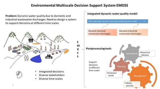
Water management is a complex task, seeking to balance human needs and ecosystem needs. In highly altered catchments with multiple stakeholders, water availability is often limited in terms of both quantity and quality. Stakeholders must make coherent and coordinated planning, management, and operational decisions. The scientific goal of this research is to design a system to respond to multiple needs at different time scales that can support the decision-making process of multiple stakeholders. To this end, the objective of this paper is to present two components of an environmental multiscale decision support system (EMDSS): an integrated dynamic model and three post-processing tools to test the usability of the model.
Decision support systems (DSSs) have been developed to integrate information and respond to specific objectives, allowing for decisions to be made on specific time- and spatial scales. One of the main obstacles to be dealt with in water management is the disconnection between the available information and the decisions to be made, and the integration of these decisions at different time scales, all of which lead to conflicts in water resources management [
1].
The most frequently used DSSs have been designed to support long-term planning decisions [
2,
3,
4]. These DSSs include platforms to compare planning strategies under uncertain conditions, such as climate change or population growth, and they focus on calculating water availability in terms of water quantity. When water quality is included, it is only verified at the end of the pipe. Water quality has become a limiting factor in highly altered catchments and should be analyzed to make decisions, not only about water uses, but also to guarantee river health and ecosystem function. For instance, Water Evaluation and Planning system (WEAP) [
5], Riverware [
6], or MODSIM [
3] can be coupled with QUAL2K [
7], given information about conventional water quality determinands.
Other DSSs for short-term decisions have been developed to operate reservoir systems and wastewater treatment plants, and to define Total Maximum Daily Loads (TMDLs) [
8,
9,
10]. Most of these include only some of the water quality determinands relevant to the systems’ operations, and not the complete set of determinands needed to make decisions for planning purposes [
9,
11,
12,
13].
The EMDSS designed and developed in this research to support the decision-making process in highly altered catchments includes an integrated water quantity and quality model for rivers, first developed by Luis Camacho [
14,
15,
16] in 1997. The Multilinear Discrete Lag Cascade—Aggregated Dead Zone—Quality Simulation Along River Systems model (MDLC-ADZ-QUASAR) [
14,
15,
16] was used to describe the dynamic behavior of a river, allowing the prediction of flow conditions using a hydrologic routing model (MDLC [
14]); a description of solute transport—i.e., advection-dispersion processes and the effect of dead zones in rivers [
17,
18] in the ADZ component; and water quality concentration through the integration of an extended QUASAR model to simulate reactive transport of conventional determinands [
15,
19,
20].
The integrated MDLC-ADZ-QUASAR model includes an unsteady flow routine that provides the option to support short-term operational decisions related to pollution events (minutes to days), medium-term management decisions (days to months), and long-term planning decisions (months to years). The water quality model implemented [
21,
22] includes almost the same transformation process as QUAL2K [
7] concerning the conventional determinands, such as organic matter, dissolved oxygen, nutrients, and pathogens. Others determinands, such as heavy metals, sulfides, manganese, and chlorides, are included in the MDLC-ADZ-QUASAR model as part of the present work to support decisions related to wastewater effluents from mining, agriculture, or industrial activities. In highly altered watersheds, a water quality model should include the inhibition of aerobic oxidation of organic matter and nitrification due to the lack of dissolved oxygen in the river. This condition is included in the proposed model and is not present in other models with similar characteristics [
23].
The dynamic water quality model was coupled with a model of urban [
24], industrial, mining, and agriculture wastewater discharges to evaluate variations in wastewater flows and their impacts in rivers.
The methodology to prove the usefulness of the integrated model at different timescales i.e., short-term (minutes to days), medium-term (days to months), and long-term (months to years), was the development of three postprocessing tools in the framework of the EMDSS, in a highly altered catchment with domestic and industrial releases. The study case includes the upper catchment of the Bogotá River in Colombia, one of the most polluted rivers in the world [
25].
First, to make long-term planning decisions, a definition of emission limits by industry type was conducted. Those limits should guarantee water quality goals (WQGs) defined to guarantee river health and ecosystem function [
26]. This approach would diminish externalities related to pollution in rivers, such as higher treatment costs and human health risks due to poor water quality. The tool uses a 24-year simulation period using the model in a steady state.
Second, a tool was developed to support medium-term management decisions (days to months) and to evaluate varying municipal withdrawal according to population growth. Water quality becomes a limiting factor in this scenario as various uses—human consumption, agriculture, livestock, and energy generation—are all considered. The tool can also be used to evaluate permitted limits on wastewater discharge concentrations per water quality determinand. In the tool, a two-year simulation period is run using monthly flow variations due to climate variability.
Finally, an operational decision short-term (minutes to hours) process was selected to assess the use of good water quality reservoir releases to maintain WQGs in the case of an upstream pollution event. A non-linear optimization algorithm was included to minimize the flow discharged by the reservoir, according to the water balance and self-purification process along the river. This process occurs in a time span of minutes to hours: the tool was developed using a two-day simulation period with an hourly timestep using the model in an unsteady state. For this contingent strategy, the reservoir releases used for hydropower generation downstream could have a double purpose, adding the improvement of water quality using dilution.
These three postprocessing tools were developed using the same dynamic integrated model and information organized in the EMDSS. This demonstrates that it is possible to develop a multipurpose EMDSS with different temporal scales, i.e., short-, medium-, and long-term, using the same platform.
2. Methods
This section presents a description of the integrated model and postprocessing tools. The proposed model is implemented in the upper Bogotá River basin—as explained at the end of the section—to demonstrate the usability of the model at the three temporal scales for planning, management, and operational decisions making.
2.1. Integrated Dynamic Model
To inform the analysis of water availability with water quality and quantity data, different models were defined and integrated into the EMDSS: a hydrological and surface water quality dynamic model for rivers including dead zones, developed by Luis Camacho [
14,
15,
16]; an empirical model to describe dynamic wastewater discharges by municipalities developed by Rodríguez [
24,
27] based on the model of Rodríguez et al. [
28]; and a new empirical model of dynamic wastewater discharges by industry. These integrated models enable users to make decisions at different time scales. Three algorithms are presented to support decision-making in terms of planning, i.e., months to years; managing, i.e., days to months; and operations, i.e., hours to days.
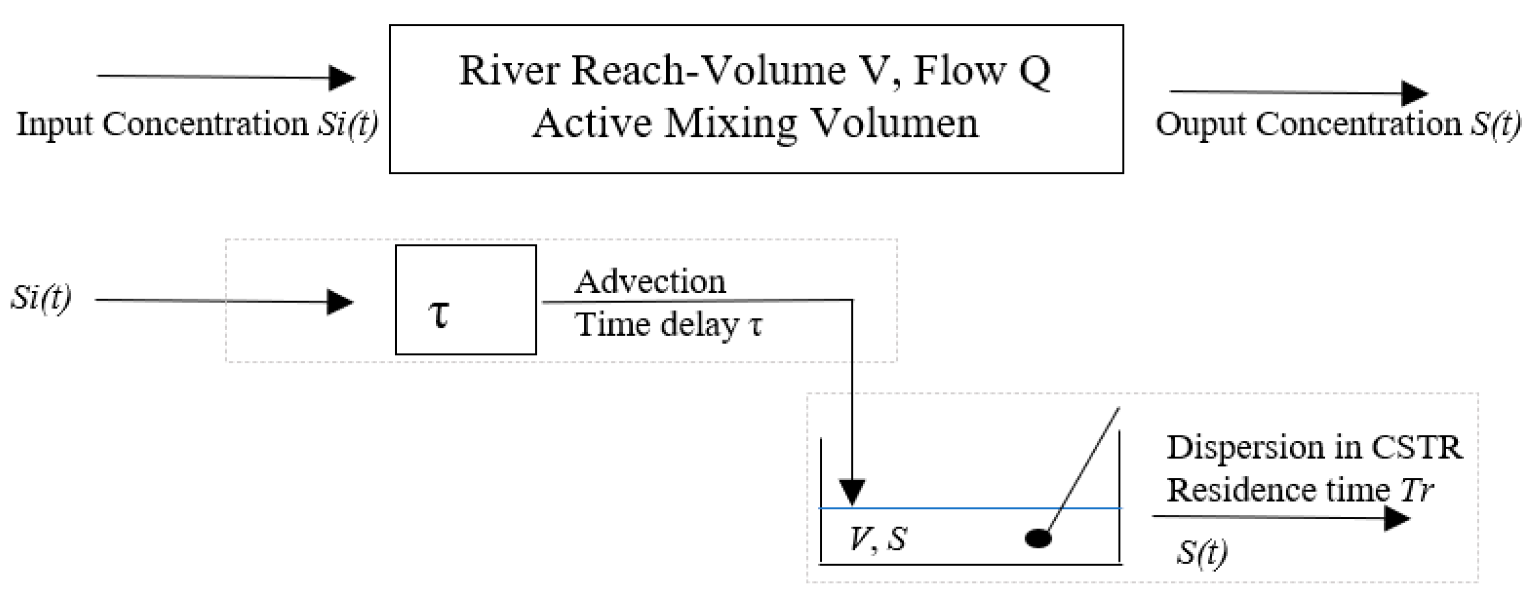
The conceptual structure of the integrated model is a lineal channel followed by a number of reservoirs in series, where solutes decay due to transport (
Figure 1) and reactions processes (
Figure 2). In the model, a river reach is considered as an imperfectly mixed system where a solute undergoes pure advection followed by dispersion in a lumped dead zone, i.e., dispersion in both the main channel and dead zones, as shown in
Figure 1.
Si(
t) is the known concentration at the input or upstream location,
τ is the advective time delay parameter introduced to describe solute advection due to bulk flow movement,
Q is the flow discharge and
V is the aggregated dead zone volume [
18].
2.1.1. Hydrologic and Surface Water Quality Dynamic Model for Rivers
The MDLC-ADZ-QUASAR model [
14,
15,
16] was used to describe the dynamic behavior of the river, allowing the prediction of flow conditions using a hydrologic routing model Multilinear Discrete Lag Cascade MDLC model [
14]. The Aggregated Dead Zone model ADZ was included to describe solute transport; i.e., advection-dispersion and the effect of dead zones in rivers [
17,
18], and the reactive transport of conventional determinands and toxic substances due to the integration and extension of the QUAlity Simulation Along River Systems (QUASAR) model [
15,
19,
20].
MDLC parameters are related to a linearized version of the Saint-Venant equation by the cumulant matching method. The results obtained with this model are as accurate as those obtained with the linearized Saint-Venant model. The number of reservoirs in the series are computed from hydraulic parameters, as in [
15]. The ADZ model [
17] is represented by an ordinary differential equation characterized by temporal parameters with clear physical significance. In this model, the dispersive effects are related to dead zone residence time and not to the diffusion term of the advection diffusion equation [
17,
20].
The MDLC and ADZ models have a similar structure, the same number of reservoirs in the series, and use an analog parameter relation to describe the flow and solute transport, allowing integration of the two models. The average propagation of the flow wave, i.e., the celerity, is higher than the solute transport mean velocity. This celerity and the solute velocity are related to the temporal parameters of the MDLC and ADZ models [
29].
QUASAR is a dynamic model for non-tidal rivers, describing the change over time of flow and water quality determinand concentrations. The model was coupled with the ADZ model to represent transport [
21], and water quality reactions are simulated during advection and dispersion times in the series of reservoirs.
The integrated model has the following capabilities desirable for the EMDSS:
The integrated dynamic model provides the option to incorporate dynamic and steady state discharges into the river. This is useful for highly altered catchments, where fluctuating wastewater flows generate dynamic water quality conditions in the river.
The integrated MDLC-ADZ-QUASAR model allows for the accurate simulation of advection, dispersion, and dead zone decay processes to describe solute and reactive transport.
The model can be used to support planning, management, and operational decisions by varying the timestep and simulation period. The dynamic behavior upstream of the river segment is characterized by yearly, monthly, or hourly factors and maximum, average, and minimum concentrations.
This model can forecast the travel time of pollution events to make operational decisions [
14].
The water quality determinands included in this model are those related to the domestic, industrial, mining, and agriculture discharges that may be found in highly altered catchments.
The general equation for the MDLC-ADZ-QUASAR model is obtained by incorporating the parameters of the MDLC-ADZ model into the general equation of the QUASAR model. A river reach is considered as an incompletely mixed system in which contaminant concentrations change due to pure advection—characterized by a temporal parameter of time delay
—and longitudinal dispersion modelled using the residence time of the solute in an aggregated dead-zone
. The extension of QUASAR to incorporate dead zones was made by Camacho; a detailed explanation can be found in [
15,
20].
Equation (1) presents a mass balance for
water quality determinand, where
is the upstream concentration,
is the downstream concentration,
is the residence time of the solute in the aggregated dead zone,
is the time delay and
k is the first-order reaction rate of the determinand [
15,
20]. The sources and sink terms of each determinand are described in the next section.
Sources and Sink Reactions for Water Quality Determinands
This model includes pollutants related to domestic, industrial, agriculture, and mining wastewater discharges. Conventional determinands, i.e., organic matter, nutrients, and bacteria, have been modelled, using the QUASAR model. The original model includes nitrate (
), dissolved oxygen (
DO), biochemical oxygen demand (
BOD), ammonium ion (
na), temperature (
T), pH, and conservative substances, e.g., chlorides (
Cl) [
20]. MDLC-ADZ-QUASAR includes oxidation reactions following their hierarchical order, i.e., aerobic respiration, denitrification, manganese reduction, sulfate reduction, chromium reduction, algae respiration, and methanogenesis. When the oxygen is depleted, those reactions are enhanced, giving rise to anaerobic conditions. The conventional pollutants are represented by incorporating fast and slow carbonaceous
BOD (
Cf and
Cs, respectively), detritus (
mo), total suspended solid (
TSS), inorganic suspended solids (
mi), ammonia (
na) organic nitrogen (
no), nitrates (
nn), organic and inorganic phosphorus (
po and
pi, respectively), conductivity (C), and pathogen indicators (
X) [
22].
Models of toxic substances are related to pH to describe the species of each determinand based on the chemical equilibrium principle. The pH model depends on alkalinity (
Alk) and inorganic carbon (
Ct). Some industries and mining activities discharge chromium (
Cr), sulfides (
Su), sulfates (
SO4), sulfites (
SO3), and chlorides (
Cl). Manganese (
Mn) is available in sediments (
MnO2) and soils and can be reduced under anaerobic conditions and released and resuspended to the river water [
30,
31]. The proposed model in this work was therefore extended to simulate pH and these toxic substances.
Figure 2 displays the conceptual water quality model including state variables and sources and sink processes. A mathematical model was developed for each state variable and detailed equations are shown in the
Supplementary Material (Equations (S1) to (S31)). Note that reduction and oxidation reactions between species of chromium, sulfur, and manganese not included in
Figure 2 are incorporated in the equations and in the model Petersen matrix (
Supplementary Material Table S2). According to the species for each water quality determinand, sedimentation, volatilization, or transport along the river is expected.
Each column in
Supplementary Material Table S2 is a water quality determinand and the sources and sink processes affecting each variable are represented by 1 and −1 respectively. For example,
Cs is diminishing its concentration (−1 in the Petersen matrix) due to hydrolysis and oxidation and is gaining concentration (1 in the Petersen matrix) due to dilution of detritus.
Cf is gaining concentration (1) due to dissolution of detritus and hydrolysis of
Cs; and
Cf is losing concentration (−1) due to
Cf oxidation and denitrification.
2.1.2. Integrated Municipal Wastewater Discharge Model
The dynamic behavior of river water quality is affected by multiple factors, including wastewater discharges and their temporal and spatial variations. Including time varying concentrations is often complicated by the lack of detailed information.
An integrated municipal wastewater discharge model previously developed by Rodríguez et al. [
24] was used as part of the EMDSS. The model includes the Urban Wastewater Generation Model (UWGM) [
28,
32], and an empirical model to predict state variables connected to the MDLC-ADZ-QUASAR model. The state variables modelled by MDLC-ADZ-QUASAR are:
T,
DO,
C,
Alk,
Ct,
pH,
BOD (both
Cs and
Cf),
na,
nn,
no,
po,
pi,
mi,
X,
mo,
Cr,
Sulf,
Cl,
Mn.
The Urban Wastewater Generation Model (UWGM) was used to estimate the mean flow,
BOD, and
TSS in municipal discharges, according to the number and type of users in the drainage system, i.e., household, institutions, commercial users [
28,
32], and their hourly variation for 24 h using deterministic and stochastic techniques [
32].
The empirical model based on linear (Equation (2)) and exponential (Equation (3)) multivariate correlations [
27] was used to estimate a time series for water quality determinands and flow for four municipal discharges in the upper Bogotá River catchment after wastewater treatment [
24]. The correlation between in-situ parameters and laboratory water quality analysis of each determinand was calculated. [
24]. The linear or exponential form of the correlation equation for each determinand was chosen according to the optimal correlation coefficient and the associated uncertainty was quantified [
24]. The 24-h normalized concentrations obtained in UWGM for
Q,
BOD, and
TSS in the discharge of each municipality were transformed by a set of scaling factors that match the minimum, average, and maximum normalized concentrations obtained with UWGM. After that, a denormalization of time series for the previous data and 24-h series was obtained. Those time series were calculated by Rodríguez and used in this research [
32].
2.1.3. Empirical Model of Dynamic Industrial Wastewater Discharges
Industry discharges alter river water quality dynamically. When the river has concurrent users, the dynamic behavior of the discharges overlap, generating water quality variations that are difficult to predict. Additionally, having detailed hourly information on each discharge is difficult, especially if these users do not have a treatment system that makes it possible to homogenize the discharge. However, information about daily variations of in-situ parameters in the river can be measured using automatic stations. This dynamic behavior can be used to describe the inflows and determine patterns along the river.
Industrial wastewater discharges vary not only according to the production process, but also by the chemicals and the wastewater treatment used. The degree of treatment should be defined to guarantee the water quality of the body receiving the effluent [
33,
34,
35,
36] as well as to achieve a maximum concentration for each determinand according to the industry [
33].
An empirical model was developed to characterize the wastewater effluents of the different industries and then to estimate the impacts of these discharges along the river. The models have two components: (1) definition of maximum, average, and minimum concentrations of flow and water quality parameters per industry type, and (2) determination of normalized hourly factors per water quality parameter to characterize the hourly variation of wastewater discharge.
The definition of maximum, average, and minimum concentrations of flow and water quality parameters was conducted using a dataset from the project “Dynamic modelling of Bogotá River” [
37], where information on thermoelectric and mining discharges was measured. This information was complemented with a literature review of maximum, average, and minimum concentrations for productive processes (tannery, brewery, and paper sector) before and after treatment (See
Table 1).
Daily variations of wastewater industrial releases were estimated from time-series measurements of river water quality, i.e.,
C,
pH, and
DO, using measurements from automatic stations along the river. Normalized minimum, average, and maximum values were determined for each hour of the day and for each in-situ determinand downstream of the inflow (
). The environmental agency (“Corporación Autónoma Regional de Cundinamarca”—the regional environmental authority CAR) [
38] supplied information of four automatic stations located along the upper Bogotá River. Monthly measurements taken every 5 min for 24 h were used to estimate hourly normalized concentrations for each in-situ water quality determinand.
Empirical mathematical models such as multivariate correlations for each determinand in the form of Equations (4) to (7) were obtained using the database compiled in the EMDSS. The optimal correlation coefficient between each in situ parameter i.e., C, pH, Q, and DO, and laboratory water quality parameter, i.e., BOD (Cs and Cf), na, nn, no, po, pi, mi, X, Cr, Sulf, Cl, mo, Mn, defines the empirical mathematical model to be used. In each water quality station, 20 to 30 samples were used in the statistical analysis. To obtain the best set of parameters for each determinand, Monte Carlo simulations were conducted to calibrate each regression. This group of time-series is ().
A 24-h scaling factor was obtained for each water quality determinand in each wastewater industrial discharge through the replacement of hourly normalized values of
C,
DO,
pH, and
flow (
) into each water quality determinand of the time series (
). Those normalized scaling factors were included in the MDLC-ADZ model.
Table 1.
Pre-treatment concentrations, National and Local emission limit concentrations in wastewater effluent by sector.
Table 1.
Pre-treatment concentrations, National and Local emission limit concentrations in wastewater effluent by sector.
| | | Domestic | Tanneries | Mining | Paper | Brewery | Thermoelectric |
|---|
| Det | Unit | Pre-
Treatment | National | Pre-
Treatment | National | Local | Pre-
Treatment | National | Pre-
Treatment | National | Pre-
Treatment | National | Pre-
Treatment | National |
| Temperature | °C | 21 | 40 | 13.5 | 40 | | 15.3 | 40 | 26.7 | 40 | 21.3 | 40 | 35.0 | 40 |
| Conductivity | μS·cm−1 | 2000 | | 3000 | | | | | 1373 | | 1000 | | 340 | |
| Oils and grease | mg·L−1 | 40 | 20 | 320 | 60 | 25 | 10 | 10 | 100 | 40 | 50 | 10 | 20 | 20 |
| TSS. | mg·L−1 | 275 | 90 | 1290 | 600 | 30 | 682 | 50 | 875 | 400 | 100 | 50 | 102 | 100 |
| Organic Nitrogen | mg·L−1 | 4 | | 200 | | 1 | | | 30 | | 10 | | 0.4 | |
| Ammonia | mg·L−1 | 4 | | 200 | | 1 | | | 30 | | 2 | | 0.7 | |
| Nitrates | mg·L−1 | 4 | | 200 | | 1 | | | 30 | | 2 | | 1.5 | |
| BOD | mg·L−1 | 400 | 90 | 2530 | 600 | 60 | 100 | 50 | 2000 | 400 | 175 | 100 | 300 | 150 |
| Organic Phos. | mg·L−1 | 5 | | | | 1 | | | 10.0 | | 8.8 | | 0.5 | |
| Inorganic Phos. | mg·L−1 | 5 | | | | 1 | | | 10.0 | | 8.8 | | 1.6 | |
| COD | mg·L−1 | 1000 | 180 | 4200 | 1200 | 120 | 200 | 150 | 5000 | 800 | 350 | 200 | 300 | 200 |
| Total Coliforms | UFC·
(100 mL)−1 | 1 × 10⁶ | | 1 × 10⁷ | | 5 × 10³ | | | 1 × 10⁶ | | 1 × 10⁵ | | 9 × 10⁵ | |
| pH | Und | 9.0 | 6–9 | 9.0 | 6–9 | 6–9 | | 6–9 | 9.0 | 6–9 | 9.0 | 6–9 | 7.1 | 6–9 |
| Total Chromium | mg·L−1 | 1 | 0.5 | 100 | 1.5 | 1 | 1 | 0.5 | | 0.5 | | | | 0.5 |
| Sulfate | mg·L−1 | 500 | | 2000 | | 400 | | 1200 | 2000 | 600 | | 250 | 0 | 250 |
| Sulfur | mg·L−1 | 0 | | 200 | 1 | 1 | | 1 | | 1 | | | | |
| Chlorides | mg·L−1 | | | | 3000 | 1100 | | 500 | | 1200 | | 250 | | 250 |
| Manganese | mg·L−1 | 0 | | 0 | | | 1 | | 0 | 0 | | | 0 | |
| References | | [39] | [33] | [40,41] | [33] | [34,36] | [42] | [33] | [43,44] | [33] | [45] | [33] | [46] | [33] |
2.1.4. Limitations of the Integrated Dynamic Model
The integrated dynamic model has limitations related to some determinands that are not yet included, such as pesticides, iron, lithium, oil and grease, and emerging pollutants. Diffuse loads are not yet included explicitly in the model, however domestic untreated wastewater and industrial point pollution sources provide, by far, the highest loads in the highly altered catchment of a developing country.
2.2. Three Postprocessing Tools Using the Integrated Dynamic Model
The selection of postprocessing tools to be used in this work was based on the needs of decision-makers, the type of stakeholder, and the timeframe of analysis. The tools are meant to support short-, medium-, and long-term planning, management, and operational decisions.
Three postprocessing tools were implemented in the framework of the EMDSS using the consolidated information in the database and the integrated model, MDLC-ADZ-QUASAR [
14,
15,
16], coupled with the dynamic and empirical model of wastewater discharges from municipalities [
24] and industries. The results are presented using visualization tools developed as part of the EMDSS.
Uncertainty analysis is performed for each model response in the developed tools. These analyses can be observed in the longitudinal profiles of the model that include associated confidence limits following the generalized likelihood uncertainty estimation (GLUE) methodology [
47].
2.2.1. Tool 1: Definition of Emission Limits by Industry
In this research, WQGs were defined to guarantee river ecosystem health [
26]. Consequently, various externalities can be avoided, including more expensive water treatment for human consumption, contaminated crops that could affect human health, soil degradation due to poor-quality irrigation water, and human health costs associated with pathogens in drinking water.
The integrated model was used to evaluate whether the goals would be fulfilled if the wastewater treatment mandated by regional and national laws were implemented by all users in the catchment. Scenarios with a projection of 24 years were developed assuming gradual changes to wastewater infrastructure and consequent effluent, and national and regional goals being reached in two to five years. A comparison between the concentrations and water quality goals was carried out and a conclusion was outlined about the viability of implementing this approach.
Emission limits by industry were evaluated using a multi-objective optimization algorithm adapted from a discrete dynamic programming model [
48] that seeks to maximize emissions of each industry, constrained by WQG compliance in the river (Equation (8)).
The emission concentration limits by industry (
ti) are discrete functions
Cind(
i) for each water quality determinand concentration
xi;
m is the number of determinands to be evaluated. Concentrations at the end of each river segment (
Ci+1) were evaluated using model simulations, where functions
Cind(
i) were assessed from upstream to downstream, following the model topology.
2.2.2. Tool 2: Extension of Intake Flows for Three Municipalities
Municipalities in the Bogotá River catchment are growing rapidly, and the river is the main water source for Bogotá, Suesca, and Tocancipá, Colombia. In this tool, an analysis was conducted to evaluate whether the river can fully meet water demand for all users (given projected population growth), while maintaining WQGs for ecosystem health and services.
A biannual projection of increasing demand was included in the integrated model, using population growth rates for each municipality. Hydrological scenarios of low and average flows were conducted, using emission limit concentrations. The analysis determined the available water, considering both quality and quantity.
2.2.3. Tool 3: Reservoir Operation to Improve Water Quality along the River
In some river basins, reservoirs are sources of water with good water quality that can be used to manage pollution events in rivers by dilution as a temporal or exceptional solution. To inform this operational decision, a tool following a multiobjective optimization algorithm was developed that uses the dynamic integrated water quality model to evaluate WQGs compliance at the end of each river segment downstream the reservoir releases.
The algorithm minimized the flow discharged into the river restricted by a discrete function of the reservoir operation curves
F[
qi,.,.
qn]. The algorithm finished when the concentrations downstream of each river segment
met WQGs, as shown in Equation (9). The concentrations downstream were evaluated using the integrated model included in the EMDSS.
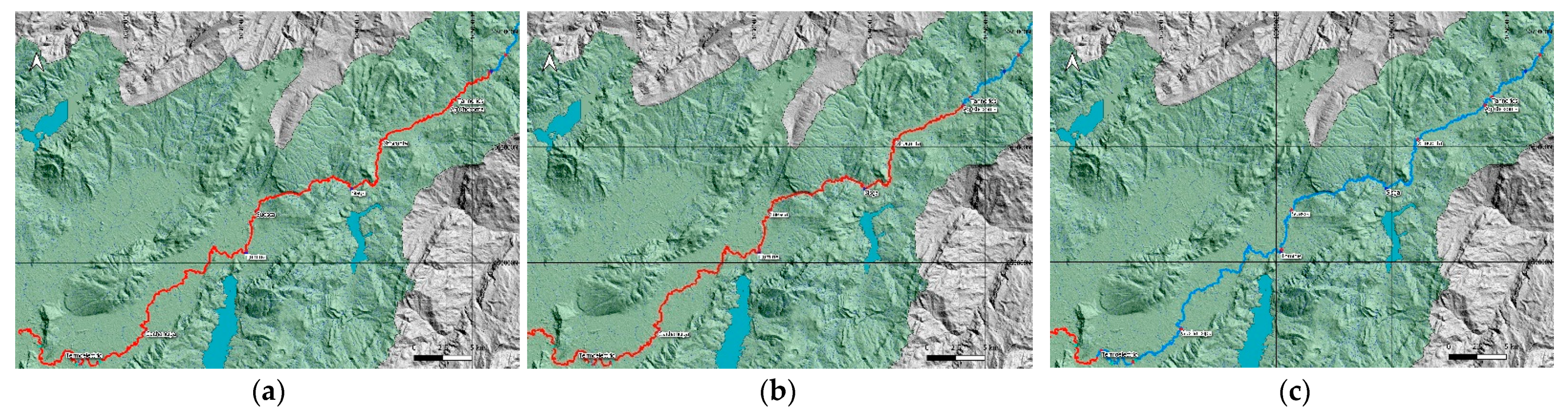
3. Case Study: Implementation of the Integrated Model along the Upper Bogotá River—Colombia
The first 99 km stretch of the Bogotá River, Colombia, was used for the implementation of the integrated model. The river headwater has an altitude of 2776 and downstream the altitude correspond to 2576 m.a.s.l. The width varies between 1.3 m and 9.2 m. The travel time is three to seven days, according to flow that has averages values in the upper gauging station (Villapinzón, Colombia) of 0.7 and in the lower gauging station (El Espino, Colombia) of 6.24 m3·s−1.This river stretch has six municipalities—Villapinzón, Chocontá, Sesquilé, Suesca, Gachancipá, and Tocancipá, Colombia—and 110 tanneries, two paper mills, a thermoelectric generator, a brewery, and agricultural users all discharging their treated and untreated wastewater effluents. Two reservoirs are located in this river segment: (1) Sisga at RK 38 (as measured from the headwater), with a volume of 94.3 hm3 and (2) Tominé at RK 52, with 690 hm3.
A total of 182 intakes along the river were reported by the regional environmental authority CAR for human consumption, agriculture, livestock, industry, and mining [
49].
Figure 3 depicts the Bogotá River, tributaries, discharges, intakes, gauges, and water quality stations. In the model, small tannery wastewater discharges are aggregated, as they are small intakes by type, e.g., agriculture. Tibitoc EAAB (“Empresa de Acueducto y Alcantarillado de Bogotá”, Bogotá’s water utility), at the end of the river segment, is a water supply facility for 30% or 2.4 million inhabitants of the city of Bogotá, Colombia.
The model was implemented and verified using an Excel platform executing a MATLAB code developed by Camacho (2016) [
21,
22] where the maximum, average, and minimum values and patterns from the mainstem, confluences, wastewater effluents, and intakes can be incorporated to represent their dynamic behavior. The spatial increment and time-step is about 0.05 to 0.2 h. The length of each river segment varies between 5 m to 300 m.
Model Information, Calibration, and Verification
The models used in this research have been implemented in the upper Bogotá River basin and calibrated using robust methodologies that allow for establishing the predictive capacity of the model and its associated uncertainty [
50].
The coupled model of the Bogotá River was calibrated in two phases: (1) the solute transport model MDLC-ADZ and (2) the reaction rates of all the water quality determinands of the model.
In the project “Dynamic Water Quality Modelling of the Bogotá River” [
37], all river confluences and main wastewater effluents along the 99 km of the upper Bogotá River were monitored. Solute transport processes were calibrated and validated using measurements of electric conductivity (8 h per day at 10-min sampling intervals) that were simultaneously obtained at different river stations. This monitoring was developed in 2009 [
25,
37]. The
n-Manning, Solute Lag Coefficient β and Dispersive Fraction DF parameters of the MDLC-ADZ solute transport model were calibrated [
29] using a tool developed in MATLAB, with the shuffle complex evolution (SCE-UA) methodology [
51] and analysis of the results using the generalized likelihood uncertainty estimation (GLUE) methodology [
47]. In this tool, the parameter, or parameters to be calibrated are selected and the Nash determination coefficient is used as the objective function. With this methodology, Nash coefficients of up to 0.95 are obtained in some reaches of the upper Bogotá River [
29].
In the same project, a comprehensive methodology to measure the dynamic behavior of rivers and inflows [
16,
25,
37] was conducted. Firstly, in situ parameters, i.e.,
Q,
T,
DO,
C, and
pH, were measured each 10 min in all sampling sites. Then, when conductivity presented a peak or valley and following MDLC-ADZ results, a sample was taken to analyze all of the parameters required to include in the dynamic water quality model. Conductivity has an important correlation with water quality determinand concentrations and was used as a surrogate variable [
27]. Three water quality campaigns under different hydrological conditions at 88 points, with 13 to 21 parameters per station were analyzed, and 54 reaches were used to characterize the dynamic water quality of the river. In addition, parameters, such as
Cr,
Sulf,
Mn,
Cl, were measured in other campaigns as part of MSc Theses and incorporated in this database [
31,
40,
52]. Calibrated rates were obtained in previous analyses [
31,
37,
40,
50,
52] using the SCE-UA [
51] and GLUE [
47] methodologies.
The UWGM was implemented and validated in Bogotá, Colombia, and other municipalities in the same river basin with similar consumption patterns and wastewater generation features. The calibration and validation process used data from 29 urban catchments. The normalized 24-h time series for
Q,
BOD, chemical oxygen demand
COD, and
TSS for four municipalities in the upper Bogotá catchment were generated in previous research. Detailed information of this time series generator developed by Rodríguez can be found in [
28,
32].
The wastewater treatment facilities of the municipalities in the study area are outdated and undersized, generating pollution problems along the river [
24]. Facultative ponds are implemented in these facilities, with treatment efficiencies of
BOD between 43% in Tocancipá, Colombia, and 95% in Suesca, Colombia, and
TSS between 17% in Chocontá, Colombia, and 90% in Suesca, Colombia [
53].
Measurements taken each 10 min for the three water quality campaigns of
Q,
T,
DO,
C and
pH were obtained from the wastewater discharges during a range from 3 to 10 h. Water quality samples taken in conductivity peaks or valleys were analyzed for other water quality parameters [
37]. Linear and exponential correlations were conducted to calculate the hourly time series for all determinands required for the dynamic model and the best performance was selected according to the optimal correlation coefficient [
24]. R
2 from 0.44 to 0.95 for water quality determinands were obtained with the optimal correlations, i.e., lineal or exponential (Equations (2) and (3)). Maximum, average, and minimum concentrations of each water quality parameter were obtained from the database compiled in this research from projects [
37,
54], and from biannual water quality campaigns conducted by CAR [
55] (
Table 2).
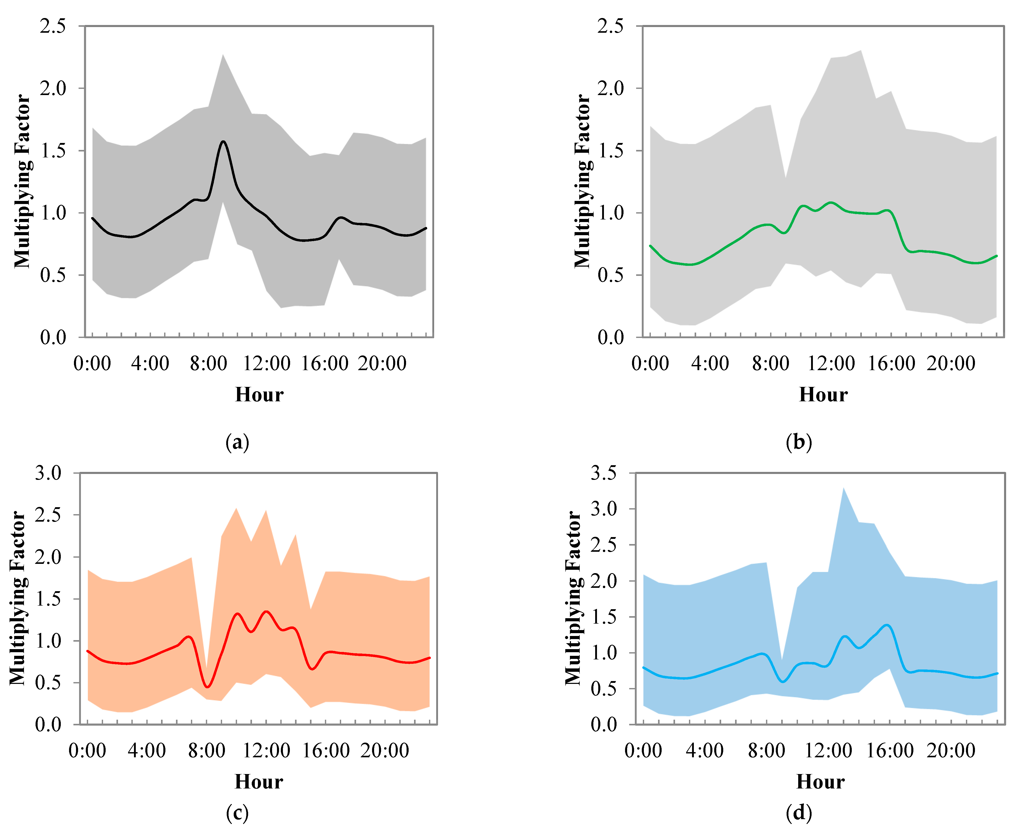
Figure 4 shows the normalized time series for
BOD for each municipality, as well as the hourly time-series for minimum, average, and maximum factors. These time-series show the dynamic behavior of each parameter per hour.
The industrial wastewater discharge model used information from four automatic stations located along the Bogotá River (see
Figure 3) [
38].
Figure 5 presents six days of those time series (
). Notice the inverse relation between
C (a) and
DO (b) and the short variation of
pH. This dynamic behavior of the river was used to describe the wastewater discharges, to characterize daily variation and represent the same signal along the river. This information is used to obtain hourly multiplying factors for wastewater discharges, obtaining mathematical models through multivariate correlations between the in situ parameters and water quality samples.
The EMDSS database includes information of each water quality station along the river for the upper Bogotá River [
31,
37,
40,
54,
56]. Water quality observations correspond to measurements taken by diverse stakeholders along the river: water quality data from 2002 to 2018 are obtained from the sub-national environmental agency in Cundinamarca CAR [
55]; and water quality modeling projects from 2002 [
54], 2009 [
37,
40], 2016 [
31,
40,
52] were integrated into the database. CAR took water quality samples twice a year, and currently analyzes 62 parameters, including conventional determinands, pathogens, heavy metals, phenols, and in situ characteristics, e.g., air and water temperatures.
The model was verified by simulating different hydrologic conditions (wet, average, and dry flow), and different load conditions (high, average, and minimum concentrations) for the tributaries and wastewater discharges; an example is shown in
Figure 6. The possible range of model responses is the area between the maximum and minimum simulations. Water quality observations (red dots) correspond to measurements along the river segment consolidated in the EMDSS. Verification consisted of confirming that the simulation minimum, average, and maximum values bracket historical data and follow the trends in each segment.
4. Description of the Postprocessing Tools and Results
Three postprocessing tools were developed to demonstrate the capability of the EMDSS and integrated model to support decisions at different time scales. The postprocessing tools used the information from the database and integrated model results to respond to specific needs for different stakeholders. In this section, the results of the implementation are presented.
4.1. Tool 1: Definition of Emission Limits per Type of Industry
An optimization algorithm was structured to obtain the maximum concentration for each determinand by industry in order to ensure WQGs. Discharges into the river were evaluated from upstream locations to downstream locations; as flow increases in this direction, the river gains assimilation capacity due to the dilution process. If the river is polluted upstream, more time and a longer distance are needed to achieve the desired water quality goal.
Discrete functions for each determinand emission concentration limit were defined as a range from national or regional limits up to possible values of post-treatment wastewater concentrations. Limits were defined per sector (tannery, brewery, paper, thermoelectric, domestic) to guarantee WQGs. In
Figure 7, the simulation results for fast
BOD Cf are presented as an example. The optimization algorithm fulfils the WQG progressing from upstream to downstream. The optimization process finishes when all segments meet the water quality goal or when the range of possible concentrations is surpassed.
Optimum loads to guarantee WQGs were obtained for the concentrations synthesized in
Table 3. For the thermoelectric facility, a lower concentration limit was defined because WQGs for
Cf and
DO were not fulfilled due to the high flow of this industry. According to the measurements of this discharge in the EMDSS database, it is possible to achieve the concentration limit proposed for the thermoelectric facility.
Figure 8 presents a
Cf concentration profile along the upper Bogotá River, expressing minimum, average, and maximum concentration values.
4.2. Tool 2: Expansion of Intake Flows for Three Municipalities
The Bogotá River is an important water source for the growing communities of Suesca, Tocancipá, and the capital city Bogotá, Colombia. This tool evaluates water availability for all users considering a flow increase for municipal water intakes, all while maintaining WQGs for ecosystem health.
A two-year projection of increasing demand was included in the integrated model, using the projected rates of population growth for each municipality. The hydrological scenarios defined were low and average flow, using regional limits for wastewater effluent concentrations proposed in the previous section, and tributaries accomplishing WQGs.
The analysis is presented using profiles of the river with load bands results for the hydrological scenarios, to provide the hydrological range for the decision-making process.
Figure 9 presents the daily flow measurements at Villapinzón, Colombia, from 1970 to 2018. Monthly climate variability was included in the model using the normalized average flow variation. Average (0.2 m
3·s
−1) and minimum flow (0.07 m
3·s
−1) at the headwater and increments in the Suesca, Tocancipá, and Bogotá, Colombia, intakes were simulated to determine whether the intake should be approved for meeting water quantity needs and ecosystem WQGs.
In
Figure 10,
DO (a) profile is presented, including inflows and outflows (b) along the river. At the end of the segment where Tibitoc is located, the oxygen level fell below 4 mg·L
−1. This means that if the intake expansions are approved, the
DO for the minimum and average flow at the end of this river segment will not fulfill the water quality standards. It is therefore not recommended to approve these permits because the water quality of the river will become polluted below WQG.
4.3. Tool 3: Reservoir Operation to Improve Water Quality along the River
In this river catchment, two reservoirs control water flow along the river and are used to guarantee enough water to hydropower generation downstream of this stretch. These reservoirs—Sisga (located in Chocontá, Colombia) and Tominé(Guatavita, Colombia)—could be used to guarantee the water quality downstream despite polluted discharges flowing into the river. For this example, untreated wastewater effluent from tanneries (10 to 16 river kilometers (RK)), paper factories (61 and 67 RK), a brewery (81 RK), and domestic discharges, i.e., Villapinzón, Colombia (8 RK), Chocontá, Colombia (27.9 RK), Suesca, Colombia (40 RK), Gachancipá, Colombia (72 RK) and Tocancipá, Colombia (79 RK) were considered.
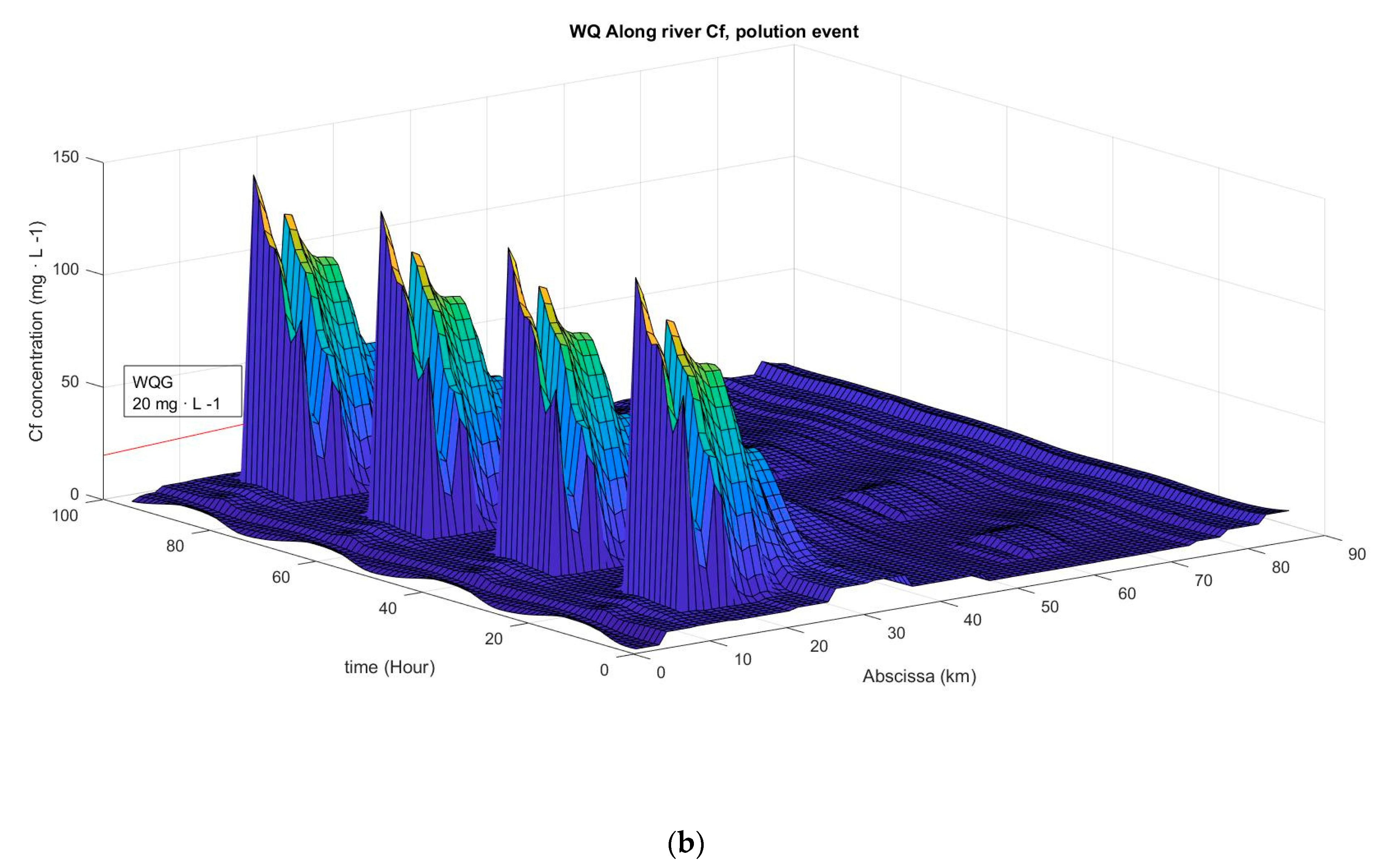
The minimum flow discharged by the reservoirs to fulfil the WQGs into the river was obtained with an optimization algorithm. The evaluation of WQG is performed at Suesca and Tibitoc intakes. For this evaluation, the integrated model simulates the polluted events from 8 am to 12 pm and the reservoir releases in an hourly timestep for 24 h. The dynamic behavior of the river and the response to pollution pulses can be visualized with the animation tool in QGIS and through 3D water quality profiles. 3D figures with the abscissa on the
x-axis, time (hourly) on the
z-axis, and determinand concentration on the
y-axis were developed and are presented in
Figure 11a,b.
A non-linear optimization algorithm was used to minimize the flow discharged into the river restricted by a discrete function of the reservoir operation curves. The algorithm finished when Cf, DO, TSS, ammonia, and the total coliform all met the WQGs that are defined as maintaining river health. According to flow measurements at each discharge, Sisga has an operation range of 0.012 to 6 m3·s−1 and Tominé of 0.1 to 10 m3·s−1.
In
Figure 11a, the first simulation of flows from Sisga—Chocontá, Colombia (0.012 m
3·s
−1) and Tominé—Guatavita, Colombia (0.1 m
3·s
−1) is illustrated. Notice how the polluted pulse is traveling downstream, diminishing the concentration of
Cf along the abscissa. For this example, reservoir discharges are not presented graphically. The WQGs were not fulfilled at either intake.
In
Figure 11b the effects of the reservoir discharges are illustrated graphically, with flows of 2.6 m
3·s
−1 and 6 m
3·s
−1 for Sisga and Tominé, respectively. The concentration of
Cf reached the goal of 20 mg·L
−1 in the two intakes defined as points for analysis: upstream of Suesca (40.6 RK) and upstream of Tominé (90.4 RK).
Table 4 presents simulation results of the optimization process to minimize flow in the two reservoirs to guarantee the WQG for
DO, Fast
BOD (
Cf), Total Coliform (
X), ammonia (
na), and Total Suspended Solids (
mo). When the Sisga and Tominé reservoirs discharged at 2.6 m
3·s
−1 and 6 m
3·s
−1, respectively, WQGs were fulfilled for
Cf,
na and
mo for Suesca and Tibitoc intakes. In Suesca, Colombia, the
DO reached a concentration of 4 mg·L
−1 (WQG) when the Sisga release was 6 m
3·s
−1 and in Tibitoc, Colombia when Tominé release was 6 m
3·s
−1. Neither Suesca nor Tibitoc intakes could reach the total coliform WQG.
Accordingly, the reservoirs could be part of a contingency plan to maintain water quality in the river, in the case of a pollution event upstream of the intakes. Two factors determine the viability of reservoir use: whether there is enough water stored to maintain flow, and whether water quality in the reservoir is good.
Table 4 presents the results of the optimization process for mean reservoir water quality concentrations measured together with reservoir discharges from 2002 to 2018. Average values in Sisga and Tominé of the total coliforms are above 30,000 and 19,000 UCF·(100 mL)
−1. Note that for total coliforms to be reduced to the maximum value safe for human consumption, a disinfection process must be implemented.
5. Discussion
Three postprocessing tools to support water resources decisions incorporating water quality were implemented successfully. In the long term, emission limits per sector were established to ensure WQGs fulfilment. In the mid-term, the expansions of city intakes were evaluated and in the short-term, the operation of two reservoirs to maintain water quality was examined.
Using the first tool, the evaluation of national and regional emission limits was conducted, concluding that, to guarantee water quality for health and ecosystem services, it is necessary to establish regional water quality emission limits for industry and municipalities that are more restrictive than the national emission limits. Currently, leather manufacturers have stricter emission limits along this river, and it is necessary to define more restrictive limits for municipalities and other industries. Limits for breweries, mining, thermoelectric, and paper industries, as well as domestic discharges were also defined for emissions to Bogotá River in order to guarantee water quality goals WQGs for human consumption with conventional treatment, agriculture and livestock.
The second tool implemented corresponds to the evaluation of flow expansion for three municipalities—Suesca, Tocancipá, and Bogotá, Colombia—taking water from the river. The analysis used population growth projections by the National Administrative Department of Statistics (DANE), Bogotá, Colombia, for two years. A statistical analysis of flow variability at the Villapinzón gauging station, Villapinzón, Colombia, allows for both wet and drought conditions to be considered. According to the simulations conducted on a monthly scale, the river has enough water to support the required flow increases but the water quality of the river could deteriorate below WQGs.
Finally, the third tool consists of the operation of two reservoirs to improve water quality in the river, if untreated discharges from tanneries, a thermoelectric facility, a brewery, and paper industries are occurring from 8 am to 12 pm. In this case, an optimization algorithm was developed to obtain the minimum flow required to guarantee WQGs defined to maintain river health for five parameters: DO, BOD fast Cf, TSS, ammonia, and total coliforms. According to the simulations carried out, with discharges of 2.6 m3·s−1 from Sisga and 6 m3·s−1 from Tominé, the river can recover the concentration to fulfil WQG of Cf, na and mo in both intakes Suesca and Tibitoc. DO could be recovered in Suesca if Sisga discharges 6 m3·s−1, and in Tibitoc, if Tominé discharges 6 m3·s−1. In any case, the total coliform cannot meet the WQG. The use of reservoir discharges to improve water quality in the river due to dilution relies on having sufficient volume and maintaining the reservoirs’ water quality. Otherwise, this contingency plan for pollution events cannot be used and the facilities should be closed.
6. Conclusions
In this article, a comprehensive description was provided of two important components of an EMDSS for highly altered catchments: an integrated dynamic model and three postprocessing tools to support operational, management, and planning decisions in the short-, medium- and long-term to shape a multitemporal scale analysis.
The integrated model MDLC-ADZ.QUASAR [
14,
15,
16] allows for analysis at different time scales by including an unsteady flow hydrological model, i.e., MDLC [
14]. This model is as accurate as the linearized Saint Venant equations for diffusion analogy flood waves. For catchments with a high dynamic flow behavior, this characteristic is particularly interesting because it can support decisions, such as the forecast of polluted events, as well as planning decisions. In this research, this conclusion is proved using the three postprocessing tools at different time scales.
The MDLC-ADZ-QUASAR model has been developed for conventional and toxic determinands, allowing analysis of domestic and industrial wastewater discharges. For domestic discharge, determinands, such as slow and fast BOD, inorganic suspended solids, DO, detritus, and pathogen indicators, are included, as well as nutrients, such as total nitrogen, ammonia, nitrates, and nitrites, and inorganic and organic phosphorous. Industrial discharges include some chemicals, such as chromium, sulfur, sulfates, sulfites, manganese, and chlorides. Therefore, pH, total inorganic carbon, and alkalinity are also included in this water quality model.
In this research, the integrated model was coupled with two empirical models to characterize the dynamic water quality behavior and maximum, average, and minimum concentrations of each determinand in the wastewater of industrial and municipal discharges. Both models are based on empirical relations between water quality parameters measured in situ and samples analyzed in the laboratory.
Three postprocessing tools were implemented to support short (hours to days), medium (days to months) and long (years to decades) term operational, management and planning decisions. The tools developed include:
Definition of emission limits per sector to guarantee river health and ecosystem services.
Increasing intake permits due to increasing demand.
Using reservoir releases to improve water quality along the river, in case of short-term pollution events
The results of the application to the case study of upper Bogotá River demonstrate that in a single EMDSS, short-, medium-, and long-term decisions can be integrated if the EMDSS incorporates a dynamic model and postprocessing tools. This feature provides decision-makers with comprehensive information in a single platform where decisions made at one scale can easily be transferred to other scales to meet the needs of different stakeholders, constituting a multi-scale and multi-objective EMDSS.
The Upper Bogota River has serious conflicts related to water quality, which require coordinated work among the stakeholders. Each of them manages the water resource at different spatial and temporal scales and their decisions are difficult to integrate. An EMDSS such as the one proposed allows decision makers to articulate efforts around integrated, appropriate, and readable information to improve their decisions.
According to this application in the Upper Bogotá River stretch, wastewater discharges of municipalities and industries should be more restrictive, to guarantee the water quality goals along river. Integrating these goals and management, the municipality intake expansions should consider, not only the among of water, but also the river water quality. Early warning alert systems could inform the volume of reservoir releases to maintain water quality goals in the river, in case of a pollution event.
In this research we design an Environmental Multiscale Decision Support System (EMDSS) that allows the decision-making process for diverse stakeholders and multiple objectives, using a dynamic model and postprocessing tools at different temporal scales. Different decision makers can use the same system integrating information and objectives to coordinated and articulate their decisions. The next step of this EMDSS is to make it available to decision makers to evaluate its acceptance and coordinated use among stakeholders.


