Article

Spatial Variability of the Mechanical Parameters of High-Water-Content Soil Based on a Dual-Bridge CPT Test

School of Earth and Environment, Anhui University of Science &Technology, Huainan 232001, China
*
Author to whom correspondence should be addressed.
Water 2022, 14(3), 343; https://doi.org/10.3390/w14030343
Submission received: 27 December 2021 / Revised: 20 January 2022 / Accepted: 21 January 2022 / Published: 24 January 2022

Abstract

:
Soft soil generally has a high water content, and the accurate quantification of its mechanical parameters is an important aspect of foundation design and disaster prevention. The mechanical parameters of soft soil have significant spatial variability or heterogeneity due to the complex deposition process of soil, leading to the high uncertainty of the quantifications of its parameters. Therefore, understanding the spatial variability of the parameters is an important approach to reduce uncertainty. In this study, the high-resolution (0.1 m) tip resistance (qc) and side friction (fs) of 18 soft soils in coastal areas were measured using the Dual-bridge CPT in-situ test. The vertical and horizontal variabilities of qc and fs were investigated using the random field theory. The results showed that both qc and fs are stationary and ergodic. The coefficient of variation of vertical fs is much higher than that of qc. On the one hand, fs may be vulnerable to noise, and its test accuracy is lower than qc; on the other hand, it may be that the spatial variability of the residual strength of soft soil may be greater than that of its failure strength. The horizontal correlation distance and coefficient of variation of qc and fs have no obvious change trend along the depth direction, but compared with the coefficient of variation curve, it was found that the change trends of qc and fs are basically the same, which is considered to be related to the properties of the soil layer. The research results can provide support for the spatial variability evaluation and reliability analysis of soft-soil engineering in this area. At the same time, it can also provide a theoretical basis for the layout of exploration engineering and sampling spacing.

1. Introduction

The soft-soil layer is widely and thickly distributed in China; it has the characteristics of a high water content, low density, low strength, high compressibility, low permeability and medium sensitivity. Among them, marine soft soil has poor engineering properties, such as a high rheological property, a low bearing capacity, poor permeability and the poor uniformity of soil layer [1,2,3,4,5,6]. In engineering construction, due to the nature of marine soft soil, engineering design and construction cannot achieve the desired results, resulting in a large number of diseases and security risks, causing engineering accidents. The further strengthening of the research on marine soft soil has important practical significance for the reduction and prevention of engineering accidents. In the study of the soft-soil layer, the accurate acquisition of the soft soil’s parameters is a very important prerequisite. As we all know, the physical and mechanical parameters of natural soil have significant spatial variability due to the different depositional environments and later geological function in the formation process, which is manifested in the discreteness and uncertainty of the parameter test values at different spatial locations. Through sampling tests or in-situ tests, only the parameters of soil at limited points in space can be obtained, and its parameter characteristics can’t be accurately measured point by point, which brings inconvenience to the reliability analysis of geotechnical engineering. Vanmarcke (1977) [7] first introduced the random field theory and established the random field model of soil profiling. Through the reduction of point variance, the transition from point characteristics to spatial average characteristics was completed, and the estimation of unknown point parameter characteristics through limited sample points was realized, laying the foundation for the study of the spatial variability of geotechnical parameters by random field theory. With the deepening of the research, the investigation of the spatial variation characteristics of soil parameters has been further developed and improved. At present, a complete system of data processing, stationarity and ergodicity tests, correlation distance calculation and site spatial variability evaluation has been formed [8,9,10,11,12,13], providing useful spatial variability parameters for geotechnical reliability design.
Soft soil is generally characterized by a high water content, low shear strength and high compressibility, such that it is difficult to obtain an undisturbed sample, which makes it difficult to study the spatial variability of their parameters through laboratory tests. Cone penetration tests (CPT) are a high-precision in-situ testing technique that enable continuous and rapid testing. They are an ideal method to study the parametric random field characteristics of soft soil. For example, Wang et al. (2009), Lin et al. (2015), Guo et al. (2017) and Qu (2021) [14,15,16,17] systematically investigated the random-field properties of soft soil along the coast of Guangdong, the sea-phase clay in central Jiangsu, and the coastal clay in Tianjin, China, using the cone resistance of the cone penetration test data, and statistically summarized the spatial variability of the soft soil parameters in the region. Many cone penetration tests on soft ground utilize a double bridge probe that measures the tip resistance qc and side friction fs. However, the above research results only carried out a random field analysis on cone penetration test qc, and lacked the study of random field characteristics based on side friction fs. The fs describes the shear strength characteristics of the soil after damage. The ratio of fs to qc is often used for the estimation of soft soil sensitivity, and fs is also often used to estimate the pile side friction. As such, the study of the random field model parameters of fs is also of practical importance. To this end, this paper takes the coastal soft soil in northern Jiangsu, China, as an example; based on the qc and fs data of the cone penetration test, this paper studies its spatial variability using the random field theory, and discusses the random field model parameters and their variation laws in the vertical and horizontal directions, respectively. The research results can provide parameter support for the reliability analysis of soft-soil engineering in this area.

2. Random Field Theory

2.1. Statistical Characteristics

In the Vanmarcke random field model, the soil profile is regarded as a random function of spatial position coordinates with autocorrelation characteristics, and the spatial variability of the parameters is regarded as a wave component varying around the mean value. When test errors are not considered, the measured soil profile test curve can be characterized by a trend function t ( h ) and a fluctuation function w ( h ) together [18], i.e., for a set of soil cone penetration test data x ( h ) , there exists:
x ( h ) = t ( h ) + w ( h )
In the formula, h denotes the sampling depth; the Vanmarcke random field model is based on the weak stationarity assumption, which considers the mean and variance of geotechnical parameters in space as constants independent of spatial coordinates, and its autocovariance function depends only on the distance between two observations [19]. However, in practice, as shown in Figure 1a, due to the influence of geological factors, x ( h ) tends to show a certain trend with increasing depth, and does not satisfy the basic assumption of being weakly stationary. After a detrending treatment of the geotechnical parameters, their residuals w ( h ) can be considered to satisfy the assumption of a zero mean in being weakly stationary [20,21], as shown in Figure 1b.

2.2. Stationarity and Ergodicity of the States

The knowledge of whether the soil profile conforms to stationarity and ergodicity is a prerequisite for analysis by the random field model. The Vanmarcke random field model simulates the soil profile using a homogeneous normal random field (Gaussian stationary homogeneous random process). Therefore, the data analyzed by the Vanmarcke random field model must conform to the condition of a stationary random field in a mathematical sense. Secondly, the soil mass is a collection of infinite points, and the experimental data are the measured values of individual points. If the analysis results of the experimental points in a borehole are used to reflect the properties of the surrounding soil mass, the data used should have the ergodic properties of various states. It can be seen that whether the spatial distribution of the soil properties is stationary and ergodic is the key to the application of random field method in geotechnical engineering. For soil bodies, the random field model of the soil profile is constructed by using the random field theory, which requires that the random field model must have stationarity and ergodicity [10].
As shown in Figure 2, in the one-dimensional random field   X ( h ) = { x 1 ( h ) , x 2 ( h ) , } , X n ( h ) represents the nth sample function of the random field, n = l, 2...N. For any depth h, the mean value μ X ( h ) of the sample function X ( h ) is
μ X ( h ) = lim N 1 N n 1 N x n ( h ) = E [ X ( h ) ]
where N is the number of CPT test holes, and E [ X ( h ) ] is the mean function of all of the sample functions of the random process X ( h ) at parameter h, which is called the ensemble average. In the range ( h , h + τ ) , there exists the autocorrelation function R X ( h , h + τ ) :
R X ( h , h + τ ) = lim N 1 N n = 1 N x n ( h ) x n ( h + τ ) = E [ X ( h ) X ( h + τ ) ]
If the mean value of the one-dimensional random field sample function is constant, the autocorrelation function is ( h , h + τ ) , and the random field is said to be stationary. Let x ( h ) be a mean-square continuous stationary random field, and its average depth < x ( h ) > will be
< x ( h )   > =   lim H 1 H 0 H x ( h ) d h
where, H is the sampling depth of the CPT test hole, if
< x ( h )   > =   μ X ( h ) = E [ x ( h ) ]
Then the mean value of random field x(h) is ergodicity.
< x ( h ) x ( h + τ )   > =   lim H 1 H 0 H x ( h ) x ( h + τ ) d h
If < x ( h ) x ( h + τ ) > exists, then
< x ( h ) x ( h + τ )   > =   R X ( h ) = E [ x ( h ) x ( h + τ ) ]
The autocorrelation function of the process is said to have ergodicity [22].

2.3. Correlation Distance

In a random field model, if there is
lim τ τ Γ 2 ( τ ) = 2 lim τ 0 τ ( 1 Δ x τ ) ρ ( Δ x ) d ( Δ x ) = δ u
where τ = i Δ x , i is the multiple of the sampling spacing, Δ x is the initial sampling spacing, an ρ ( Δ x ) is the correlation function. when τ is large enough, τ Γ 2 ( τ ) approaches to a fixed value δ u ; δ u is called the correlation distance, and its value represents the autocorrelation distance of the soil parameters. Within the range of the correlation distance, the parameters have correlation, and if the distance is greater than this distance, there is no correlation. At present, there are many methods to solve the correlation distance [23]: (I) the Space Average Method, SAM; (II) the Average zero-span method, VXP; (III) the Bartlett method of sample autocorrelation function, BLM; (IV) and Autocorrelation function fitting, AMF, etc. The Space Average Method (SAM) and Autocorrelation function fitting (AMF) are the most commonly used methods [20,24].
SAM works through the variance reduction function Γ 2 ( τ ) to solve the correlation distance δ u . According to the definition of correlation distance, the standard deviation of the whole sample is calculated σ , a new set of data samples is formed by the mean of adjacent i sample points, and the variance V a r ( i ) of the data is calculated. In this case, the variance reduction coefficient Γ 2 ( i ) is:
Γ 2 ( i ) = V a r ( i ) σ 2
Take different i values, repeat the above process, and make the graph of the function Γ ( i ) i , when i takes a certain value, Γ ( i ) , which tends to be stable. Find the Γ ( i ) stationary point n, and using δ u = n Δ x Γ 2 ( n ) find the correlation distance.
AMF uses the autocorrelation function model to fit the autocorrelation coefficient of the fluctuation component of the soil parameter samples and find the correlation distance. In actual calculations, the correlation function ρ ( τ ) corresponding to spatial distance τ is calculated according to Equation (10), and then the fitting method is used to calculate the correlation distance:
ρ ( τ ) = ρ ( i Δ x 0 ) = E [ x ( h ) x ( h + τ ) ] = 1 n i k = 1 n i X ( h k ) X ( h k + i ) .
Common sample autocorrelation function models include the exponential function (SNX), the linear exponential correlation function (LNX), the exponential cosine function (CSX), and the linear-exponential-cosine model (LNCS), as shown in Table 1 [5,19,25,26].
It is worth pointing out that in geotechnical investigation, the sampling spacing in the horizontal direction is usually large, and it is difficult to obtain a large volume of sample data, such that the horizontal random field model and parameters cannot be calculated by the strict autocorrelation function fitting method. Therefore, the method to determine the horizontal random field parameters of soil is different from that of the vertical random field parameters of soil. VXP uses the average length d ¯ of the intersection of the soil parameters function curve r ( h ) and its trend function curve t ( h ) to solve the horizontal fluctuation range δ h . It is commonly used to solve the correlation distance under limited boreholes. The calculation formula is:
d = i = 1 n d i / n
δ h = 2 π d 0.8 d
where d i is the segment length, as shown in Figure 3.

2.4. Coefficient of Variation

The coefficient of variation is one of the important indicators to characterize the internal variability of soil layers. Phoon and Kulhawy suggested the use of the inherent coefficient of variation C o v w instead of sample variance to characterize the internal variability of soil [9], and the calculation formula is
Cov w ( h ) = σ w ( h ) t ( h )
where t ( h ) is the trend item of the soil parameter test data, and σ w ( h ) is the standard deviation of the fluctuation component of the same soil parameter.

3. Application and Discussion

3.1. Project Profile

The Guanhe River embankment project in Guannan County, Lianyungang City, Jiangsu Province is the research object, as shown in the Figure 4; the site is located in the north of the Northern Jiangsu Plain, close to the Yellow Sea. The ground elevation is 2–3 m, the terrain is relatively flat, and the landform characteristics belong to marine plain accumulation landforms. The main structural feature in the site is the Cathaysian Huaiyin–Xiangshuikou fault, which extends into the Yellow Sea at an angle of 35–45°. No signs of activity have been found in the late and recent times, and the regional geological stability is good. The site is based on the epimetamorphic rock series in the mesoproterozoic area, the main cover layer is composed of the Sinian system to the Triassic system, and the upper quaternary system is mainly a marine-deposit soil layer. The silt layer of the marine deposit in the east of the site gradually thickens.
The boreholes and CPT holes for the geotechnical investigation and construction are mainly arranged along the Guanhe River embankment, with a total of 12 coring boreholes and 18 CPT holes. The physical and mechanical properties of the strata and each layer divided according to the site CPT test data and drill core data are shown in Table 2. As can be seen from the table, the soil layer of site 21 is mucky soil, which is close to the surface and mainly affected by marine accumulation. The thickness of the layer is great, with an average thickness of 16.3 m. It has the characteristics of high compressibility, low strength, high water content and high sensitivity; it is the main soil layer affecting the stability of the embankment. At the same time, the soft-soil layer is also the main object of this paper.
The CPT test adopts a standard double bridge probe, which can test the tip resistance qc and side friction fs. The probe penetrates into the soil by the static pressure method, the penetration rate is 1.2 m/min, the penetration reading interval is 0.1 m, the field zeroing error is less than 3%, the average spacing of CPT holes is 18.7 m, the hole layout position is shown in the Figure 5, and the test curve of typical CPT test holes and soil stratification results are shown in the Figure 6.

3.2. Outlier Test

For a group of soil sample test data, due to sampling methods, test methods and other reasons, abnormal data will inevitably appear, which affects the representativeness and authenticity of the data. Therefore, the test data must be checked for outliers. There are many methods in outlier testing: the 3σ test, Grubb’s test, the T-test, and the jump degree test, etc. [24,27,28,29]; the 3σ test is one of the most widely used methods. The basic steps are the determination of the mean μ and standard deviation σ of the sample, the construction of a valid data range (μ − 3σ, μ + 3σ), and the testing of the sample values one by one; outside the interval range is abnormal data, which should be discarded.
The tip resistance qc and side friction fs of CPT hole C514 in the site were taken as examples and tested by the 3σ test method. In order to visually illustrate the valid range of the data, we made 3σ graphs of qc and fs, as shown in Figure 7. As can be seen from the graph, the 3σ test shows that the tip resistance qc data of the C514 exploration hole were within the valid range, and there were no abnormal data, while the abnormal data of fs were deleted. The same method was used to test the abnormal values of other boreholes, which provided effective data support for subsequent random field analysis.

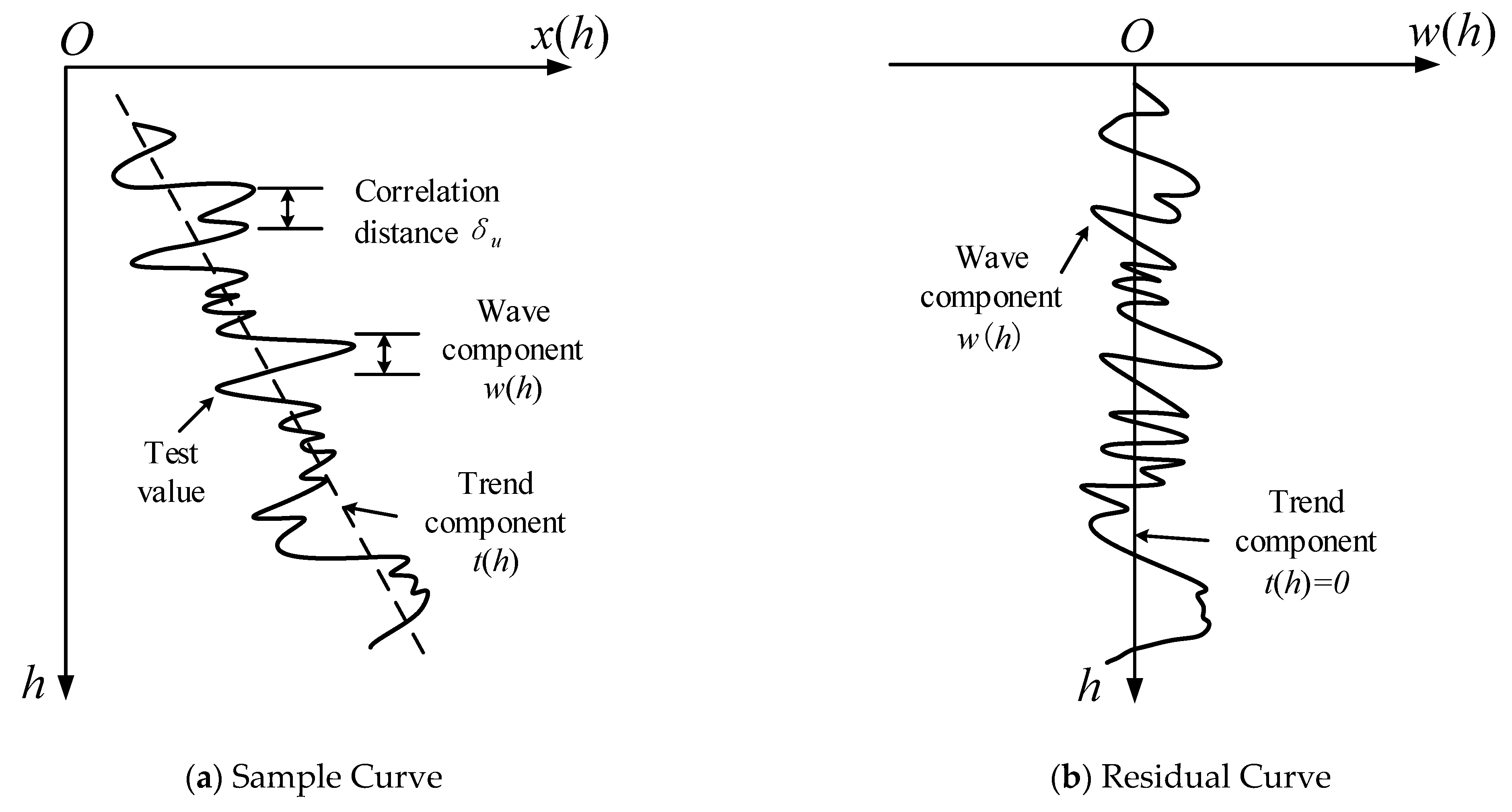
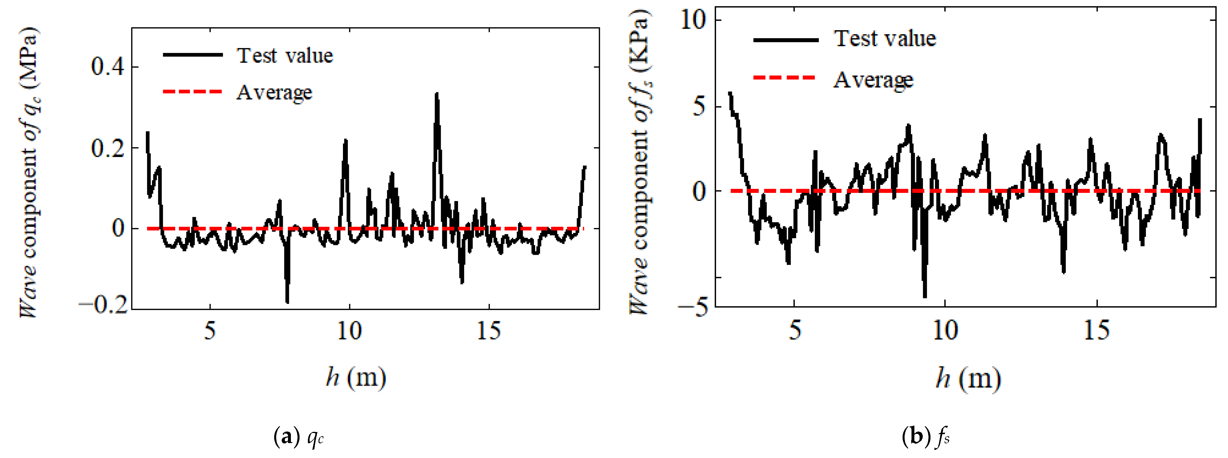
3.3. Trend Removal Processing

The tip resistance qc and side friction fs obtained by the CPT had a clear trend along the depth. In order to satisfy Vanmarcke’s assumption of the weak stability of a random field, it was necessary to detrend the original data [30]. Numerous studies have found that the trend component functions of the soil parameters are mostly linear, with a few higher-order functions, and suggested that the highest choice of trend function is no more than a quadratic nonlinear function [19,20]. Similarly, taking the C514 CPT test hole data as an example, linear and quadratic polynomials were used to fit the trend function, respectively, as shown in Figure 8. It can be seen that the fitting results of the two methods of qc are basically the same. In order to facilitate a calculation, the linear trend function was selected to determine that the trend term of the tip resistance was qc = 0.0383 h + 0.1888. For fs, it was found that the quadratic nonlinear function fits better than the linear function, and its trend item was fs = 0.100 h2 − 1.56 h + 16.94. We can then subtract the trend item from the original value to get the data curve of the detrended fluctuation item. Figure 9 shows the detrended result of this hole.
It can be seen from Figure 9 that the data of the tip resistance and side friction after trend removal fluctuated up and down on the axis of 0, only showing the volatility of the data, and the trend removal effect was good. The qc and fs data of other CPT holes underwent trend removal by the same method. Based on this, the fluctuation components (residuals) of qc and fs of all of the CPT test holes of marine mucky soft soil in the site could be obtained.

3.4. Stationarity and Ergodicity Tests

Based on the qc and fs data of 18 CPT holes of the marine soft-soil layer, i.e., soil layer 21, and the test principle of random field stationarity and ergodicity in the previous section, the relevant programs were compiled by Matlab 7.0 software. The results were as follows:
From Figure 10 and Figure 11, it can be seen that the ensemble average and correlation functions of the tip resistance qc and side friction fs of the marine mucky soft-soil layer at the site did not vary significantly along the depth direction, indicating that each sample of the soft soil random field did not change with the depth in the sense of probability, and the random field of soil prodile has the stability. qc, fs and the depth correlation function have no change along the horizontal direction, indicating that the mean values of each sample function and the depth correlation function of the tested random field do not change with the horizontal distance in a significance of the probability, that is, the random field of the two parameters of the soil profile have ergodicity of each state, which can meet the requirements of random field modeling.

3.5. Vertical Correlation Distance Solution

The stability and ergodicity of the random field of the soil profile show that the muddy soft-soil layer can be analyzed using the random field model. Based on the random field theory introduced above, the commonly used SAM and AMF were used, respectively. Taking the qc and fs data of the C514 CPT drills’ silty soft soil as examples, the calculation of the vertical correlation distance was introduced in detail. For the solution of the recursive space method, the sampling interval was set as iΔz. Δz is the initial sampling interval of 0.1 m, and I = 1–10. The calculation results are shown in Figure 12.
It can be seen from Figure 12 that when the sampling spacing is small, the vertical correlation distance calculated by different sampling spacing changes little; with the increase of the sampling spacing, due to the decrease of data points, the volatility of the calculation results based on qc and fs data increases, such that the variability of the soil parameters is homogenized, and the reliability of the correlation distance is greatly reduced, which cannot characterize the autocorrelation characteristics of real soil. According to the previous research results, when iΔzδu, the calculated correlation distance is more appropriate as the soil autocorrelation distance [31]. Thus, for qc, select 5Δz as the correlation distance corresponding to it is 0.55 m; for fs, select 7Δz, as the correlation distance corresponding to it is 0.8 m.
In order to verify the calculation results of the recursive space method, the four autocorrelation function models described in the previous section (Table 2) were used to fit the qc and fs correlation functions. The function fitting results are shown in Figure 13.
From Figure 13, it can be seen that the two parameter correlation functions of qc at 3 m and fs before 5 m fit well, and after the above values there is a greater volatility and a poorer fitting effect. Some scholars suggested taking the first half of the correlation function of the soil layer for fitting after research [15,22,28]. Therefore, in this paper, the soil layer in the depth directions of 0–2.2 m and 0–5 m were used to fit the four functions of qc and fs, respectively. The results show that the two parameters were SNX functions with the best fitting effect and LNCS function with the worst fitting effect. It was concluded that the SNX fitting correlation function expression of qc is y = e−3.352|τ|, and the vertical correlation distance δ = 2/3.352 = 0.597 m. The expression of the SNX fitting correlation function of fs is y = e−2.423|τ|, and the vertical correlation distance δ = 2/2.423 = 0.825 m. Compared with the SAM, the calculation results are larger, which is in agreement with the research results of [25]. This indicates that the method of calculating the vertical correlation distance by qc and fs in this paper is reliable, and can provide a theoretical basis for the further analysis of the fluctuation range of the soft-soil layer in the site.
In order to reasonably determine the vertical correlation distance of the marine mucky soft-soil layer, and to obtain the calculation results with statistical characteristics, the SAM and the correlation distance method were used to calculate the results, respectively, according to the qc and fs data of 18 CPT holes in the site. The results are shown in Table 3. It can be seen from Table 3 that under the condition of multiple samples, no matter qc or fs, the calculation result of the vertical correlation distance of the correlation function method is still larger than that of the SAM, but the standard deviation of the SAM is smaller than that of the correlation function method. The fluctuation range of the qc vertical correlation distance of marine mucky soft soil is 0.100–0.624 m, the average value is 0.324 m, and the coefficient of variation is 38.9%. The fluctuation range of the fs vertical correlation distance is 0.188–0.942 m, the average value is 0.386 m, and the coefficient of variation is 62.8%.
For the marine soft soil, in this case, the coefficient of variation of fs is much higher than that of qc. On the one hand, it may be that fs is vulnerable to noise and its test accuracy is lower than that of qc, such that it shows high variability [26,32]; on the other hand, it may be that the spatial variability of the residual strength of soft soil may be greater than that of the failure strength. Of course, this speculation needs further verification. In addition, the variation ranges of both the qc and fs vertical correlation distances are larger than the fluctuation ranges of the coastal marine clays in central Jiangsu proposed by [14], reflecting that the spatial variabilities of the marine soft clays in central and northern Jiangsu differ greatly, and the geographical characteristics of both are obvious. At the same time, the coefficient of variation is also much higher than that of the central marine clays, showing higher variability characteristics. Comparing the physical and mechanical properties and the depositional environment of the soft soil in both, the depositional environment of the soft soil in the central and northern coastal areas of Jiangsu is different. From the Lianyungang Area in the north to the Yancheng area in the middle, and then to the Nantong area in the south, the sedimentary facies are littoral facies, lagoon facies and neritic facies in turn. The buried depth of the soft soil decreases from shallow to deep, the porosity ratio and water content decrease in turn, and the density increases in turn, showing obvious different characteristics.
Based on the vertical correlation distance of the soil layer above, the sampling interval of the rock coring test can be guided; that is, the sampling interval should be equal to or slightly less than the vertical correlation distance of the corresponding rock formation.

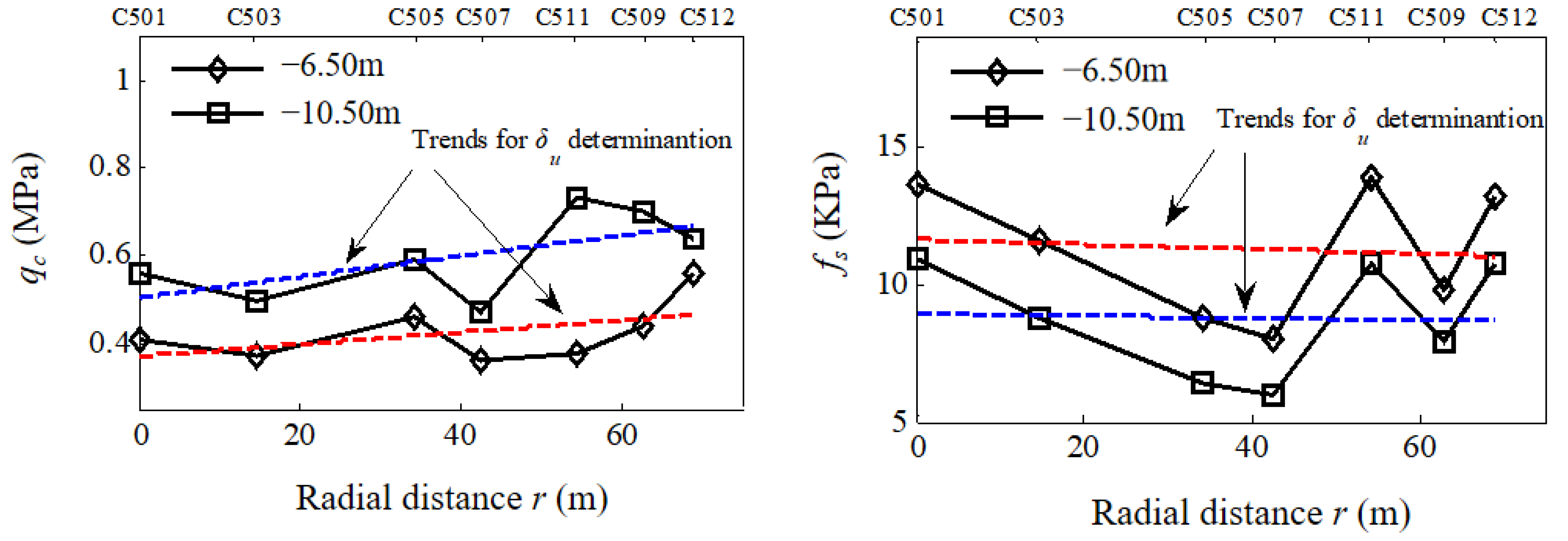
3.6. Horizontal Correlation Distance Solution

The horizontal correlation distance is also an important indicator to describe the spatial variability of soil. However, due to the fact that most CPT holes are not on a straight line and the spacing between the two holes is unequal, it is difficult to obtain enough and effective statistical samples, and the level random field model and parameters cannot be calculated by the strict autocorrelation function fitting method [33,34,35]. In view of this, VXP is used to calculate the horizontal correlation distance. VXP is suitable for the estimation of geotechnical parameters with a small parameter sample size, and its calculation results are similar to those of other methods. According to the previous work, it is considered that the test data of CPT holes with a radial distance of less than 20 m between the two holes are valid [35], and 7 of the 18 static exploration holes were selected as the exploration holes for the calculation of the horizontal correlation distance.
The data of qc and fs from seven boreholes at depths of −6.50 m and −10.5 m in the study soil layer were taken, respectively, and the correlation distances were calculated using the VXP, as shown in Figure 14.
As shown in Figure 14, in this case, the horizontal correlation distance of qc at the depth of −6.50 m was (63.0 − 9.6) × 0.8/3 = 14.2 m, and the fs horizontal correlation distance was (66.3 − 15.1) × 0.8/3 = 13.7 m. The horizontal correlation distance of qc at the depth of −10.50 m was (66.7 − 8.8) × 0.8/3 = 15.4 m, and the fs horizontal correlation distance was (63.8 − 14.2) × 0.8/3 = 13.2 m. The number of intersections between the sample curve and the trend function was greater than two, and the calculation results were reliable.
Lin et al. (2015) studied the variation trend of the horizontal correlation distance of Jiangsu marine clays with depth, and its relationship with the horizontal variation coefficient in the literature. It was concluded that the variation range of the horizontal coefficient of variation of Jiangsu marine clays was 5.0–11.1 m, with an average of 7.8 m, and the variation range of the horizontal coefficient of variation was 11.5–39.0%, with an average of 19.86%. The same method was used to analyze the horizontal spatial variability of the tip resistance qc and side friction fs of mucky soil 21 in this example. All of the test data of seven boreholes in the study soil layer were taken at an interval of 0.1 m. The calculation results are shown in Figure 15.
According to the calculation, the average horizontal correlation distance of mucky soil tip resistance is 19.18 m, the fluctuation range is 6.02–35.05 m, the coefficient of variation range is 5.8–163.5%, the average value is 53.8%, the average horizontal correlation distance of mucky soil side friction is 20.32 m, the fluctuation range is 7.23–32.27 m, the coefficient of variation range is 11.3–121.5%, and the average value is 52.6%; the horizontal correlation distance and coefficient of variation of the two parameters are basically the same, and have strong consistency. As can be seen from Figure 15, the variation range of the horizontal fluctuation range of qc and fs is large on the whole, both of which are greater than the reported values, showing strong variability and different regional characteristics. Moreover, the horizontal correlation distance and coefficient of variation of qc and fs have no obvious change trend along the depth direction. There is no significant correlation between the horizontal correlation distance of the two parameters and the coefficient of variation curve. However, by comparing the coefficient of variation curve, it was found that the variation trends of qc and fs are basically consistent, which is related to the soil properties. The coherence and variability of soil properties determine the consistency and variability of soil parameters. It should be noted that due to the limitation of the sampling spacing, the determination of the horizontal correlation distance of coastal soft soil in Northern Jiangsu is only based on relatively few exploration holes; the calculation result has a certain uncertainty, and can only be used as an approximate result. The results show that the parameters of the soil random field model are closely related to the observation scale, and this size effect should not be ignored in specific engineering applications. When the observation scale is too small, the statistical results have a great fluctuation, which is affected by the test error; when the observation scale is too large, the statistical results are affected by the geological environment, and the characterization of the soil spatial variability becomes weaker.

4. Conclusions

This paper systematically studied the evaluation method of the spatial variability of geotechnical parameters based on random field theory. Taking the marine mucky soil layer of the Guanhe embankment project in Guannan County, Lianyungang City, Jiangsu Province as an example, based on the test data from the CPT of a double bridge, the spatial variability was analyzed by random field theory, and the following conclusions were drawn:
  • Taking the marine mucky soil layer 21 of exploration hole C514 as an example, the 3σ rule was used to test the soil data for outliers, and the test results were good. Comparing the linear and non-linear fitting, the linear function was selected as the trend item for trend removal, and the processed data could be used to construct a random field model for the site soil layer.
  • The stationarity and ergodicity of the tip resistance qc and side friction fs data of mucky soil layer 21 were tested. The results show that the two parameters of the site soil layer had stationarity and ergodicity. Based on the SAM, the vertical correlation distances of tip resistance qc and side friction fs were 0.324 m and 0.386 m, respectively. The average coefficients of variation were 38.9% and 62.8% respectively. The horizontal correlation distances of tip resistance qc and side friction fs obtained by VXP were 19.18 m and 20.32 m, respectively, and the average coefficients of variation were 53.8% and 52.6%, respectively.
  • The variation coefficient of fs in the vertical direction is much higher than that of qc, and the correlation distance and variation coefficient in the horizontal direction are very consistent. Both of them show strong variability and different regional characteristics.
  • The borehole coring and borehole layout are very important for engineering investigation. The vertical and horizontal correlation distances have guiding significance for the borehole coring interval and borehole layout interval. In the project site, the sampling interval of the rock coring test will be equal to or slightly less than the vertical correlation distance of the corresponding rock stratum. The spacing of the holes will be equal to or slightly less than the horizontal distance of the corresponding rock stratum.

Author Contributions

Conceptualization, H.L. (Haifeng Lu) and X.M.; Funding acquisition, H.L. (Haifeng Lu); Investigation, H.L. (Haifeng Lu) and X.M.; Methodology, H.L. (Haifeng Lu); Validation, X.M.; Visualization, X.M. and H.L. (Huiying Li); Writing—original draft, H.L. (Haifeng Lu) and X.M.; Writing—review and editing, X.M. and H.L. (Huiying Li). All authors have read and agreed to the published version of the manuscript.

Funding

This study was partially supported by research grants from the major projects of natural science research in the Higher Education Institutions of Anhui Province (KJ2019ZD11), the Open Fund of State Key Laboratory of Coal Resources and Safe Mining (No. SKLCRSM20KFA06), and the National Natural Science Foundation of China (41977253). The data used in this paper can be accessed by contacting the corresponding author directly.

Institutional Review Board Statement

Not applicable.

Informed Consent Statement

Not applicable.

Data Availability Statement

The data used in this paper can be accessed by contacting the corresponding author directly.

Conflicts of Interest

The authors declare no conflict of interest.

References

  1. Duan, W.; Liu, S.; Cai, G. Evaluation of Engineering Characteristics of Lian-Yan Railway Soft Soil Based on CPTU Data-A Case Study. Procedia Eng. 2017, 189, 33–39. [Google Scholar] [CrossRef]
  2. Zhao, C.; Zhao, D. Application of construction waste in the reinforcement of soft soil foundation in coastal cities. Environ. Technol. Innov. 2020, 21, 101195. [Google Scholar] [CrossRef]
  3. Gao, Y.; Zhang, S.; Ge, X. Statistics of compression index of soft clay in coastal areas of China and comparison with other foreign areas. Rock Soil Mech. 2017, 9, 2713–2720. [Google Scholar]
  4. Jian, W.; Wu, Z.; Liu, H. Correlation analysis of CPT Parameters of soft soil in Southeast Fujian coastal area. Rock Mech. Rock Eng. 2005, 5, 733–768. [Google Scholar]
  5. Lin, J.; Liu, S.Y.; Cheng, Y.H.; Cai, G.J.; Fan, Q.J.; Li, C. Research and application of soft soil classification in Jiangsu Area based on pore pressure static penetration test. Chin. J. Geotech. Eng. 2021, 43, 241–244. [Google Scholar]
  6. Wang, Q.L. Working principle of static penetration and its application in engineering survey of Shanghai soft soil area. Urban Roads Bridges Flood Control 2021, 2, 221–223. [Google Scholar] [CrossRef]
  7. Vanmarcke, E.H. Probabilistic Modeling of Soil Profiles. J. Geotech. Eng. Div. 1997, 103, 1227–1246. [Google Scholar] [CrossRef]
  8. Onyejekwe, S.; Xin, K.; Louis, G.E. Evaluation of the scale of fluctuation of geotechnical parameters by autocorrelation function and semivariogram function. Eng. Geol. 2016, 214, 43–49. [Google Scholar] [CrossRef]
  9. Phoon, K.K.; Kulhawy, F.H. Characterization of geotechnical variability. Can. Geotech. J. 1999, 36, 612–624. [Google Scholar] [CrossRef]
  10. Yan, S.; Deng, W. Verification of stationarity and ergodicity of random field model of soil profile. Chin. J. Geotech. Eng. 1995, 17, 1–9. [Google Scholar]
  11. Jaksa, M.B. Inaccuracies Associated with Estimating Random Measurement Errors. J. Geotech. Geoenviron. Eng. 1997, 123, 393–401. [Google Scholar] [CrossRef]
  12. Dasaka, S.M.; Zhang, L.M. Spatial variability of in situ weathered soil. Geotechnique 2012, 62, 375–384. [Google Scholar] [CrossRef] [Green Version]
  13. Wang, G.; Jiang, W.; Qin, S.J.; Nie, L.Q. Application of dual-bridge static penetration test in soil division. Geotech. Eng. Tech. 2020, 34, 365–371. [Google Scholar]
  14. Lin, J.; Cai, G.; Zou, H. Evaluation of spatial variability of Jiangsu marine clay based on random field theory. Chin. J. Geotech. Eng. 2015, 37, 1278–1287. [Google Scholar]
  15. Wang, Y.; Wang, B.; An, Y. Study on random field characteristics of soil parameters based on CPT data. Rock Soil Mech. 2009, 30, 2753–2758. [Google Scholar]
  16. Guo, L.P.; Kong, L.W.; Xu, C. Determination method of autocorrelation distance of static penetration parameters and analysis of influencing factors. Rock Soil Mech. 2017, 38, 271–276. [Google Scholar]
  17. Qu, K. Application of static penetration in geotechnical engineering investigation of guangzhou-Foshan-Jiangmen-Zhuhai intercity rail transit line. Constr. Des. Proj. 2021, 8, 24. [Google Scholar]
  18. Stuedlein, A.W. Random Field Model Parameters for Columbia River Silt. Geotech. Spec. Publ. 2011, 224, 169–177. [Google Scholar]
  19. Baecher, G.B.; Christian, J.T. Reliability and Statistics in Geotechnical Engineering; John Wiley & Sons: Hoboken, NJ, USA, 2005. [Google Scholar]
  20. Cafaro, F.; Cherubini, C. Large Sample Spacing in Evaluation of Vertical Strength Variability of Clayey Soil. J. Geotech. Geoenviron. Eng. 2002, 128, 558–568. [Google Scholar] [CrossRef]
  21. Wang, J. Study on Spatial Variability of Mechanical Parameters of Ningbo Soft Soil. Master’s Thesis, Hubei University of Technology, Wuhan, China, 2019. [Google Scholar]
  22. Cheng, Q.; Luo, S.; Gao, X. Analysis and Discussion on calculating correlation distance by correlation function method. Rock Soil Mech. 2000, 3, 281–283. [Google Scholar]
  23. Yao, J. Research and Application of Spatial Correlation and Random Field Simulation of Geotechnical Parameters. Master’s Thesis, Shandong Jianzhu University, Jinan, China, 2018. [Google Scholar]
  24. Liu, J.; Li, L.; Gao, J. Comparative analysis of outlier test methods. J. Qingdao Univ. 2017, 2, 109–112. [Google Scholar]
  25. Yan, P.W.; Zhu, H.X.; Liu, R. Study on calculation method of correlation distance of soil layer. Rock Soil Mech. 2007, 8, 1581–1586. [Google Scholar]
  26. Zielli, M.U.; Vannucchi, G.; Hoon, K.K.P. Random field characterisation of stress-normalised cone penetration testing parameters. Geotechnique 2006, 55, 3–20. [Google Scholar]
  27. Aslam, M. Introducing Grubbs’s test for Detecting Outliers under Neutrosophic Statistics- an Application to Medical Data. J. King Saud Univ. Sci. 2020, 32, 2696–2700. [Google Scholar] [CrossRef]
  28. Wang, S.; Li, H. Discrimination of abnormal data in geotechnical test. Site Investig. Sci. Technol. 1998, 6, 23–26. [Google Scholar]
  29. Wu, N. Reliability test of engineering survey test data. Chin. J. Geotech. Eng. 1991, 13, 93–98. [Google Scholar]
  30. Jaksa, M.B.; Kaggwa, W.S.; Brooker, P.I. Experimental Evaluation of the Scale of Fluctuation of a Stiff Clay. In Proceedings of the 8th International Conference on the Application of Statistics and Probability in Civil Engineering, Sydney, Australia, 12 December 1999. [Google Scholar]
  31. Yang, J. Reliability Study on Vertical Bearing Capacity of Single Pile Based on Random Field Theory; Nanjing University of Science and Technology: Nanjing, China, 2008. [Google Scholar]
  32. Zou, X.X.; Han, Y.F.; Shao, C.Y. Discussion on side wall friction of static penetration test in soft soil. Geotech. Eng. World 2008, 7, 67–69. [Google Scholar]
  33. Zhang, J.Z.; Liao, L.C.; Liu, F. Uncertainty and statistical method of geotechnical parameters. Rock Soil Mech. 2008, 29, 495–499. [Google Scholar] [CrossRef]
  34. Yang, Y. Study on Random Field Model of Loess in Xi’an; Chang’an University: Xi’an, China, 2013. [Google Scholar]
  35. Zhang, J.Z.; Liao, L.C.; Lin, F. Statistical analysis of correlation distance of lacustrine sedimentary soil layer in central Jiangsu. J. Eng. Geol. 2014, 22, 348–354. [Google Scholar]
Figure 1. Statistical characteristics of the Wave component and Trend component.
Water 14 00343 g001
Figure 2. One-dimension random field X ( h ) .
Water 14 00343 g002
Figure 3. Average zero-span method VXP.
Water 14 00343 g003
Figure 4. Study area location.
Water 14 00343 g004
Figure 5. Layout plan of a CPT test hole.
Water 14 00343 g005
Figure 6. Test curve of typical CPT test holes and layers.
Water 14 00343 g006
Figure 7. C514 exploratory hole, 3σ method outlier test.
Water 14 00343 g007
Figure 8. Primary fitting and quadratic fitting.
Water 14 00343 g008
Figure 9. C514 trend removal results.
Water 14 00343 g009
Figure 10. Tip resistance qc stationarity and ergodicity tests.
Water 14 00343 g010
Figure 11. Side friction fs stationarity and ergodicity tests.
Water 14 00343 g011
Figure 12. Vertical correlation distance of the parameters of the muddy soft-soil layer.
Water 14 00343 g012
Figure 13. Correlation function fitting of silty soft-soil parameters.
Water 14 00343 g013
Figure 14. Radial distribution of the qc and fs representative samples for the determination of the horizontal correlation distance.
Water 14 00343 g014
Figure 15. Horizontal spatial variability of tip resistance qc and side friction fs.
Water 14 00343 g015
Table 1. Correlation function and correlation distance.
Correlation FunctionMathematical ExpressionCorrelation Distance δu
SNXe−a|τ|2/a
LNX(1 + a|τ|)e−a|τ|4/a
CSXe−a|τ|cos(a|τ)1/a
LNCS(1 + a|τ|)e−a|τ|cos(a|τ)1/a
Table 2. Main soil characteristics of the field (the subscript numbers including 21* and 41* are subdivision layer of soil layer).
Stratum NumberGeotechnical NameStateThickness(m)Buried Depth on Roof mCohesion (Consolidated Quick Shear) (KPa)Internal Friction Angle (Consolidated Quick Shear) (°)Compression Modulus (MPa)Blow Count of SptN63.5
Aplain fillsoft plastic-plastic0.3–4.9025.412.44.117
12claysoft plastic-plastic0.2–2.50.3–4.924.012.03.755
21mucky soilflow plastic8.9–20.40.5–10.4017.79.12.671
21*silty loamLoose-slightly dense2.0–6.31.60–4.8013.619.46.798
3heavy silty loamPlastic-soft plastic2.0–3.111.90–16.4022.814.34.796
41silty clamplastic0.8–4.815.00–25.7034.214.65.4912
41*silty loamslightly dense-medium density _16.70–28.506.424.911.9719
Table 3. Statistics of the vertical correlation distance of the soil layers.
Soil ParametersAverageComputing Methodδ Fluctuation Rangeδ Average (me)δ
Standard Deviation
Coefficient of Variation
qc0.374–0.842 (MPa)SAM0.100–0.6240.3240.83338.9%
Correlation function method0.153–0.7850.5731.78532.1%
fs9.13–23.24 (KPa)SAM0.188–0.9420.3860.62062.8%
Correlation function method0.163–0.8360.4330.65166.5%
Publisher’s Note: MDPI stays neutral with regard to jurisdictional claims in published maps and institutional affiliations.

