Sensitivity Analysis of Hydraulic Transient Simulations Based on the MOC in the Gravity Flow

Abstract

The purpose of this study was to evaluate the sensitivity of input parameters to output results when using the method of characteristics (MOC) for hydraulic transient simulations. Based on a gravity flow water delivery project, we selected six main parameters that affect the hydraulic transient simulation and selected maximum pressure as the output parameter in order to perform a parameter sensitivity analysis. The Morris sensitivity analysis (Morris) and the partial rank correlation coefficient method based on Latin hypercube sampling (LHS-PRCC) were both adopted. The results show that the sensitivity of each parameter is the same except for the friction factor. The flow rate and Young’s modulus are positively correlated with the maximum pressure, whereas the pipe diameter, valve closing time, and wall thickness are negatively correlated. It is discussed that the variability of the friction factor comes from the function of the flow and pressure regulating valve. When other conditions of the gravity flow project remain unchanged, the maximum pressure increases with the increase in the friction factor. The flow rate, pipe diameter, and valve closing time are the key parameters that affect the model. Meanwhile, Morris and LHS-PRCC proved to be effective methods for evaluating parameter sensitivity in hydraulic transient simulations.

1. Introduction

A water hammer is a type of hydraulic transient momentum that produces sudden pressure changes when the flow rate changes (due to the opening and closing of valves or units) in the pipeline. It can cause problems such as pipe bursts [1], water leakage and so on, in the water supply pipeline, and is generally regarded as one of the main risks that threaten water supply safety. Therefore, hydraulic transient simulations are an essential part of the safe operation of water supply projects. Gravity flow is widely used in water supply projects due to its low operating cost, easy maintenance and low investment requirements. The pump-stop water hammer does not occur in the gravity flow; however, when the valve is closed, it can produce greater water hammer pressure. The phenomenon of water hammer bridging is especially prone to occur in complex pipelines. At the beginning of the last century, arithmetic and graphical methods were successively proposed and applied to hydraulic transient simulations [2]. By the middle of the last century, the method of characteristics (MOC) had gradually become the most commonly used method in hydraulic transient simulations due to the development of computer technology [3,4,5,6]. The calculation results of the MOC are consistent with the experimental results of many practical applications [7,8]. By using the MOC, researchers and designers could perform hydraulic transient simulations of entire pipelines in water supply projects. In addition, according to the simulation results, the designs could be optimized, and the water hammer protection measures could be selected. Wang et al. [1] applied the MOC in urban water distribution systems and proposed a method for rating the risk of pipe bursts. Kou et al. [9] applied the MOC in a mine drainage system and proposed a water hammer protection method based on a hydraulic control valve. Tian et al. [10] used the MOC to study the valve-induced water hammer phenomenon during the alternate startup process of parallel pumps and optimized the design. Noura et al. [11] applied the MOC to study a variety of water hammer control strategies in pumping stations and proved that, in some cases, simple water hammer control devices can also serve the purpose of water hammer protection. Based on the limitations of the MOC, Afshar et al. [12] proposed the implicit method of characteristics (IMOC), which can more accurately predict the changes in water head and flow after comparison. Kamil et al. [13] proposed a method for estimating wall transient shear stress using an effective two-term weighting function, and through experimental comparison, this method can more accurately simulate the transient process; subsequently, they [14] compared the experimental results and simulations of a small pipe diameter and found that the valve closure path and the unsteady friction can control the pulse attenuation, shape and time. Liou [15] studied the sustained head increase caused by line packing and proposed an analytical solution to calculate the maximum pressure at the closed valve.

The mathematical model of hydraulic transient simulations is composed of multiple partial differential equations, and most commercial software uses the MOC for simulations [3]. The traditional methods of changing parameters and step-by-step trial calculations increased the amount of calculation for researchers and designers. At the same time, due to nonlinear relationships and uncertainty in the mathematical model of hydraulic transient simulations, there are certain difficulties in identifying the parameters of the model, which prevents researchers from adjusting the model parameters to achieve the expected protection effect. Sensitivity analysis is a method to quantitatively describe the importance of a model’s input variables to its output variables [16,17]. In recent years, methods of sensitivity analysis have developed rapidly, and they have been used in multiple models of water engineering. Yi et al. [18] used Morris to analyze the sensitivity of the water quality model of Dianchi Lake, and further conducted an identification and uncertainty analysis of the model parameters. Ouatiki et al. [19] applied the one-at-a-time sensitivity measures (OAT) method to analyze the parameter sensitivity of the HBV hydrological model of a small watershed in semi-arid mountainous areas. Xu et al. [20] proposed using the Latin hypercube one-factor-at-a-time (LH-OAT) method to analyze the sensitivity of an agricultural hydrological model (SWAP-EPIC). Li et al. [21] first used LHS, and then applied PRCC and the mutual information method to compare and analyze the SWMM’s influence parameters.

However, in hydraulic transient simulations, there are fewer applications for sensitivity analysis. Wan et al. [22,23] conducted a sensitivity analysis of the relationship between the pressure vessel setting and the maximum pressure change of a water hammer, and explored the protective effect of the pressure vessel. By comparing the pressure changes of the pump valve system at different operating times, he optimized the time difference between the opening of the valve and the opening of the unit when the pump was started. Zhu et al. [24] introduced a random model in hydraulic transient simulations and carried out a sensitivity analysis in a hydropower station project. Currently, there is no comprehensive research on the use of sensitivity analysis of hydraulic transient simulations in gravity flow.

In this study, representative input parameters were selected and a hydraulic transient simulation using the MOC was calculated for the engineering of a long-distance, small-diameter gravity flow. Then, two sensitivity analysis methods, the Morris and the LHS-PRCC, were used for the sensitivity analysis of the calculated results. We sorted the parameters based on the results of the sensitivity analysis. Since there are few cases where sensitivity analysis is applied in hydraulic transient simulations, two methods were used for comparison. The aims of this study are as follows: (i) compare the effectiveness and the similarity of the two methods in hydraulic transient simulations, and (ii) identify and sort the parameters according to their influence on the calculation. When the water hammer protection scheme was selected, the design parameters could be directly optimized in a targeted manner. We provide certain guidance for the survey, design and construction of the project. In this study, the sensitivity analysis method was applied to the gravity flow in a hydraulic transient simulation for the first time. The results have important reference value for similar studies concerning gravity flow in water supply projects.

The structure of this paper is as follows: In Section 2, the calculation method of hydraulic transient simulations (MOC) and the study case are introduced. We also describe two sensitivity analysis methods: Morris and LHS-PRCC. In Section 3, the MOC is used for hydraulic transient simulation in the study case. Then, the Morris analysis method and LHS-PRCC are used to analyze the sensitivity of the calculation results. Finally, the two calculation results are compared. In Section 4, the conclusions of this study are presented.

2. Materials and Methods

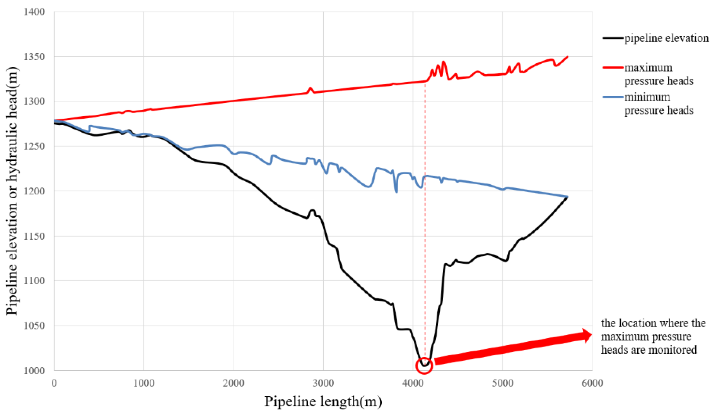
2.1. Study Area and Parameter Selection

In a gravity flow water supply project in Shanxi, the water is transported from a high-level storage tank (elevation: 1275.7 m, water level: 2.8 m) through a 5720 m pipeline, to an end storage tank (elevation: 1193.62 m, water level: 0 m). The flow and pressure regulating valve is installed in the end storage tank, and the valve closing time is 100 s. The pipe is a spiral steel pipe with a diameter of 250 mm, a wall thickness of 8 mm, an elastic modulus of 2.079 × 10¹¹ Pa and a friction factor of 0.012. The longitudinal section of the pipeline is shown in Figure 1. Although the height difference between the two storage tanks is small, the pipeline crosses the valley terrain with large undulations, which causes water hammer to easily occur. This gravity flow has characteristics such as a long distance, small pipe diameter, low flow and high drop, so it is valuable for analysis.

The parameters and reference values are shown in

Table 1. The initial value and range of each parameter.

Parameter Number	Parameter	Initial Value	Range
1	Valve closing time (s)	100.00	70.00~130.00
2	Flow rate (m3/s)	0.054	0.038~0.070
3	Friction factor	0.0249	0.0174~0.032
4	Young’s modulus of pipe (Pa)	2.079 × 1011	1.455 × 1011~2.703 × 1011
5	Pipe thickness (mm)	8.00	5.60~10.40
6	Pipe diameter (mm)	250.00	175.00~325.00

. According to the control equation, since the parameters do not affect each other, the local sensitivity analysis can meet the analysis requirements.

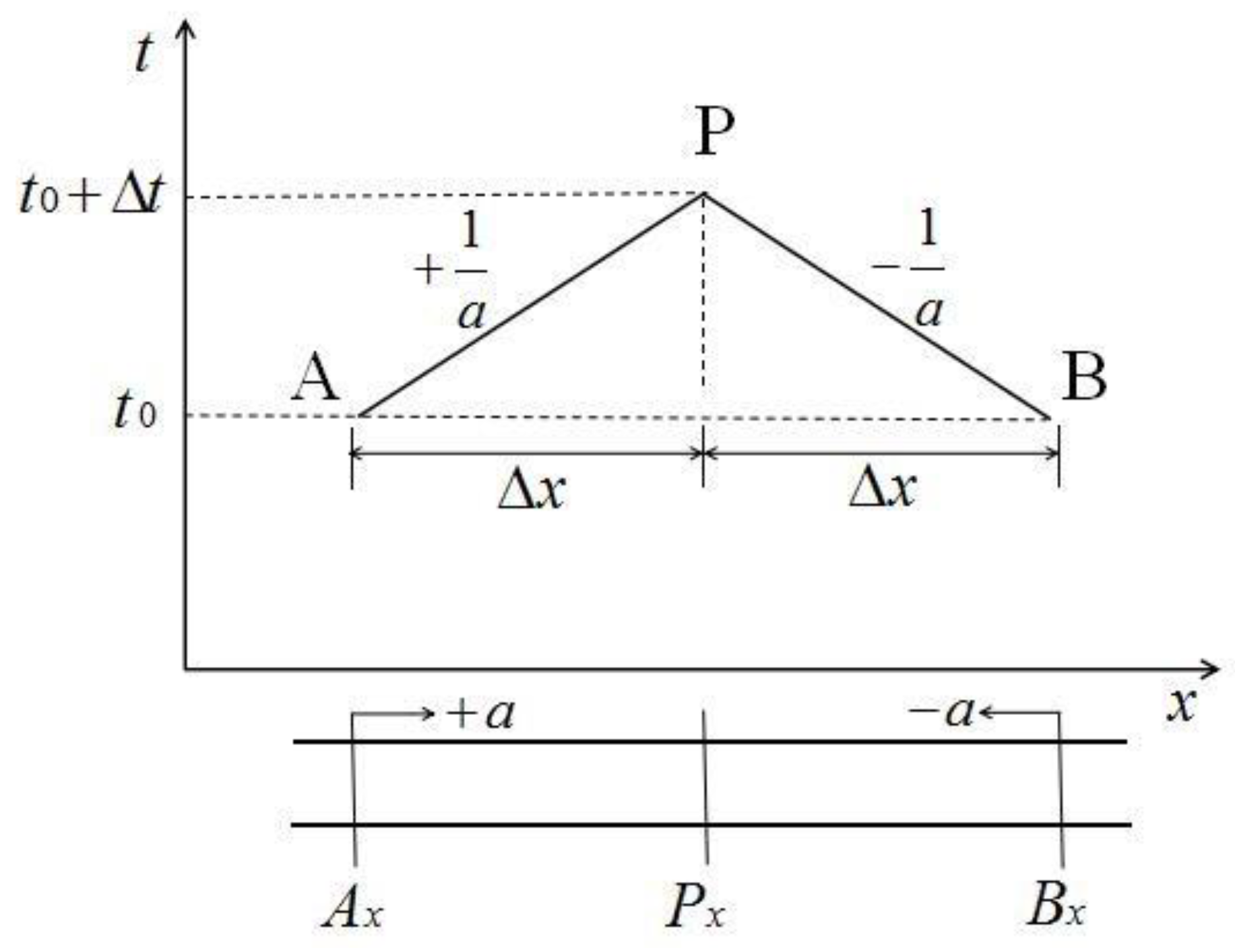
2.2. Control Equations and Calculation Methods

In the hydraulic transient simulation, the basic differential equation consists of two parts: the motion equation and the continuous equation.

$$\frac{\partial H}{\partial x}+\frac{1}{g}\frac{\partial V}{\partial t}+\frac{V}{g}\frac{\partial V}{\partial x}+\frac{2}{\rho R}{\tau }_w=0$$

(1)

$$\frac{\partial H}{\partial t}+V\left(\frac{\partial H}{\partial x}+\sin \alpha \right)+\frac{a^2}{g}\frac{\partial V}{\partial x}=0$$

(2)

The above equation is a set of partial differential hyperbolic equations from which it is difficult to obtain the analytical solution [3]. Based on the above introduction, the MOC is used to transform partial differential equations into ordinary differential equations. Since there is a detailed introduction about the MOC in the references, this paper only gives a brief introduction

$$\{\begin{array}{c}\frac{dV}{dt}+\frac{g}{a}\frac{dH}{dt}+\frac{2}{\rho R}{\tau }_w=0\\ \frac{dx}{dt}=+a\end{array}$$

(3)

$$\{\begin{array}{c}\frac{dV}{dt}-\frac{g}{a}\frac{dH}{dt}+\frac{2}{\rho R}{\tau }_w=0\\ \frac{dx}{dt}=-a\end{array}$$

(4)

The wall shear stress ${\tau }_w$ is the sum of two expressions [14]

$${\tau }_w={\tau }_q+{\tau }_u$$

(5)

where the ${\tau }_q$ calculated by using standard Darcy–Weisbach euqation

$${\tau }_q=\frac{f\rho V\left|V\right|}{8}$$

(6)

while the ${\tau }_u$ is expressed by the following convolution integral

$${\tau }_u=\frac{2\mu }{R}{\int }_0^{t}w\left(t-u\right)\frac{\partial v\left(u\right)}{\partial t}du$$

(7)

In the equation, μ is the dynamic viscosity, and w(t − u) is the weight function. To obtain the simplified format, integrate the above equation along the characteristic line

$$V_P-V_A+\frac{g}{a}\left(H_P-H_A\right)+\frac{2\Delta tf}{RA}{\tau }_{wA}=0$$

(8)

$$V_P-V_B-\frac{g}{a}\left(H_P-H_B\right)+\frac{2\Delta tf}{RA}{\tau }_{wB}=0$$

(9)

The two equations are straight lines with constant slopes, so the calculation process can be described by a rectangular grid. As shown in Figure 2, (Δx) is the spacing step length, the pipeline is evenly divided into (N) sections, (i) represents the order of each section, (i = 1) is the starting section and the terminal section is (i = N + 1). The calculation required is (Δt = Δx/a).

The calculation starts at (t = 0), given the parameters of points A and B, recursively, according to the time interval. Additionally, it obtains the parameter values of all grid nodes.

The boundary condition of the valve is

$$V=C_d\sqrt{2g\Delta H}$$

(10)

where C_d is the discharge coefficient, which depends on the valve performance curve and opening ratio τ at a specific time. In this study, the valve fully open flow coefficient C_d0 is 4731.

In the Equations (8) and (9), the calculation of the wave velocity adopts the elastic water hammer theory to calculate

$$a=\sqrt{\frac{K}{\rho }}\frac{1}{\sqrt{1+\frac{KD}{E\delta }}}$$

(11)

It can be seen from Equation (11) that the wave velocity α is related to the pipe diameter, wall thickness, Young’s modulus, fluid bulk elastic modulus and fluid density. In this study, the fluid is water, the bulk modulus is 1.96 × 10⁹ Pa and the density is 1000 kg/m³. Substituting Equation (11) for Equations (8) and (9), the calculation result is directly related to the pipe diameter, wall thickness and Young’s modulus, so that the parameters directly affect the calculation result.

2.3. Sensitivity Analysis Methods

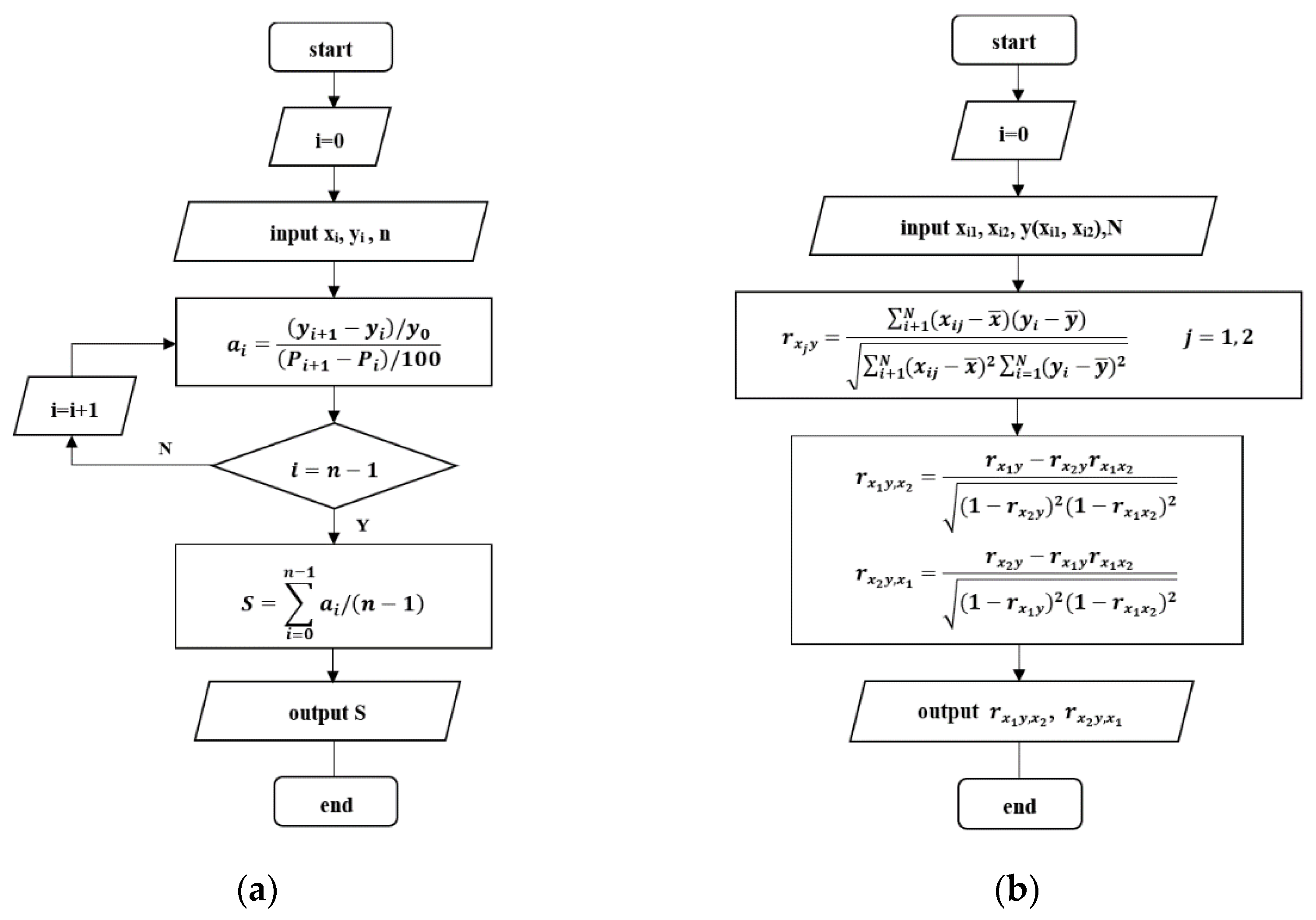
2.3.1. Morris Sensitivity Analysis

Morris sensitivity analysis [25] (also called Elementary Effects) can reflect the changes of the calculation results under the slight disturbance of factors. After a period of development [26], it has been widely used in sensitivity analysis. Morris adopts the concept of primary influence on factors, and the influence value of the i-th factor is expressed as

$$e_i=\frac{y\left(x_1,x_2,x_3,\dots ,x_i+\Delta ,\dots ,x_n\right)-y\left(x_1,x_2,x_3,\dots ,x_i,x_n\right)}{\Delta }$$

(12)

In the equation, suppose (x₁, x₂, x₃, …, x_n) are n input quantities that affect the output result of the model; (y) is the simulation output result of the model and (Δ) is the change quantity of the i-th input parameter.

Morris uses independent variables to change with a fixed step length, and the sensitivity discrimination factor takes multiple averages of Morris [22]

$$S={\displaystyle \sum }_{i=0}^{n-1}\frac{\left(y_{i+1}-y_i\right)/y_0}{\left(P_{i+1}-P_i\right)/100}/\left(n-1\right)$$

(13)

where (S) is the sensitivity judgment parameter, (y_i) is the output result of the i-th run of the calculation model, (y₀) is the reference value of the model parameter calculation result, (P_i) is the percentage of the change of the i-th model’s calculation parameter value to the reference value after the calibration parameter and (n) is the number of model runs.

The steps of Morris are shown in Figure 3a. According to the final calculation results, the sensitivity can be divided into four levels: ∣S∣ ≥ 1 (high-sensitivity parameter), 0.2 ≤ ∣S∣ < 1 (sensitivity parameter), 0.05 ≤ ∣S∣ 0 < 0.2 (medium sensitivity) and 0 ≤ ∣S∣ < 0.05 (not sensitive).

2.3.2. LHS-PRCC

PRCC is often combined with LHS for sensitivity analysis. By combining uncertainty analysis with PRCC, we can reasonably evaluate the sensitivity of our output variables to parameter changes.

LHS is a multi-dimensional stratified sampling method, which was first proposed by McKay et al. [27]. The advantage is that it requires fewer samples than simple random sampling to achieve the same accuracy. In LHS, parameters are randomly distributed in N equal probability intervals, and then the parameters are sampled. N represents the sample size. The choice of N should be at least k + 1, where k is the number of changing parameters, but usually much larger to ensure accuracy [28]. Because of its relatively uniform sampling, it has been widely used. The steps of LHS are as follows: first, the input ranges of each parameter are divided into N ranges with equal probability (N is the number of samples). Then, representative parameters are randomly selected from each divided range. Finally, these parameters are combined as a sampling result.

Partial correlation analysis is used to control the influence of other variables under the interaction of multiple variable factors and study the relationship between two specific variables [29]. The level of partial correlation analysis is determined by the number of research variables. The correlation coefficient (CC) between input x_j and output y is calculated as follows

$$r_{x_j,y}=\frac{{\sum }_{i+1}^N\left(x_{ij}-\overline{x}\right)\left(y_i-\overline{y}\right)}{\sqrt{{\sum }_{i+1}^N{\left(x_{ij}-\overline{x}\right)}^2{\sum }_{i=1}^N{\left(y_i-\overline{y}\right)}^2}} j=1,2,\dots ,k$$

(14)

The partial correlation coefficient (PCC) provides a measure of the strength of the linear relationship between input x_j and output y after eliminating the linear effects of other variables. The PCC between x_j and y is defined by the $r_{x_j,y}$ of ($x_j-{\widehat{x}}_j$) and ($y-\widehat{y}$), where ${\widehat{x}}_j$ and $\widehat{y}$ use the least square method to construct the regression model

$${\widehat{x}}_j=c_0+{\displaystyle \sum }_{\begin{array}{c}p=1\\ p\ne j\end{array}}^n{c}_p{x}_p,\widehat{y}=b_0+{\displaystyle \sum }_{\begin{array}{c}p=1\\ p\ne j\end{array}}^n{b}_p{x}_p$$

(15)

where (c₀, c₁, …, c_n) and (b₀, b₁, …, b_n) are coefficients determined in the construction of the regression model.

Similar to PCC, PRCC performs partial correlation on the rank transformed data; x_j and y are rank transformed first, and then the linear regression model described in the equation is performed. The value of PRCC ranges from −1 to +1, and the closer the absolute value |r| is to 1, the higher the correlation between the parameters; the closer it is to 0, the lower the correlation. The positive value of PRCC represents a positive correlation between the two parameters; on the contrary, the negative values represent a negative correlation.

In this study, the equation of the six parameters used is more complicated and detailed in the references [28,29]. Therefore, only the process of the two input parameters x₁, x₂ affecting the output parameter y is demonstrated in the Figure 3b flow chart of PRCC.

3. Results and Discussion

In this case, the main problem concerning gravity flow valve closing is controlling the maximum pressure in the hydraulic transient state so that the calculation results of the negative pressure do not change significantly. As a result, the maximum pressure is selected as the distinguishing parameter.

3.1. The Result of Morris

Based on the reference value of the model parameters, the MOC is used to analyze the local sensitivity of the hydraulic transient simulation results while the valve closes in gravity flow. The values of the parameters are perturbed with a fixed step of 10%, and the values are −30%, −20%, −10%, 10%, 20% and 30% of the reference value. According to the above calculation method, the maximum pressure value is calculated and recorded when the various parameters vary in different ranges. Then, the value of the sensitivity discrimination parameter S is calculated. The calculation results are shown in

Table 2. The sensitivity coefficient S and the level of each parameter.

Parameter Number	Parameter	S	Sensitivity Level
1	Valve closing time (s)	−0.242	Sensitivity parameter
2	Flow rate (m3/s)	0.347	Sensitivity parameter
3	Friction factor	0.020	Not sensitive
4	Young’s modulus of pipe (Pa)	0.006	Not sensitive
5	Pipe thickness (mm)	0.019	Not sensitive
6	Pipe diameter (mm)	−0.383	Sensitivity parameter

and Figure 4.

According to the parameter sensitivity coefficient, the sensitivity is as follows: the pipe diameter, flow rate, valve closing time, friction factor, pipe thickness and Young’s modulus of the pipe are in descending order. Among them, the pipe diameter, flow rate and valve closing time are all sensitive parameters; the friction factor, pipe thickness and Young’s modulus of the pipe are insensitive parameters. The valve closing time, Young’s modulus, friction factor and the maximum pressure are positively correlated; the pipe diameter, valve closing time, pipe wall thickness and the maximum pressure are negatively correlated.

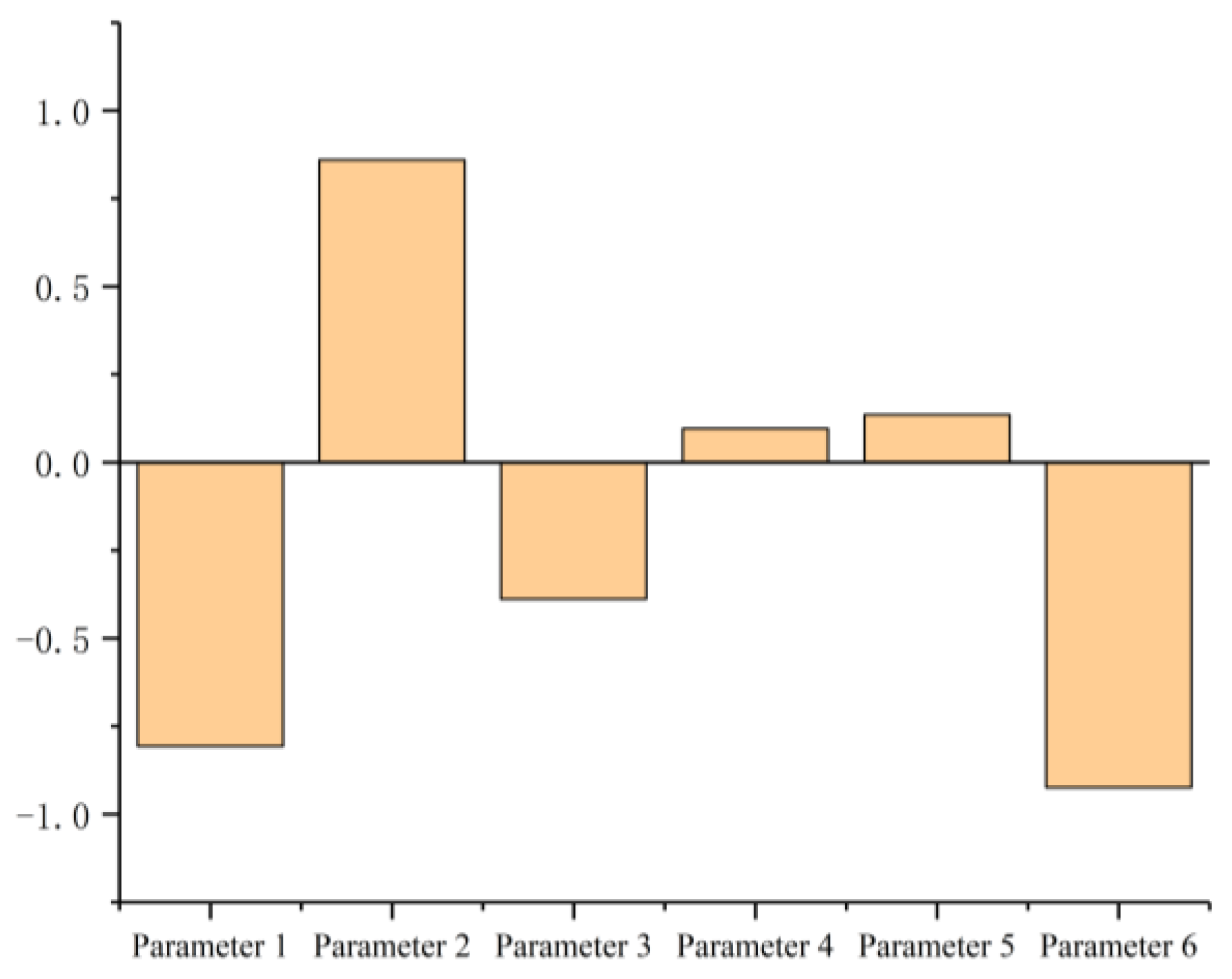
3.2. LHS-PRCC Analysis

In this study, we used the LHS to generate 25 sets of parameter samples from the range of each parameter given in Table 1 and performed hydraulic transient simulations. The parameter samples and maximum pressure calculation results are shown in

Table 3. The results of LHS.

Number	Valve Closing Time (s)	Flow Rate (m3/s)	Friction Factor	Young’s Modulus (Pa)	Pipe Thickness (mm)	Pipe Diameter (mm)	Maximum Pressure (m)
1	125.645	56.144	0.026	2.386 × 1011	7.681	283.788	296.841
2	127.826	38.052	0.031	2.244 × 1011	8.327	210.493	301.976
3	74.495	51.442	0.025	1.592 × 1011	9.572	298.601	319.967
4	115.808	48.514	0.022	1.973 × 1011	9.147	269.441	297.539
5	104.482	46.554	0.026	1.931 × 1011	6.336	200.200	327.434
6	93.766	63.972	0.027	2.636 × 1011	8.556	274.412	325.845
7	107.732	53.202	0.023	1.613 × 1011	8.814	187.536	358.472
8	119.087	61.940	0.022	1.775 × 1011	7.202	323.909	302.464
9	98.902	63.532	0.028	2.276 × 1011	7.004	227.417	342.644
10	84.484	44.062	0.019	2.008 × 1011	6.416	294.127	290.188
11	122.422	59.940	0.018	2.090 × 1011	9.929	222.184	332.570
12	89.271	65.280	0.030	1.667 × 1011	6.160	313.784	317.355
13	96.503	67.063	0.028	2.116 × 1011	5.940	261.522	328.255
14	102.435	44.252	0.023	1.536 × 1011	6.577	237.701	294.895
15	70.479	54.492	0.018	2.675 × 1011	9.795	246.130	351.802
16	84.059	42.327	0.020	2.549 × 1011	6.785	193.882	354.191
17	80.988	39.814	0.021	2.201 × 1011	8.953	309.268	288.788
18	113.402	49.666	0.021	2.577 × 1011	10.209	214.894	330.033
19	94.499	40.572	0.018	1.716 × 1011	9.425	255.921	302.486
20	122.897	47.827	0.018	1.808 × 1011	10.123	250.589	301.791
21	87.626	59.078	0.024	1.898 × 1011	8.268	282.544	321.346
22	77.114	55.254	0.020	2.475 × 1011	7.719	185.561	394.491
23	108.762	69.224	0.032	2.330 × 1011	8.095	180.260	365.335
24	77.358	67.849	0.029	2.453 × 1011	5.643	233.897	367.192
25	111.571	57.441	0.019	1.488 × 1011	7.363	305.560	303.349

.

According to the Latin hypercube sampling results in Table 3, the PRCC was calculated between each of the six parameters and the maximum pressure. Based on the magnitude of the absolute value of PRCC, the relative importance of the parameters is ranked. The PRCC calculation results of the parameters are shown in Figure 5 and

Table 4. The partial rank correlation coefficient r of each parameter.

Parameter Number	Parameter	r
1	Valve closing time (s)	−0.806
2	Flow rate (m3/s)	0.860
3	Friction factor	−0.388
4	Young’s modulus (Pa)	0.096
5	Pipe thickness (mm)	0.136
6	Pipe diameter (mm)	−0.924

.

PRCC analysis results show that the pipe diameter has the highest influence on the maximum pressure, followed by flow rate and valve closing time. The valve closing time, Young’s modulus and the maximum pressure are significantly positively correlated; on the other hand, the pipe diameter, valve closing time, friction factor, pipe wall thickness and the maximum pressure are negatively correlated.

3.3. Results Comparison and Discussion

3.3.1. Analysis of Parameters Related to Wave Velocity

In the gravity flow supply project, the maximum pressure generated by the water hammer increases with an increase in the wave speed. When the water hammer occurs due to cavity collapse, the trend of rising pressure is obvious; on the contrary, when the water hammer due to cavity collapse does not occur, the influence of the wave velocity on the maximum pressure is not obvious. The water hammer due to cavity collapse does not occur in this hydraulic transient simulation, so the Young’s modulus of the pipeline has a small, indirect effect on the maximum pressure by changing the wave velocity. The sensitivity analysis results of this simulation are consistent with previous research results, which is also an important reason for converting the wave velocity into other parameters for calculation in the second section. Among the parameters selected in this study, the parameters related to the wave velocity are the Young’s modulus, the pipe wall thickness and the pipe diameter.

From Equation (11), it can be seen that the Young’s modulus of the pipeline only indirectly affects the maximum pressure by changing the wave velocity. According to the calculation results, S₄ = 0.006 and r₄ = 0.096 (S is the Morris sensitivity parameter; r is the sensitivity parameter in LHS-PRCC). The maximum pressure increases with the increase in the Young’s modulus of the pipe. Moreover, its influence on the maximum pressure is small.

The reasons for the influence of pipe wall thickness and pipe diameter on the maximum pressure are similar: both come from the direct influence on the pipe flow area and the indirect influence on the wave velocity. The calculation result of the pipe wall thickness shows that S₅ = 0.019, r₅ = 0.136 and the pipe wall thickness has little effect on the calculation results. According to the parameter change range in Table 2, the maximum change of pipe wall thickness to pipe inner diameter is 2.40 mm, which is very small compared to the original pipe inner diameter of 243 mm. This makes the direct influence of pipe wall thickness on the maximum pressure small. Then, it has a small, indirect effect on the maximum pressure by influencing the wave velocity. Therefore, the pipe wall thickness is less sensitive to the maximum pressure. In the same way, the influence of pipe diameter on the maximum pressure mainly comes from the change of the water passing area. The maximum change of the pipe diameter to the inner diameter is 75.00 mm, so that the pipe diameter has a greater direct influence on the maximum pressure. The calculation result shows S₆ = −0.383 and r₆ = −0.924.

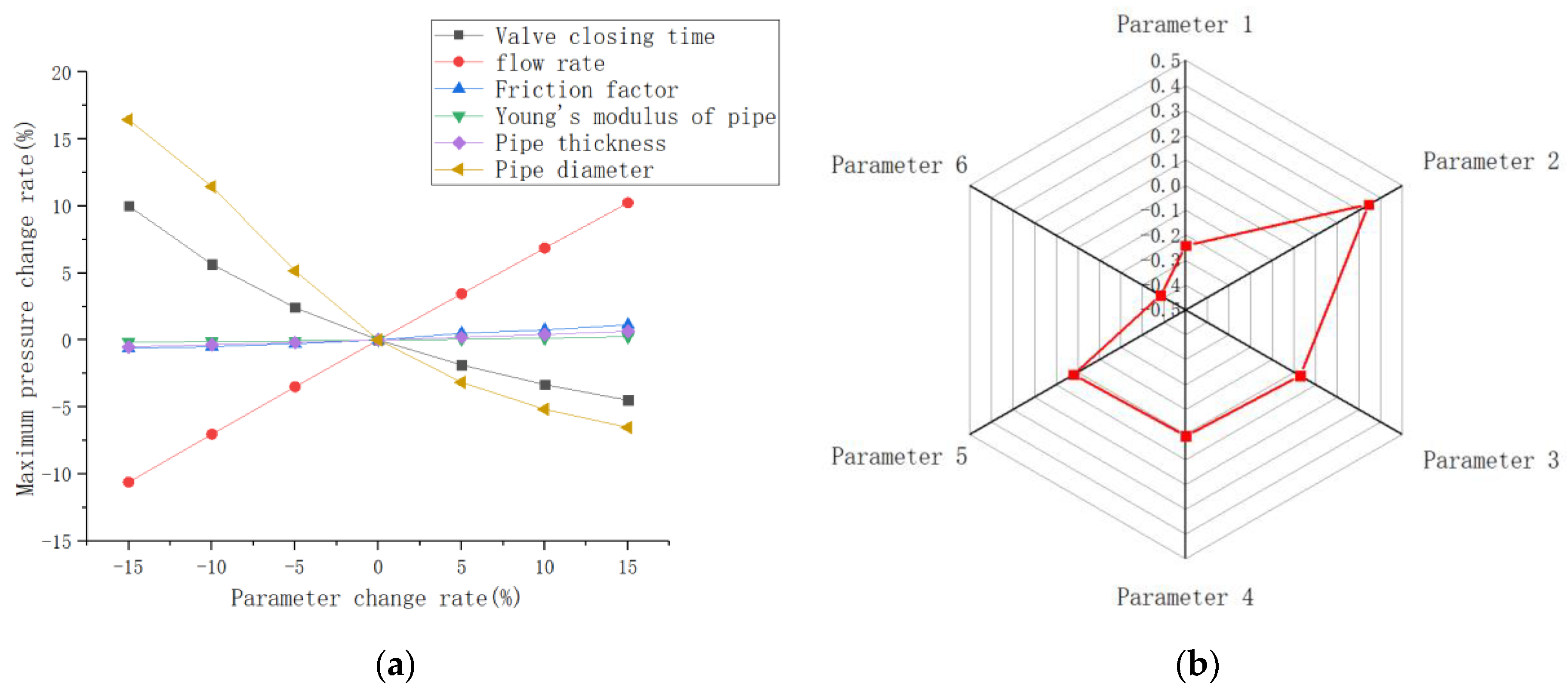
3.3.2. The Main Parameters That Affect the Maximum Pressure

According to the calculation results in Table 2 and Table 3, the pipe diameter, flow rate and valve closing time all have a significant impact on the maximum pressure, and the laws presented are basically the same. The results of the two methods can be mutually confirmed. The valve closing time directly determines whether direct water hammer or indirect water hammer occurs in the gravity flow water delivery system [5]. The result shows that S₁ = −0.242 and r₁ = −0.806. There are many related studies on the impact of valve closing time on the maximum pressure, and the results of this study are consistent with previous study results [9,30]. The result of the flow rate is S₂ = 0.347 and r₂ = 0.860. The values of the flow rate directly affect the pressure of the pipeline during steady-state operation. In the valve-closing hydraulic transient simulation, the change of the flow rate is the main reason for increasing the maximum pressure. Therefore, reducing the flow rate is also one of the commonly used measures in gravity flow water hammer protection. The analysis of the pipe diameter has been described in Table 2 and Table 3, and the result is S₆ = −0.383 and r₆ = −0.924.

According to the high sensitivity of these parameters in this simulation, they are the parameters that should be emphatically considered in hydraulic transient simulations. In the design of most water delivery projects in China, the selection of the pipeline diameter is often determined before the design of water hammer protection, and water hammer protection is only performed by adjusting the valve closing time, which is not conducive to the design of water hammer protection. Therefore, in the pipe diameter parameters of a water delivery project, the water delivery design and the water hammer protection design should be carried out at the same time, and the calculation results should be confirmed against each other to better complete the design of the water delivery project.

3.3.3. Analysis of the Variability of the Friction Factor in the Results

The correlation of the friction factor is different in the two methods. The increase in the friction factor will increase the head loss. Generally speaking, in a water supply project, the larger the friction factor of a pressurized pipeline, the smaller the flow rate and, thus, the safer the project. There are differences in the results of the two methods in this sensitivity analysis. The result shows that S₃ = 0.020 and r₃ = −0.388. In the two methods, the friction factor is not considered a more sensitive parameter. In the Morris sensitivity analysis, the maximum pressure increases with the increase in the friction factor; in LHS-PRCC, the maximum pressure decreases with the increase in the friction factor.

When the gravity flow water supply project is operating in the steady state, the flow is controlled by the flow and pressure regulating valve. When the friction factor of the pipeline increases and the water delivery capacity is sufficient, the water supply flow rate will not change due to the function of the flow and pressure regulating valve. When the transient process occurs, the increased friction reduces the amplitude of the water hammer wave fronts, leading to the line packing effect. This effect can cause a continuous pressure rise after the closure of the valve, and may produce overpressure [15]. This effect should be paid more attention to in high-friction pipes with long pipe lengths and small diameters. In the Morris analysis method, other parameters remain unchanged; only the friction factor is changed, resulting in a positive correlation between the friction factor and the maximum pressure. In LHS-PRCC, the parameters are all defined by stratified random sampling, and the changes of other parameters make the water supply capacity unable to be guaranteed. The line packing effect cannot be reflected under the changing parameter conditions. The friction factor will reduce the water transport capacity, resulting in a negative correlation between the friction factor and the maximum pressure.

In the similar gravity flow water supply projects with small pipe diameters and long distances, when the capacity of water delivery is sufficient and the friction factor of the pipeline increases, a bigger maximum pressure will be generated after the closure of the valve. In this case, more protection is required. This is what the design and operation managers need to pay more attention to.

4. Conclusions

In this study, the MOC was used in the gravity flow with obvious characteristics to carry out the hydraulic transient simulation. Then, the Morris screening method and LHS-PRCC were used to perform sensitivity analysis on calculations, and the following conclusions can be drawn:

• In this gravity flow example, the comparison of the two sensitivity analysis results shows that only some key parameters have an important influence on the calculation results. The sensitivity of key parameters from large to small are pipe diameter, flow rate and valve closing time. The friction factor, pipe thickness and Young’s modulus have little influence on the calculation results, and their sensitivity ranking has some variability.
• The simulation results have reference value for the design of similar gravity flow water delivery projects with obvious characteristics. In the design and operation of the project, the valve closing time, pipe diameter and flow rate should be strictly controlled to ensure the safety of the project.
• The sensitivity of the friction factor is different in the results of the two methods. After discussion, when other parameters remain unchanged, the maximum pressure increases with the increase in the friction factor due to the line packing effect; when other parameters change and the water delivery capacity cannot be guaranteed, the maximum pressure is negatively related to the friction coefficient. Therefore, more protective measures are needed when the friction factor of a gravity flow project becomes larger.
• The Morris screening method and LHS-PRCC gave similar parameter rankings for the selected parameters of the project in this case. The calculation results of the two methods are complementary in the sensitivity analysis of hydraulic transient simulation. At the same time, this study also confirms the applicability of the two methods in the sensitivity analysis of hydraulic transient simulations.

In summary, in this study, we analyzed the parameter sensitivity of hydraulic transient simulations based on the MOC in gravity flow. We only analyzed one engineering example, which proved the applicability of the two sensitivity analysis methods. In order to obtain more comprehensive results, more examples need to be analyzed.

References

1. Wang, R.; Wang, Z.; Wang, X.; Yang, H.; Sun, J. Pipe Burst Risk State Assessment and Classification Based on Water Hammer Analysis for Water Supply Networks. J. Water Res. Plan. Manag. 2014, 140, 4014005. [Google Scholar] [CrossRef]
2. Yang, K. Review and frontier scientific issues of hydraulic control for long distance water diversion. J. Hydraul. Eng. 2016, 47, 424–435. (In Chinese) [Google Scholar] [CrossRef]
3. Abdeldayem, O.; Ferràs, D.; van der Zwan, S.; Kennedy, M. Analysis of Unsteady Friction Models Used in Engineering Software for Water Hammer Analysis: Implementation Case in WANDA. Water 2021, 13, 495. [Google Scholar] [CrossRef]
4. Wylie, E.B.A.S. Fluid Transients; McGraw-Hill: New York, NY, USA, 1978; p. 384. [Google Scholar]
5. Chaudhry, H.M. Applied Hydraulic Transients; Van Nostrand Reinhold: New York, NY, USA, 1987; p. 521. [Google Scholar]
6. Wylie, E.B.; Streeter, V.L.; Lyle, V.; Suo, L. Fluid Transients in Systems; Prentice Hall: Hoboken, NJ, USA, 1993; p. 463. [Google Scholar]
7. Kwon, H.J.; Lee, J. Computer and Experimental Models of Transient Flow in a Pipe Involving Backflow Preventers. J. Hydraul. Eng. 2008, 134, 426–434. [Google Scholar] [CrossRef]
8. Han, S.Y.; Hansen, D.; Kember, G. Multiple scales analysis of water hammer attenuation. Q. Appl. Math. 2011, 69, 677–690. [Google Scholar] [CrossRef] [Green Version]
9. Kou, Y.; Yang, J.; Kou, Z. A Water Hammer Protection Method for Mine Drainage System Based on Velocity Adjustment of Hydraulic Control Valve. Shock Vib. 2016, 2016, 1–13. [Google Scholar] [CrossRef] [Green Version]
10. Tian, W.; Su, G.H.; Wang, G.; Qiu, S.; Xiao, Z. Numerical simulation and optimization on valve-induced water hammer characteristics for parallel pump feedwater system. Ann. Nucl. Energy 2008, 35, 2280–2287. [Google Scholar] [CrossRef]
11. Bettaieb, N.; Taieb, E.H. Assessment of Failure Modes Caused by Water Hammer and Investigation of Convenient Control Measures. J. Pipeline Syst. Eng. 2020, 11, 4020006. [Google Scholar] [CrossRef]
12. Afshar, M.H.; Rohani, M.; Taheri, R. Simulation of transient flow in pipeline systems due to load rejection and load acceptance by hydroelectric power plants. Int. J. Mech. Sci. 2010, 52, 103–115. [Google Scholar] [CrossRef]
13. Urbanowicz, K. Modern Modeling of Water Hammer. Pol. Marit. Res. 2017, 24, 68–77. [Google Scholar] [CrossRef]
14. Urbanowicz, K.; Stosiak, M.; Towarnicki, K.; Bergant, A. Theoretical and experimental investigations of transient flow in oil-hydraulic small-diameter pipe system. Eng. Fail. Anal. 2021, 128, 105607. [Google Scholar] [CrossRef]
15. Liou, J.C.P. Understanding Line Packing in Frictional Water Hammer. J. Fluids Eng. 2016, 138, 081303. [Google Scholar] [CrossRef]
16. Ionescu-Bujor, M.; Cacuci, D.G. A Comparative Review of Sensitivity and Uncertainty Analysis of Large-Scale Systems—I: Deterministic Methods. Nucl. Sci. Eng. 2004, 147, 189–203. [Google Scholar] [CrossRef]
17. Cacuci, D.G.; Ionescu-Bujor, M. A Comparative Review of Sensitivity and Uncertainty Analysis of Large-Scale Systems—II: Statistical Methods. Nucl. Sci. Eng. 2004, 147, 204–217. [Google Scholar] [CrossRef]
18. Yi, X.; Zou, R.; Guo, H. Global sensitivity analysis of a three-dimensional nutrients-algae dynamic model for a large shallow lake. Ecol. Model. 2016, 327, 74–84. [Google Scholar] [CrossRef]
19. Ouatiki, H.; Boudhar, A.; Ouhinou, A.; Beljadid, A.; Leblanc, M.; Chehbouni, A. Sensitivity and Interdependency Analysis of the HBV Conceptual Model Parameters in a Semi-Arid Mountainous Watershed. Water 2020, 12, 2440. [Google Scholar] [CrossRef]
20. Xu, X.; Sun, C.; Huang, G.; Mohanty, B.P. Global sensitivity analysis and calibration of parameters for a physically-based agro-hydrological model. Environ. Model. Softw. 2016, 83, 88–102. [Google Scholar] [CrossRef] [Green Version]
21. Li, C.; Wang, W.; Xiong, J.; Chen, P. Sensitivity Analysis for Urban Drainage Modeling Using Mutual Information. Entropy 2014, 16, 5738. [Google Scholar] [CrossRef]
22. Wan, W.; Huang, W.; Li, C. Sensitivity Analysis for the Resistance on the Performance of a Pressure Vessel for Water Hammer Protection. J. Press. Vessel. Technol. 2014, 136. [Google Scholar] [CrossRef]
23. Wan, W.; Li, F. Sensitivity Analysis of Operational Time Differences for a Pump–Valve System on a Water Hammer Response. J. Press. Vessel. Technol. 2016, 138. [Google Scholar] [CrossRef]
24. Zhu, Y.Z.Y.; Zhang, J.Z.J.; Hu, M.H.M. Random model of water hammer pressure and probability analysis in waterpower station. In Proceedings of the ASME/JSME 2007 5th Joint Fluids Engineering Conference, San Diego, CA, USA, 30 July–2 August 2007; pp. 47–55. [Google Scholar]
25. Morris, M.D. Factorial Sampling Plans for Preliminary Computational Experiments. Technometrics 1991, 33, 161–174. [Google Scholar] [CrossRef]
26. Ge, Q.; Menendez, M. Extending Morris method for qualitative global sensitivity analysis of models with dependent inputs. Reliab. Eng. Syst. Saf. 2017, 162, 28–39. [Google Scholar] [CrossRef]
27. Mckay, M.D.; Beckman, R.J.; Conover, W.J. Comparison of 3 methods for selecting values of input variables in the analysis of output from a computer code. Technometrics 1979, 21, 239–245. [Google Scholar]
28. Marino, S.; Hogue, I.B.; Ray, C.J.; Kirschner, D.E. A methodology for performing global uncertainty and sensitivity analysis in systems biology. J. Theor. Biol. 2008, 254, 178–196. [Google Scholar] [CrossRef] [PubMed] [Green Version]
29. Helton, J.C.; Davis, F.J. Illustration of sampling-based methods for uncertainty and sensitivity analysis. Risk Anal. 2002, 22, 591–622. [Google Scholar] [CrossRef] [PubMed]
30. Yao, E.; Kember, G.; Hansen, D. Analysis of Water Hammer Attenuation in Applications with Varying Valve Closure Times. J. Eng. Mech. 2015, 141, 4014107. [Google Scholar] [CrossRef]
Figure 1. Pipeline elevation trend and envelopes of maximum and minimum pressure heads for the case with initial values.
Water 13 03464 g001
Figure 2. The characteristic lines of the MOC.
Water 13 03464 g002
Figure 3. The flow charts of two sensitivity analysis methods: (a) the flow chart of Morris; (b) the flow chart of PRCC.
Water 13 03464 g003
Figure 4. Sensitivity analysis results of Morris: (a) the change rate of the maximum pressure caused by parameter disturbance; (b) sensitivity parameter S radar chart.
Water 13 03464 g004
Figure 5. Comparison analysis chart of LHS-PRCC r results.
Water 13 03464 g005