1. Introduction
1.1. General Overview
In the Dutch Rhine-Meuse delta river embankments, including dikes to reinforce natural levees, form an essential part of the primary flood defence. One of several key mechanisms threatening the stability of dikes is piping [
1,
2,
3,
4,
5,
6]. For this process, the occurrence of pervious layers overlain by impervious cover layers is of concern [
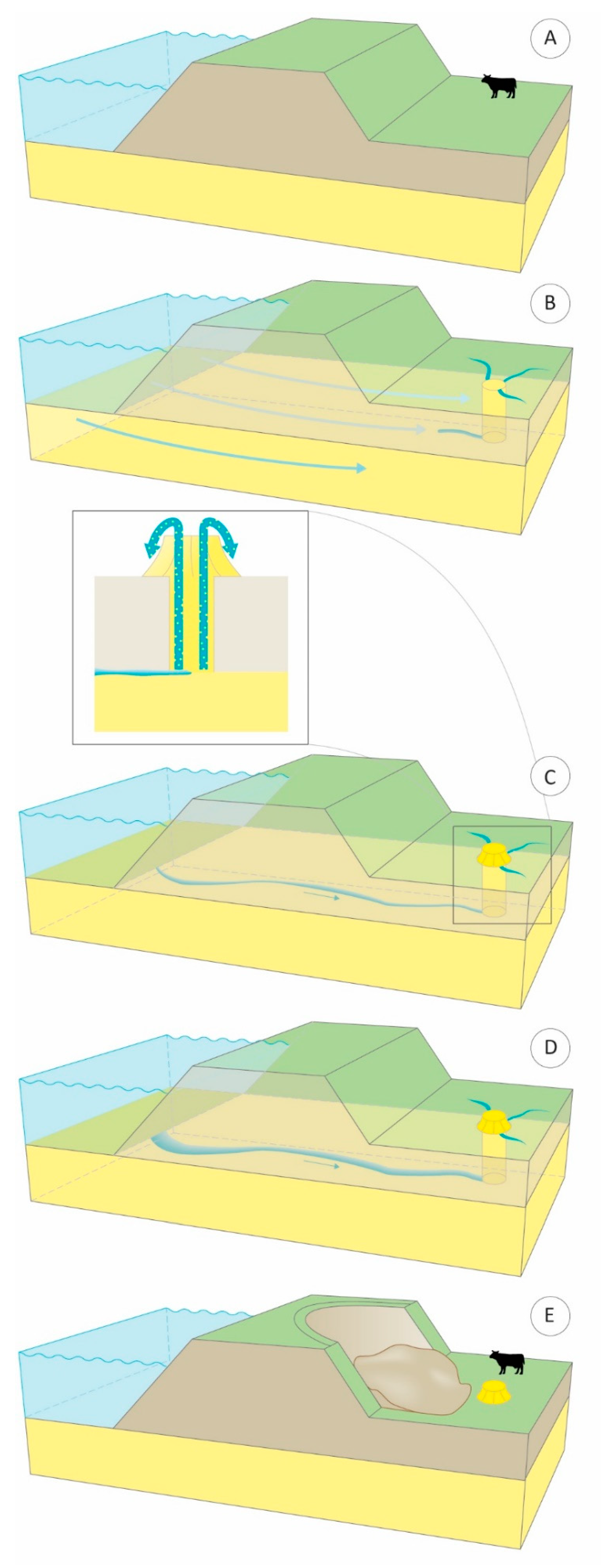
7]. The impervious cover layer prevents pressure and water from being released over wider areas (due to seepage), causing a concentration of flow to a single exit point which either occurs naturally or through engineering works that compromise the integrity of the cover layer (see
Figure 1).The hydraulic gradient between the river and the seepage point can be of sufficient magnitude to entrain sand particles in the underlying pervious layer, particularly during high river stages. The entrained sand can subsequently be expulsed from the outflow point, initiating backward erosion. When allowed to continue progressing upstream, this could eventually lead to a slump type failure in an overlying embankment [
5,
8,
9].
The Rhine-Meuse delta is characterised by alluvial deposits formed by a highly complex past of many avulsions and changing sedimentary environments [
10]. This has led to a highly heterogeneous subsurface of intersecting or overlapping channel belts that have no bearing on the present-day topography and hydrography. Due to differences in facies, channel belts are characterized by lateral and vertical lithological transitions and short-range shifts in facies and texture classes [
11]. This in turn creates a complex hydrogeological setting [
12,
13]. Thus, it is essential to consider subsurface variability underneath embankments in relation to piping [
14].
1.2. Research Objectives
Therefore, this paper aims to quantify empirically the dependence of the initiation gradient for backward erosion on the particle size distribution. To this end, small-scale laboratory experiments were performed in which different mixtures of sands and fines were combined and subjected to increasing hydraulic gradients until piping started. The results of these experiments can be interpreted in terms of the imposed gradients. In combination with the permeability of the sand-fines mixture, the resulting groundwater flow and the associated buoyant and drag forces leading to the entrainment of particles and progressive upstream extension of the pipes are imposed. By varying the grain size distribution, whilst maintaining the same D70, it is possible to isolate the influence of the shape of the grain size on the piping process. Hereby the choice to maintain the same D70 between different samples is based on the currently most prevalent method of determining piping risk, the Sellmeijer method, which uses the D70 percentile [
15,
16] to include the influence of grain size. This empirical evidence will provide the basis for further model development and the design of laboratory experiments by which hypotheses on the nature of pipe erosion can be tested. Specifically, the experiments described here were designed to:
Relate the flow velocity to particle entrainment by means of Stokes’ Law;
Identify the critical gradient for initiation of backward erosion;
Establish a relationship between particle size distribution and bulk permeability;
1.3. Subsurface Parameters
In areas with heterogeneous alluvial deposits, the occurrence of piping is, for a large part, dependent on the hydrogeological setting. On a regional scale, the subsurface heterogeneity and the resulting hydrological setting precondition the occurrence of piping and sand boils [
6,
14,
17,
18,
19,
20]. On a local scale, the formation of pipes is directly linked to the particle size distribution, which in itself is linked to the larger scale heterogeneity defined by the channel belt architecture. At present, methods to assess the risk of piping focus on its critical gradient for progression and employ the hydraulic gradient to capture the regional setting and include the local material properties through a measure for intrinsic permeability, and a deviation from a characteristic particle size, relative density and uniformity coefficient [
15,
16,
21,
22]. These parameters were chosen based on their availability in relation to previous research on piping. Careful consideration must be made for each of the aforementioned methods to describe piping risk [
16,
23,
24] in regards of which process is being described by these methods. None of these methods consider the conditions for the initiation of the pipe, merely its ability to progress upstream.
Specifically, the influence of these parameters on the piping process can be related to two sub-processes: first, in terms of the flow velocities that are the product of subsurface permeability and hydraulic gradient-; and second: the pipe developing as particles are entrained by the flow and grows against the direction of stream. As flow converges in the ever-growing pipe, the grain size and flow velocity in the pipes being the determining factor if the pipe is able to progress in terms of erodibility [
15,
16,
22,
24,
25,
26,
27]. In the former, permeability is influenced by the grain size distribution of the medium in which the process takes place: particle packing, infilling, and tortuosity determine the permeability and porosity [
26,
28,
29]. Given the hydraulic gradient, the permeability determines the specific discharge and thus, with the porosity, the Darcian and pore flow velocities of water passing under the dike. In the latter case, drag forces exerted on the grains from upward flow to the exit point of a pipe determine if the grains are able to be transported to the surface elevation and be expulsed.
The associated hydraulic gradient in this paper is referred to as the initiation gradient (defined as Hi/L, head difference (Hi) over the flow path length (L)). This is the onset of backward erosion piping. Once a pipe is forming, the created space will funnel flow and enhance the uptake of particles, leading to a positive feedback loop. At this point either the increasing length and width of the pipe can cause the flow velocity in the pipe to decrease to a magnitude insufficient for sediment transport; or the hydraulic gradient remains large enough for the pipe to continue to grow. The latter is the critical hydraulic gradient (referred to as Hc/L, head difference (Hc) over the flow path length (L)).
1.4. Applicability of the Grain Size Distribution
The particle size distribution defines a representative elementary volume for which the groundwater flow and the resulting buoyant forces and drag forces it exerts can be described effectively, which is amenable to laboratory experiments to study the initiation of pipes under controlled conditions. The particle size distribution is the representation of heterogeneity at the finest scale that can be included in hydrological and geotechnical models to predict piping in the shape of its parameters and tensors [
13,
26]. The particle size distribution thus occupies a central role in the prediction of piping as it connects the regional geological setting, to which it is genetically linked, to the field scale at which the particle size distribution can be adequately sampled, thus providing potentially a predictive model of relevant subsurface conditions [
10,
30]. In order to further our understanding on the initiation of pipes, it is essential to separate the hydrological and mechanical influences of the particle size distribution and to consider its entire range, compared to the more reduced measures of particle size distribution
1.5. Relative Flow Velocity
Once the grain size distribution is known it can be used to relate various observed hydraulic gradients and flow velocities to the initiation of backward erosion for different grain size diameters. One method is by relating the conditions for liquefaction of the medium to the moment initiation of backward erosion [
20]. Hereby the upward forces (buoyancy and fluid-induced drag force) on a grain outbalance the downward forces (gravity). Solving this for relative vertical fluid flow velocity gives Stokes’ Law for terminal settling velocity [
31]. As per this law, in the vertical outflow channel, the velocity of the fluid relative to the particles for no net forces on an individual sand particle can be described as shown in Equation (1).
Here is the dynamic viscosity (Pa∙s), υ (ms−1) is the flow velocity relative to the grain, g is the gravitational acceleration (ms−2), and (kg m−3) are the densities of the particles and the fluid respectively and R [m] is the radius of the particles. Assuming that the pipe is about to form (i.e., the very first grains are able to be eroded and transported) the controlling factors would thus be the flow velocity and the size of the particles to be transported as the friction between particles is neglected in this approach. This implies that the outflow point of the pipe already exists, which can be described as a vertical channel through the cover layer. Thus, flow velocity only occurs in the vertical direction. As the friction between grains is ignored, this approach is only valid for particles at the very top which are lying freely upon the matrix. Still, the method captures the forces that are required in order to initiate piping as a conservative estimate.
2. Materials and Methods
2.1. Particle Size Distributions
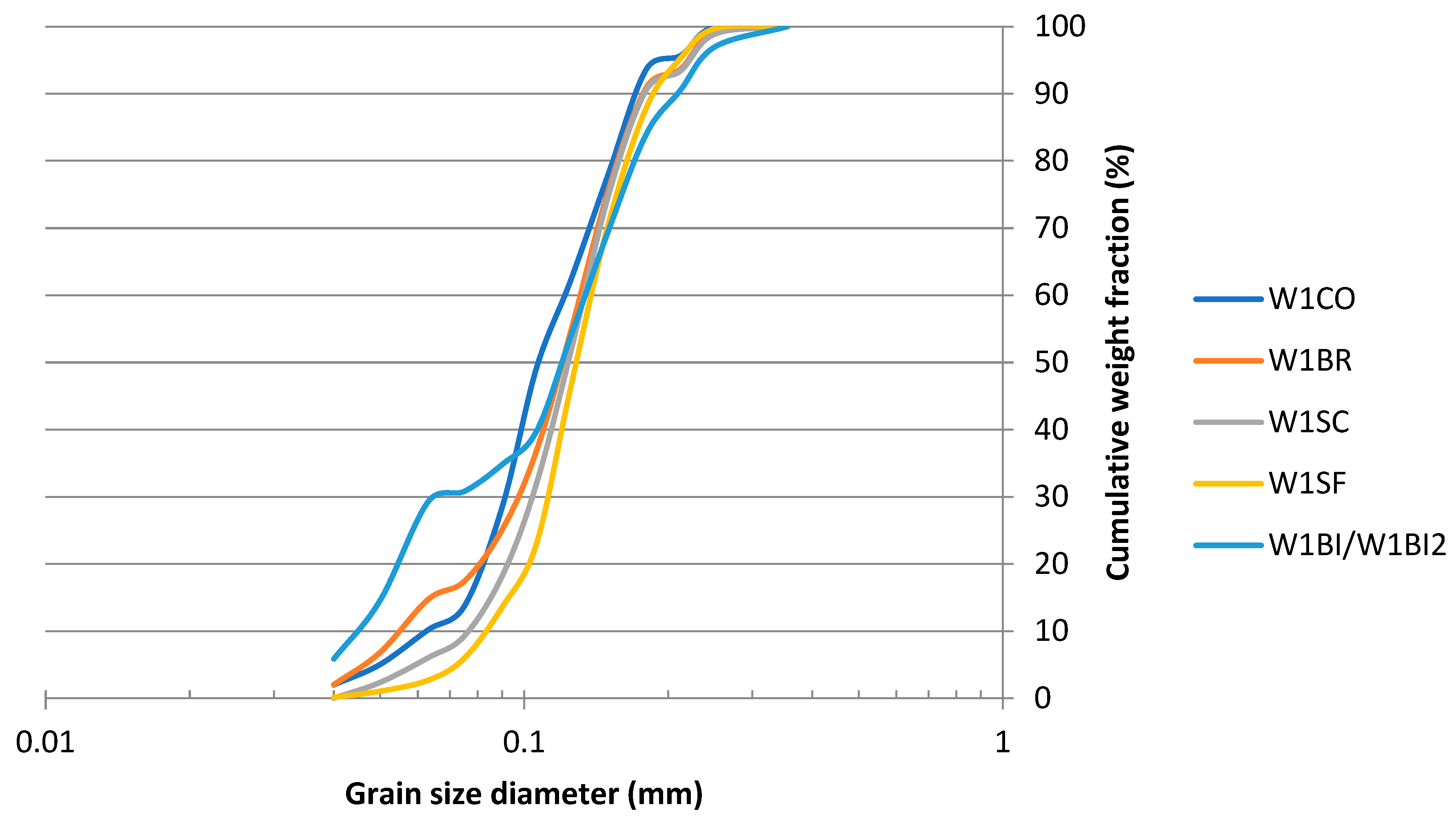
To investigate the influence of the particle size distribution on the initiation and progression of pipes, five different sand-fines mixtures were subjected to critical groundwater flow velocities under controlled laboratory conditions at the facilities at Deltares in Delft (The Netherlands). The samples were different in the particle size distribution but had a comparable D70 around 150 µm, given the central role of this index in practical methods to estimate the hazard of piping under dikes as indicated by e.g., the Sellmeijer method [
15]. The grain size distributions of the used sand samples are depicted in
Figure 2, and the exact properties are displayed in
Table 1. W1CO, the control experiment, used and almost uniform and narrow grain size distribution, whereas the distribution of W1BR was wider. W1SC was skewed towards the broader fraction, W1SF was skewed towards the finer fraction, W1BI2 and W1BI were the broadest grain size distributions tested and have the same grain size distribution, as W1BI2 was repeated due to this sample not exhibiting backward erosion piping. These were added to and used conjointly with a database of similarly configured experiments. For this database, see
Appendix A.
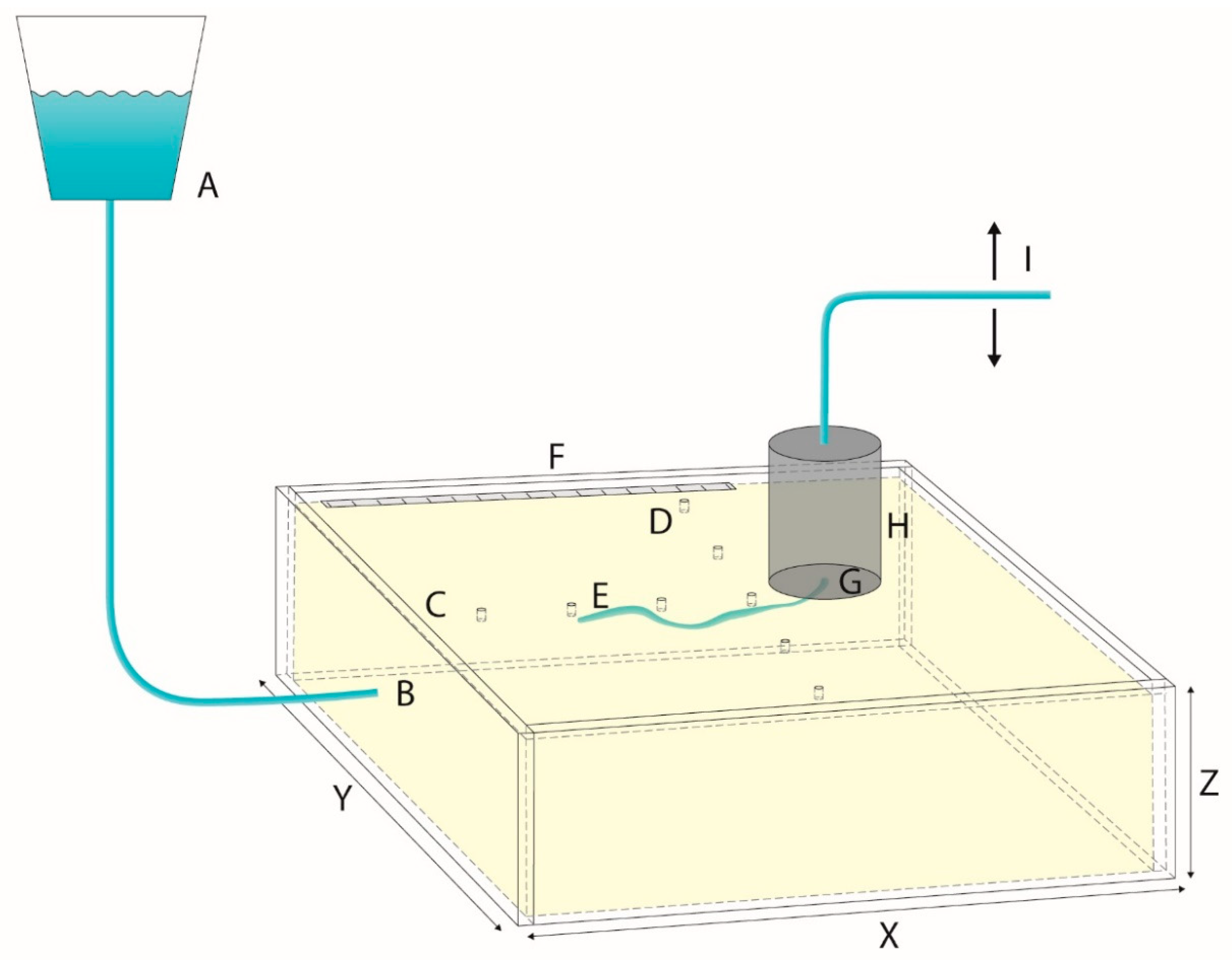
2.2. Box Experiment Configuration and Preparation
The experimental setup consisted of a box in which a sand sample was placed and confined with an acrylic glass plate. In the acrylic top plate, the only outflow point during the experiment was provided by a hole with a diameter of 6 mm that was located in the centre of the acrylic plate at a distance of 344 mm (L) from the inlet side at the upper end of the box and 139 mm from its lower end. The internal dimensions of the box were 483 mm long, 301 mm wide, and 101 mm deep. The confined sample was subjected to a positive head difference between an inlet at the upper side of the box and the outflow point. This inlet was 200 mm wide and extended the full depth of the box and was positioned centrally on that side. The ensuing gradient between the inlet and the outlet resulted in Darcian flow, and the gradient was increased gradually until the water at the outlet washed out particles from the sample. This gradient was considered to be just above the initiation gradient, the critical magnitude required to expulse sediment and initialize pipe erosion. The backward extension of the pipe from the outlet upwards could be monitored and photographed through the acrylic glass plate. This filter served as the inlet of water for the sample that was fully saturated. At the lower end, on the opposite side of the sample, a circular stone filter sat at the end of the box and provided a possible drain to, for example, release overpressure, this filter was closed during the experiment. The impervious base underneath the sample is used as datum (z = 0), and gradients are defined relative to this.
Open stand pipes to measure the hydraulic head are placed in the acrylic plate, sides and bottom of the box. Along the centre line of the box, 5 open stand pipes were inserted through the acrylic plate at regular intervals and complemented with 4 open standpipes that ran perpendicularly to this row across the outlet. Three more open stand pipes were placed at regular intervals in the bottom of the box and three more along the length of the box. In addition, an open stand pipe was placed at respectively the inlet and the outlet to observe the gradient over time. This gradient was imposed as the difference in the constant head imposed by two overflowing reservoirs at the inlet and the outlet respectively. A head difference was created by lowering the head of the outlet below that at the inlet. An additional recipient was placed around the outlet to catch the expulsed sediment. Since this cylindrical recipient had a much larger diameter than the outflow point, the flow velocity would decrease in the sediment, causing the expulsed sample to settle there.
The procedure to place the sample in the box involved holding the box vertically with the inlet side at the bottom, removing the plate at the top. Throughout the filling of the box, dry sample was poured gently into a shallow layer of degassed water so no air would get trapped between the particles. Pouring was done at a consistent and low rate in order to prevent splashing that would cause air to enter the water and create excessively large voids. The water level was kept as shallow as possible to prevent the particles from the particles settling differentially as a result of the varying fall velocities. Once filled, the excess material was scraped off and the top was closed off with a watertight seal by screwing the top side back on. After this, the container was placed horizontally so the acrylic plate would be on the top (See
Figure 3). The saturated material was then allowed to rest for 24 h during which any excess water could drain and allow the container to lose overpressure before the experiment was started.
2.3. Box Experiment Execution
At the start of the experiment, the two reservoirs that maintained the constant head at the inlet at the upper side of the sample and at the outlet in the confining plate were placed at an equal elevation of 1000 mm above the base. As there was no difference between them, the gradient was zero but a positive, hydrostatic pore pressure of 1000 mm existed at the base of the sample. At the top of the sample, the elevation head was 101 mm and the pore pressure consequently 899 mm. During the experiment the constant head reservoir at the outlet was gradually lowered, thus creating the gradient that leads to groundwater flow and changing the pore pressure distribution in the box. The lowering continued with increments of 5 mm per 5 min until erosion started and the incipient formation of a pipe was noticed below the acrylic glass plate. With each increment, the discharge through the exit point was measured by diverting the outflow of water into a container for a set amount of time and determining the volume per time unit. Using the principles of continuity of flow this can be used to reconstruct the average flow velocity in the box in different slices. Initiation of backward erosion, rather than just the boiling of finer sediment at the outflow point was taken as a reference point for pipe initialisation for determining the hydraulic gradient. This is different from some experiments available in the compiled database, which take the first occurrence of the boiling of sand as the starting point. As long as backward erosion continued, the gradient was kept constant, but it was increased further when the pipe stabilised in order to keep erosion going. When the pipe reached the inlet filter the experiment was stopped and the head required for this to occur was noted as the critical gradient for backward erosion.
2.4. Hydraulic Parameters
Relevant parameters, such as porosity and saturated conductivity, were determined from the sample respectively before and after the test. Porosity was determined using the dry bulk mass of the sample and the particle density to determine the volume of the solids for the total volume of the experiment box. Saturated conductivity was determined from the drop in hydraulic head through the experiment prior to the occurrence of backward erosion and the measured discharge, combined with the assumption of continuity of flow. Discharge was determined at the outflow point of the experimental set up by diverting the outflow into a measuring cup for a predetermined amount of time, allowing for a direct determination of discharge in volume per time unit. Dividing by area of the outflow point resulted in the flow velocities in
Table 2. In order to relate the saturated conductivity to the particle size distribution and the uniformity coefficient, representative subsamples were analysed by dry sieving. For the experiments available in the database, the saturated hydraulic conductivity was fitted given the imposed gradient and the observed flow assuming Darcian flow prior to disturbance of the sample by erosion.
3. Results
3.1. Initiation Gradient and Flow Velocity
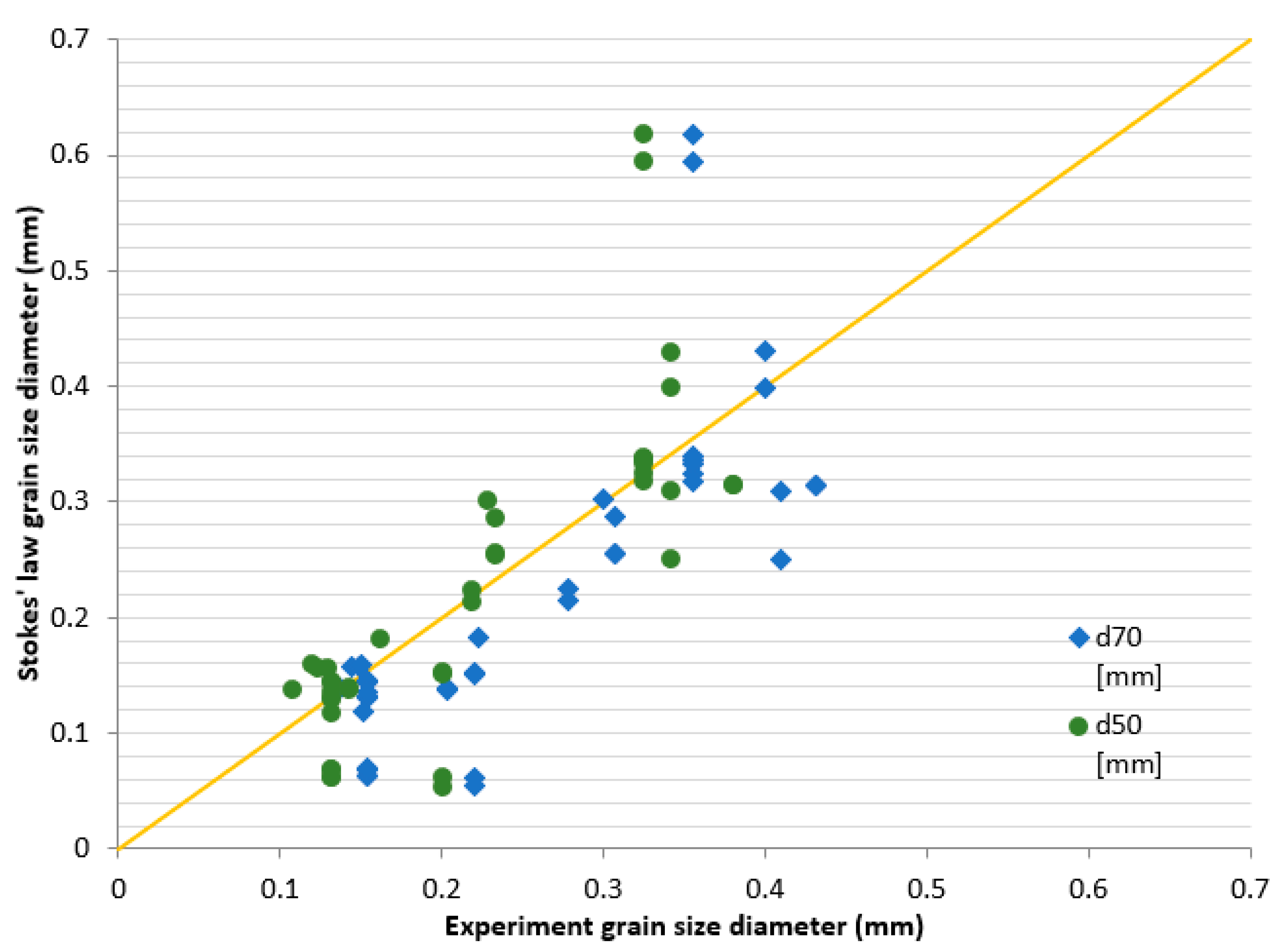
Using Stokes’ law, the flow velocity measured in the vertical channel at the initiation gradient for backward erosion was used to determine the grain size for which the upward and downward forces balance out. Comparing this to the grain sizes of the actual samples show that Stokes’ law performed quite well, as shown in
Figure 4, which combines the results of this experiment series (
Table 2) with the results of previous studies (
Appendix A). The D50 performed slightly better than the D70 for predicting the flow velocity required to initiate backward erosion. However, the differences between D50 and D70 for the samples used was quite small and results are therefore very similar. Thus, unless the grain size distribution is exceptionally broad, both D50 and D70 can be used as an indicator for predicting the velocity required to initiate backward erosion, especially for smaller grain sizes.
The results in
Figure 4 thus show that using Stokes’ law to determine the velocity, as a function of permeability, at which a grain can be transported is a valid method across a long range of samples, which indicates that an accurate assessment of flow velocity as a function of hydraulic gradient and saturated conductivity is paramount for predicting the moment of initiation of backward erosion. Further results of the experiment are shown in
Table 2, which depicts the critical hydraulic head gradients at which backward erosion starts. It also lists the associated measured flow velocity at the outflow point and the settling velocity estimated with Stokes’ law Equation (1). Two notable outliers are present, which did not exhibit typical piping behaviour and are thus not further considered in this study. Flow through sample W1BR behaved as non-linear flow and sample W1BI2 exhibited forward erosion.
3.2. Hydraulic Conductivity and Grain Size Distribution
The suitability of Stokes law to predict the initiation of transport of particles, indicates that, in order to determine the gradient required to initiate backward erosion outside of these experiments, a description of saturated conductivity is required. Therefore, we also investigated estimated hydraulic conductivity from grain size parameters of our experiments. In line with previous research reported by Odong [
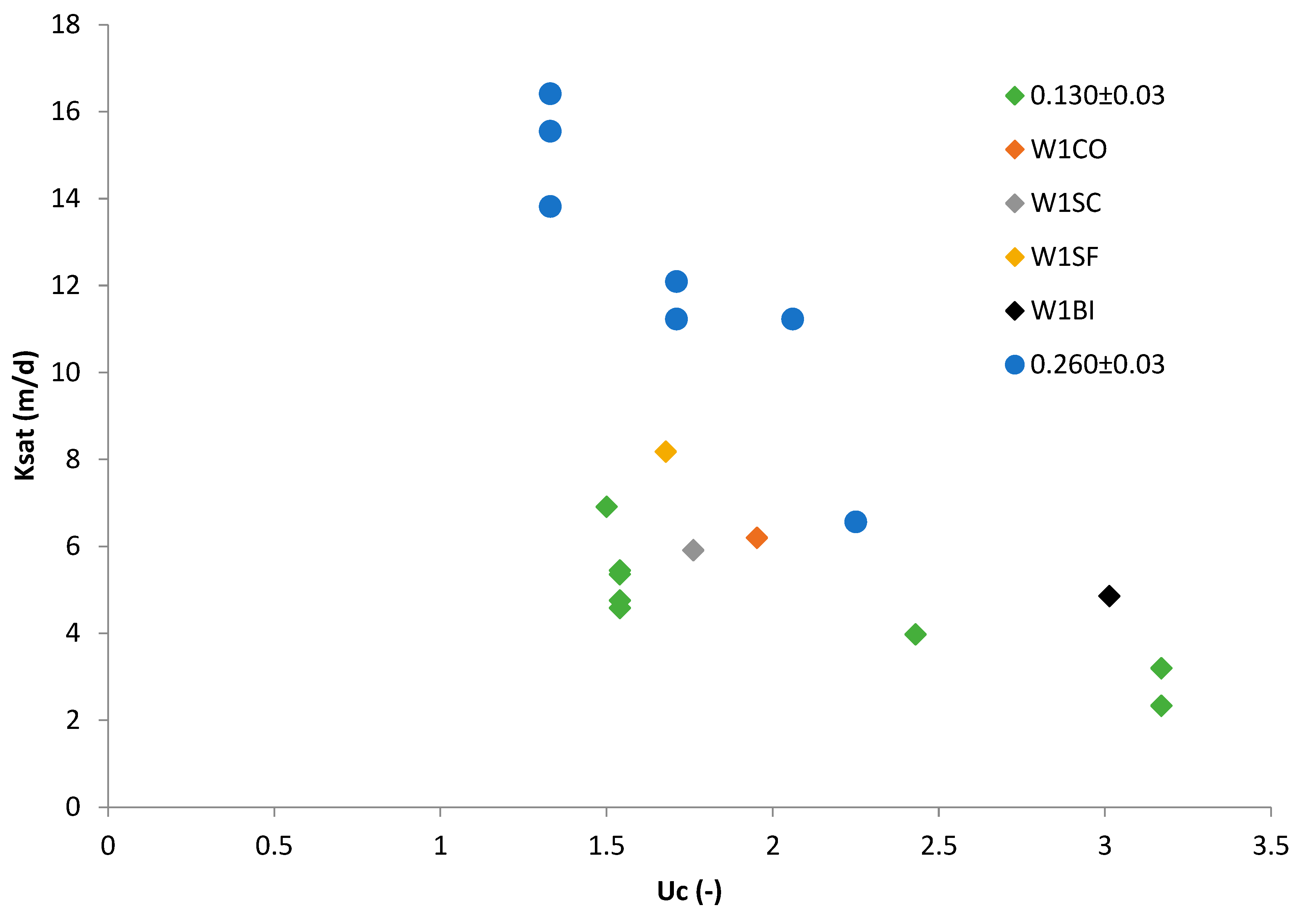
32], the saturated hydraulic conductivity decreases with decreasing uniformity, as shown in
Figure 5. This tendency is reflected by both existing experiments and our new experiments in the dataset of
Figure 5. Samples with a less uniform grain size distribution require higher gradients to initiate erosion as a result of lower saturated conductivity. Additionally, the influence of uniformity coeffect intensifies with a larger median grain size. Thus, a proper description of flow velocity as per Darcy’s law means that accurately describing saturated conductivity in terms of grain size distribution becomes paramount to determining the flow velocity required to initiate the initiation of backward erosion as indicated by Stokes’ law Equation (1).
Notably, the W1SF sample deviates from the general trend, and compared to the W1SC, the former has a higher saturated conductivity. This is despite W1SF being skewed towards the finer fraction, whereas a larger fine fraction usually results in a lower permeability [
33]. A possible cause for this is that this sample was not broad enough in order to be gap graded, leaving large pores through which the water could flow unimpeded as a result of imperfect sphere stacking, thus making it fall outside the expected trend.
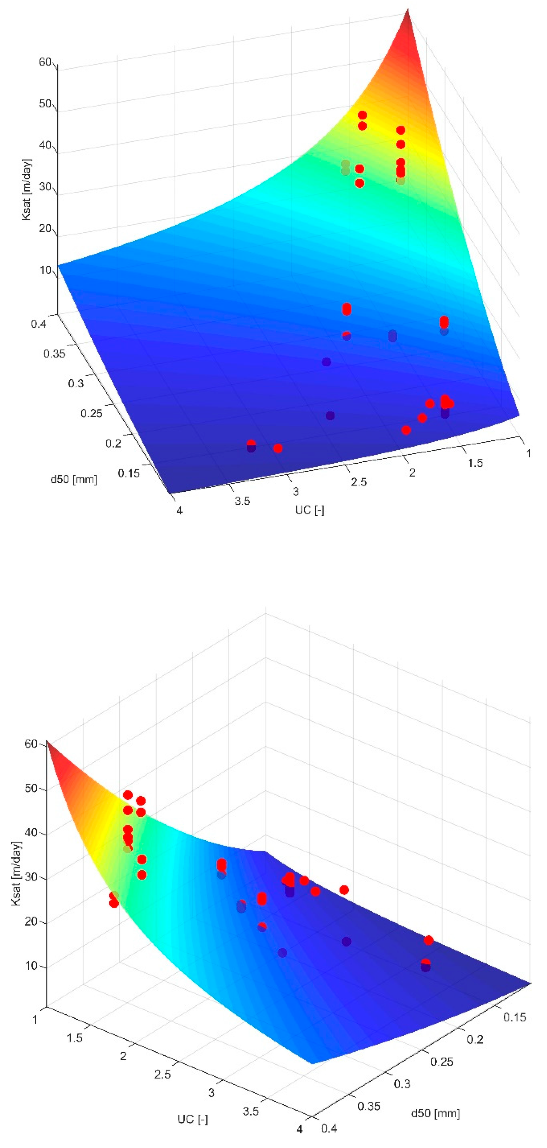
Figure 5 shows that the relationship between hydraulic conductivity and median grain size is also dependent on uniformity coefficient. When fitted on a log-log scale this relationship becomes linear, allowing for a fit on the following formula:
For this formula the variables a, b and c were fitted with a correlation coefficient of 0.956, the results of which are noted in
Table 3.
Using the values from
Table 3 the resulting formula was reworked to:
where
D50 is the median grain size in meters, returning saturated conductivity in meters per second. The resulting spread of this equation is shown in
Figure 6. Notable here is the increasing influence of
Uc on saturated conductivity with increasing median grain size and the increasing spread of the results.
4. Discussion
Although a clear relationship was established between the uniformity coefficient and median grain size and saturated conductivity, notable outliers from the trend derived from the database exist in the experiments. None of these samples in question was packed significantly differently (See
Table 1). In addition, the relationship Equation (3) was only determined for fine to medium sized sand mixtures. It would be advisable to test similar grain size distributions, but with different median grain sizes to determine if this trend persists towards the broader fraction.
Using Stokes’ law to relate the upward flow velocity provided an adequate fit for the range observed in the database, from 107 µm to 380 µm, with notably two outliers at 325 µm against the expected trend. Most notably, these have a higher saturated conductivity compared to similar experiments on the same sand, whereas they also stand out due to a lower relative density. Since this method only accounts for fluidisation at the top of the sample in the outflow point, this difference in relative density might be an indication of a lack of packing, locally increasing absolute flow velocities.
It is difficult to discern if this, or a different process becomes dominant when the sample approaches the diameter defining the lower boundary of very coarse sand to coarse sand (D50 > 0.42 mm), as outliers in that range show a lower flow velocity required to initiate erosion than as indicated by Stokes’ law (
Figure 4). This might be due to other effects, such as the finer fraction being washed out the porous medium at the onset of erosion, locally increasing permeability. The mechanism that underlies this deviation from the trend at that grain size diameter currently has no definitive explanation and will require more tests at larger median grain sizes. Deviations to the other side of the curve, those requiring higher flow velocities, can be explained by a lower saturated conductivity that is not encapsulated by just the uniformity coefficient and median grain size, such as the effects of vertical layering in the sample.
In addition, the equations used for both saturated conductivity and the moment of initiation require the bulk size of the sample to be large enough to filter out local incongruities, whereas the laboratory experiment had a small volume, exacerbating the influence of such incongruities if they are present. Tests on larger scale experiments will be required in order determine if such incongruities might have influenced the results and assess the exact precision of the results. If possible, this might resolve why the fine skewed sample was an outlier concerning its saturated conductivity [
32]. Beyond the expected spread in measured results these factors might also partially contribute to the range of the confidence interval in
Table 3. As there is a linear relationship between saturated conductivity and discharge, this confidence interval is expected to transfer linearly to the results calculated by Stokes Law.
Additionally, in its current configuration the experiment box funnels all water that enters the experiment to a single exit point. This results in the size of the box being a limiting factor for outflow velocity in terms of volume, i.e., the box is not large enough to contain significant areas of stagnant water. This limits the well capture area of the outflow point through the experiment dimensions. Although a few larger scale experiments are included in the database, they are too small in number to draw any meaningful discussions. More experiments to determine if the grain size distribution in relation to hydraulic gradient required for initiation in the established relationship has any effect beyond scaling with size could be beneficial [
33].
Although applicable in a laboratory setting, these results seem to hold up under less controlled circumstances, as a recent study [
34] was able to use Stoke’s equation somewhat successfully in reconstructing vertical transport from field conditions for four cases. These were, however, determined when piping was already in progress and vertical transport was most likely no longer the only limiting factor. More measurements at field conditions would be necessary in order to further explore the applicability of this theory in the field.
5. Conclusions
A good agreement was shown between Stokes’ law for vertical fluid flow and the initiation of transport of particles. It was also shown that considering the relation between hydraulic gradient, flow velocity (as used in Stokes’ law), and saturated conductivity, it is important to accurately assess saturated conductivity, in terms of grain size distribution. This allows for an assessment of the drag forces as a function of flow velocity experienced by the sand particles in the outflow point.
These results indicate that, in order to determine the gradient required to initiate backward erosion outside of these experiments, a description of saturated conductivity is required. Thus, following previous research [
35,
36], an estimate for bulk saturated conductivity in the experiment box was derived as a function of median grain size and uniformity coefficient. With an accurate estimate of bulk saturated conductivity, it should be possible to calculate the flow field and associated flow velocities near the outflow point. Tying this method in with Stokes’ law, this can be used as a predictor for the initiation of backward erosion, assuming the surface area of the exit point is known or can be predicted.
In terms of levee embankment design and maintenance this research can be of significance to determine accurately whether piping can occur given the subsurface conditions at a representative elementary volume. Whereas a bursting risk might exist due to hydraulic fracturing, or local disruptions of the cover layer could induce concentrated outflow, associated discharges might not be sufficient to induce piping. By using either a characteristic sand boil surface area or by measuring the potential breach beforehand, a determination can be made whether a sand boil will have the capacity to remove sand from the subsurface in the first place in terms of magnitude of flow velocity. This kind of knowledge is indispensable when assessing the safety of existing river embankments or when designing new flood protections, and can be used as a boundary condition in modelling piping risk for specific structures.
Assuming that an accurate description of the subsurface is available, the next challenge is to upscale our method from the experiment scale to the field scale for practical application. To this end, not only more laboratory experiments are required to accurately define the saturated conductivity from the samples, but also more field measurements, designed for adding to this line of research.
Author Contributions
W.-J.D. collected data, performed the experiments and wrote the manuscript with support from R.v.B. In addition Rens R.v.B. analytical methods. M.B. supervised the project. All authors provided critical feedback and helped shape the research, analysis and the manuscript. All authors have read and agreed to the published version of the manuscript.
Funding
This research was funded by Nederlandse Organisatie voor Wetenschappelijk Onderzoek (NWO), grant name: Piping in practice.
Acknowledgments
The Piping in Practice project is an NWO grant, funded by Arcadis Nederland, Deltares, Lievense, POV-Piping, Rijkswaterstaat, Stichting Toegepast Onderzoek Waterbeheer, Waterschap Rivierenland, Waterschap Drents Overijsselse Delta. The experiments in this paper were performed at the Deltares laboratory in Delft. Thanks go out to Vera van Beek for earlier comments on this paper.
Conflicts of Interest
The authors declare no conflict of interest. The funders had no role in the design of the study; in the collection, analyses, or interpretation of data; in the writing of the manuscript, or in the decision to publish the results.
Appendix A
Table A1.
Data on hole type piping experiments as reported in Van Beek, 2015a and Van Beek 2015. Experiment dimensions of some of these tests differ from the experiment used in this study. L is the distance to the exit hole from the inlet, Ls is the inside length, D, the thickness and W the width of the experiment container. D is the thickness of the acrylic plate. Dh is the diameter of the outflow point and d is the thickness of the acrylic plate. RD is the relative density, n is the porosity.
| Test No. | Reference | Sand Type | L (m) | Ls (m) | D (m) | W (m) | | Dh (mm) | d (mm) | RD | n | UC (–) | Ksat (m/s) | Hc/L(–) |
|---|
| B118 | [21] | Baskarp 1 | 0.344 | 0.48 | 0.1 | 0.3 | | 6 | 10 | 0.89 | 0.38 | 1.54 | 6.30 × 10⁻⁵ | 0.233 |
| W130 | [21] | Hoherstall Waalre | 0.344 | 0.48 | 0.1 | 0.3 | | 6 | 10 | 0.65 | 0.38 | 1.58 | 5.10 × 10⁻⁴ | 0.308 |
| W131 | [21] | Hoherstall Waalre | 0.344 | 0.48 | 0.1 | 0.3 | | 6 | 10 | 0.65 | 0.38 | 1.58 | 5.40 × 10⁻⁴ | 0.25 |
| B132 | [21] | Baskarp 1 | 0.344 | 0.48 | 0.1 | 0.3 | | 6 | 10 | 0.65 | 0.38 | 1.54 | 9.30 × 10⁻⁵ | 0.189 |
| B133 | [21] | Baskarp 1 | 0.344 | 0.48 | 0.1 | 0.3 | | 6 | 10 | 0.65 | 0.38 | 1.54 | 9.50 × 10⁻⁵ | 0.189 |
| B142 | [21] | Baskarp 1 | 0.344 | 0.48 | 0.1 | 0.3 | | 6 | 10 | 0.91 | 0.35 | 1.54 | 6.20 × 10⁻⁵ | 0.233 |
| B143 | [21] | Baskarp 1 | 0.344 | 0.48 | 0.1 | 0.3 | | 12 | 10 | 0.91 | 0.35 | 1.54 | 5.50 × 10⁻⁵ | 0.244 |
| B144 | [21] | Baskarp 1 | 0.344 | 0.48 | 0.1 | 0.3 | | 12 | 10 | 0.91 | 0.35 | 1.54 | 5.30 × 10⁻⁵ | 0.247 |
| B145 | [21] | Baskarp 1 | 0.344 | 0.48 | 0.1 | 0.3 | | 12 | 10 | 0.65 | 0.38 | 1.54 | 8.00 × 10⁻⁵ | 0.201 |
| B146 | [21] | Baskarp 1 | 0.344 | 0.48 | 0.1 | 0.3 | | 12 | 10 | 0.65 | 0.38 | 1.54 | 8.00 × 10⁻⁵ | 0.203 |
| I164 | [21] | Itterbeck 125-250 | 0.344 | 0.48 | 0.1 | 0.3 | | 6 | 10 | 0.97 | 0.34 | 1.71 | 1.30 × 10⁻⁴ | 0.328 |
| I165 | [21] | Itterbeck 125-250 | 0.344 | 0.48 | 0.1 | 0.3 | | 6 | 10 | 0.93 | 0.35 | 1.71 | 1.40 × 10⁻⁴ | 0.279 |
| I166 | [21] | Itterbeck mixture 1 | 0.344 | 0.48 | 0.1 | 0.3 | | 6 | 10 | 1 | 0.33 | 2.43 | 4.60 × 10⁻⁵ | 0.61 |
| I167 | [21] | Itterbeck mixture 2 | 0.344 | 0.48 | 0.1 | 0.3 | | 6 | 10 | 0.93 | 0.32 | 3.17 | 3.70 × 10⁻⁵ | 0.442 |
| I168 | [21] | Itterbeck mixture 2 | 0.344 | 0.48 | 0.1 | 0.3 | | 6 | 10 | 0.89 | 0.33 | 3.17 | 2.70 × 10⁻⁵ | 0.596 |
| E169 | [21] | Enschede sand | 0.344 | 0.48 | 0.1 | 0.3 | | 6 | 10 | 0.94 | 0.32 | 1.6 | 3.20 × 10⁻⁴ | 0.262 |
| S170 | [21] | Sterksel | 0.344 | 0.48 | 0.1 | 0.3 | | 6 | 10 | 0.89 | 0.37 | 2.25 | 7.60 × 10⁻⁵ | 1.017 |
| B171 | [21] | Baskarp 1 | 0.344 | 0.48 | 0.1 | 0.3 | | 6 | 10 | 0.9 | 0.35 | 1.54 | 6.80 × 10⁻⁵ | 0.23 |
| E172 | [21] | Enschede sand | 0.344 | 0.48 | 0.1 | 0.3 | | 6 | 10 | 0.94 | 0.33 | 1.6 | 3.40 × 10⁻⁴ | 0.247 |
| O140 | [21] | Oostelijke rivierenzand | 0.344 | 0.48 | 0.1 | 0.3 | | 6 | 10 | 0.65 | 0.35 | 2.06 | 2.00 × 10⁻⁴ | 0.276 |
| O141 | [21] | Oostelijke rivierenzand | 0.344 | 0.48 | 0.1 | 0.3 | | 6 | 10 | 0.65 | 0.35 | 2.06 | 2.10 × 10⁻⁴ | 0.262 |
| O163 | [21] | Oostelijke rivierenzand | 0.344 | 0.48 | 0.1 | 0.3 | | 6 | 10 | 0.94 | | 2.06 | 1.30 × 10⁻⁴ | 0.538 |
| 21 | [37] | Sand A | 0.7 | 0.96 | 0.2 | 0.2 | | 6 | 240 | 1 | | 1.3 | 4.00 × 10⁻⁴ | 0.18 |
| 22 | [37] | Sand A | 0.7 | 0.96 | 0.2 | 0.2 | | 6 | 240 | 1 | | 1.3 | 4.00 × 10⁻⁴ | 0.183 |
| 23 | [37] | Sand A | 0.7 | 0.96 | 0.2 | 0.2 | | 6 | 240 | 1.02 | | 1.3 | 3.90 × 10⁻⁴ | 0.181 |
| 24 | [37] | Sand A | 0.7 | 0.96 | 0.2 | 0.2 | | 6 | 240 | 1.05 | | 1.3 | 3.70 × 10⁻⁴ | 0.181 |
| 25 | [37] | Sand A | 0.7 | 0.96 | 0.2 | 0.2 | | 6 | 240 | 1 | | 1.3 | 4.00 × 10⁻⁴ | 0.18 |
| 26a | [37] | Sand A | 0.7 | 0.96 | 0.2 | 0.2 | | 6 | 240 | 0.976 | | 1.3 | 4.20 × 10⁻⁴ | 0.153 |
| 71 | [37] | Sand A | 2.6 | 3.52 | 0.3 | 0.6 | | 6 | 330 | 0.87 | | 1.3 | 4.70 × 10⁻⁴ | 0.106 |
| 73 | [37] | Sand A | 2.6 | 3.52 | 0.3 | 0.6 | | 6 | 330 | 0.8 | | 1.3 | 5.10 × 10⁻⁴ | 0.106 |
| 220883-4-1 | [38] | Beach sand | 2.4 | 5.75 | 1.5 | 0.5 | | 40 | 120 | 0.74 | | 1.33 | 1.80 × 10⁻⁴ | 0.196 |
| 220883-4-2 | [38] | Beach sand | 2.4 | 5.75 | 1.5 | 0.5 | | 100 | 120 | 0.74 | | 1.33 | 1.90 × 10⁻⁴ | 0.19 |
| 220883-4-3 | [38] | Beach sand | 4.5 | 5.75 | 1.5 | 0.5 | | 40 | 120 | 0.74 | | 1.33 | 1.80 × 10⁻⁴ | 0.192 |
| 220883-4-4 | [38] | Beach sand | 4.5 | 5.75 | 1.5 | 0.5 | | 100 | 120 | 0.74 | | 1.33 | 1.60 × 10⁻⁴ | 0.173 |
| Ims18 | [21] | Itterbeck 0.33 mm | 1.3 | 1.91 | 0.4 | 0.8 | | 20.5 | 20 | 0.87 | 0.35 | 1.6 | 3.50 × 10⁻⁴ | 0.254 |
| Bms1 | [21] | Baskarp 2 | 1.3 | 1.91 | 0.4 | 0.8 | | 20.5 | 20 | 0.94 | 0.37 | 1.5 | 8.00 × 10⁻⁵ | 0.162 |
| Ims20 | [21] | Itterbeck 0.33 mm | 1.3 | 1.91 | 0.4 | 0.8 | | 20.5 | 20 | 0.91 | 0.34 | 1.6 | 3.90 × 10⁻⁴ | 0.149 |
Table A2.
Properties of the sands used. D50 and D70 are the diameters of the 50 and 70 percent weight fractions respectively. Uc is the uniformity coefficient and nmin and nmax are the minimum and maximum wet porosities respectively.
Table A2.
Properties of the sands used. D50 and D70 are the diameters of the 50 and 70 percent weight fractions respectively. Uc is the uniformity coefficient and nmin and nmax are the minimum and maximum wet porosities respectively.
| Sand Type | D70 (μm) | D50 (μm) | Uc | nmin | nmax |
|---|
| Baskarp 1 | 154 | 132 | 1.54 | 0.34 | 0.469 |
| Baskarp 2 | 152 | 132 | 1.5 | 0.367 | 0.477 |
| Enschede sand | 431 | 380 | 1.6 | 0.32 | 0.411 |
| Hoherstall Waalre | 400 | 341 | 1.58 | 0.35 | 0.45 |
| Oostelijke rivierenzand | 307 | 233 | 2.06 | 0.322 | 0.423 |
| Itterbeck 0.33 mm | 410 | 342 | 1.6 | 0.337 | 0.434 |
| Itterbeck 125-250 | 278 | 219 | 1.71 | 0.345 | 0.465 |
| Itterbeck mixture 1 | 223 | 162 | 2.43 | 0.333 | 0.45 |
| Itterbeck mixture 2 | 203 | 143 | 3.17 | 0.319 | 0.44 |
| Sand A | | 325 | 1.28 | 0.41 | 0.51 |
| Sterksel | 300 | 228 | 2.25 | 0.357 | 0.474 |
References
- Kurdistani, S.M.; Tomasicchio, G.R.; D’Alessandro, F.; Hassanabadi, L. River bank protection from ship-induced waves and river flow. Water Sci. Eng. 2019, 12, 129–135. [Google Scholar] [CrossRef]
- Richards, K.S.; Reddy, K.R. Critical appraisal of piping phenomena in earth dams. Bull. Int. Assoc. Eng. Geol. 2007, 66, 381–402. [Google Scholar] [CrossRef]
- Vrijling, J.K. Piping: Realiteit of rekenfout? ENW Rapport; Rijkswaterstaat, Waterdienst: Brussels, Belgium, 2010; pp. 3–23. [Google Scholar]
- Förster, U.; Van den Ham, G.; Calle, E.; Kruse, G. Zandmeevoerende Wellen. Deltares Rapport Voor Rijkswaterstaat; 1202123-003-GEO-0002; Waterdienst: Offenbach, Germany, 2012. [Google Scholar]
- Veiligheid van Nederland in Kaart; Document HB 2540621; Rijkswaterstaat Projectbureau VNK: Den Haag, The Netherlands, 2015; pp. 120p.
- Dezert, T.; Fargier, Y.; Lopes, S.P.; Côte, P. Geophysical and geotechnical methods for fluvial levee investigation: A review. Eng. Geol. 2019, 260, 105206. [Google Scholar] [CrossRef]
- Glynn, M.E.; Quinn, M.C.; Kuszmaul, J. Predicting Piping Potential Along Middle Mississippi River Levees; Société Hydrotechnique de France: Paris, France, 2012. [Google Scholar]
- Van Beek, V.M.; Knoeff, H.; Sellmeijer, H. Observations on the process of backward erosion piping in small-, medium- and full-scale experiments. Eur. J. Environ. Civ. Eng. 2011, 15, 1115–1137. [Google Scholar] [CrossRef]
- Rijkswaterstaat. Schematiseringshandleiding Piping 2017; Ministerie van Infrastructuur en Milieu: Den Haag, The Netherlands, 2017. [Google Scholar]
- Stouthamer, E.; Berendsen, H.J. Factors Controlling the Holocene Avulsion History of the Rhine-Meuse Delta (The Netherlands). J. Sediment. Res. 2000, 70, 1051–1064. [Google Scholar] [CrossRef]
- Mol, J. Complex confining layers. Architecture and hydraulic properties of holocene and late weichselian deposits in the Fluvial Rhine-Meuse delta, The Netherlands. Sediment. Geol. 1997, 114, 322–323. [Google Scholar] [CrossRef]
- Bierkens, M.F.; Weerts, H.J. Block hydraulic conductivity of cross-bedded fluvial sediments. Water Resour. Res. 1994, 30, 2665–2678. [Google Scholar] [CrossRef]
- Bierkens, M.F. Complex Confining Layers: A Stochastic Analysis of Hydraulic Properties at Various Scales; Koninklijk Nederlands Aardrijkskundig Genootschap/Faculteit Ruimtelijke Wetenschappen, Universiteit Utrecht: Utrecht, The Netherlands, 1994. [Google Scholar]
- Kanning, W. The Weakest Link: Spatial Variability in the Piping Failure Mechanism of Dikes; TUDelft: Delft, The Netherlands, 2012. [Google Scholar]
- Sellmeijer, J.B. On the Mechanism of Piping under Impervious Structures; TUDelft: Delft, The Netherlands, 1988. [Google Scholar]
- Sellmeijer, H.; de la Cruz, J.L.; van Beek, V.M.; Knoeff, H. Fine-tuning of the backward erosion piping model through small-scale, medium-scale and IJkdijk experiments. Eur. J. Environ. Civil Eng. 2011, 15, 1139–1154. [Google Scholar] [CrossRef]
- Rozycki, A. Evaluation of the streaming potential effect of piping phenomena using a finite cylinder model. Eng. Geol. 2009, 104, 98–108. [Google Scholar] [CrossRef]
- Hijma, M.; Van der Meij, R.; Lam, K.S. Grasping the Heterogeneity of the Subsurface: Using Buildup Scenarios for Assessing Flood-Protection Safety. Geotech. Saf. Risk 2015, 924–929. [Google Scholar] [CrossRef]
- Polanco-Boulware, L.; Rice, J.D. Reliability-Based Three-Dimensional Assessment of Internal Erosion Potential due to Crevasse Splays. J. Geotech. Geoenviron. Eng. 2017, 143, 04016111. [Google Scholar] [CrossRef]
- Martínez, M.F.G.; Gottardi, G.; Marchi, M.; Tonni, L. On the Reactivation of Sand Boils Near the Po River Major Embankments. In National Conference of the Researchers of Geotechnical Engineering; Springer: Cham, Switzerland, 2019; pp. 328–337. [Google Scholar]
- Van Beek, V.M.; Van Essen, H.M.; VandenBoer, K.; Bezuijen, A. Developments in modelling of backward erosion piping. Géotechnique 2015, 65, 740–754. [Google Scholar] [CrossRef] [Green Version]
- Hoffmans, G.J.; Van Rijn, L. Hydraulic approach for predicting piping in dikes. J. Hydraul. Res. 2017, 56, 268–281. [Google Scholar] [CrossRef]
- Bligh, W.G. Submerged weirs founded on sand. In Dams and Weirs; American Technical Society: Chicago, IL, USA, 1915; pp. 151–179. [Google Scholar]
- Lane, E.W. Security from under-seepage masonry dams on earth foundations. Trans. Am. Soc. Civil Eng. 1935, 100, 929–966. [Google Scholar]
- Seed, H.B.; Duncan, J.M. The failure of Teton Dam. Eng. Geol. 1987, 24, 173–205. [Google Scholar] [CrossRef]
- Panda, M.N.; Lake, L.W. Estimation of Single-Phase Permeability from Parameters of Particle-Size Distribution. AAPG Bull. 1994, 78, 1028–1039. [Google Scholar] [CrossRef]
- Van Beek, V.; VandenBoer, K.; Bezuijen, A. Influence of sand type on pipe development in small- and medium-scale experiments. In Proceedings of the 7th International Conference on Scour and Erosion; CRC Press: Leiden, The Netherlands, 2014; Volume 1, pp. 111–120. [Google Scholar]
- Beard, D.C.; Weyl, P.K. Influence of Texture on Porosity and Permeability of Unconsolidated Sand. AAPG Bull. 1973, 57, 349–369. [Google Scholar] [CrossRef]
- Kutílek, M.; Nielsen, D.R. Soil hydrology: Texbook for Students of Soil Science, Agriculture, Forestry, Geoecology, Hydrology, Geomorphology and other Related Disciplines; Catena Verlag: Cremlingen-Destedt, Germany, 1994. [Google Scholar]
- Bierkens, M.F.P. Modeling Hydraulic Conductivity of a Complex Confining Layer at Various Spatial Scales. Water Resour. Res. 1996, 32, 2369–2382. [Google Scholar] [CrossRef]
- Stokes, G.G. Mathematical and Physical Papers; Cambridge University Press: Cambridge, UK, 1880; Volume 1. [Google Scholar]
- Odong, J. Evaluation of empirical formulae for determination of hydraulic conductivity based on grain-size analysis. J. Am. Sci. 2007, 3, 54–60. [Google Scholar]
- Severino, G.; De Bartolo, S. Stochastic analysis of steady seepage underneath a water retaining wall through heterogeneous stratified porous formations. J. Fluid Mech. 2015, 778, 253–272. [Google Scholar] [CrossRef]
- Fallico, C.; Ianchello, M.; De Bartolo, S.; Severino, G. Spatial dependence of the hydraulic conductivity in a well-type configuration at the mesoscale. Hydrol. Process. 2018, 32, 590–595. [Google Scholar] [CrossRef]
- Effing., B.; Taal, L. POV Piping-Wellen Onderzoek Monitoren en Karakteriseren van Wellen & Piping bij Waterkeringen. 2018. Available online: pov-piping.nl (accessed on 21 September 2020).
- Alyamani, M.S.; Sen, Z. Determination of Hydraulic Conductivity from Complete Grain-Size Distribution Curves. Ground Water 1993, 31, 551–555. [Google Scholar] [CrossRef]
- Hanses, U. Zur Mechanik der Entwicklung von Erosionskanälen in Geschichtetem Untergrund unter Stauanlagen. Ph.D. Thesis, Technischen Universität Berlin, Berlin, Germany, 1985. [Google Scholar]
- De Wit, J.M. Onderzoek zandmeevoerende wellen Rapportage Modelproeven. In Grondmechanica Delft Report CO-220887/10; Deltares (Geodelft): Delft, The Netherlands, 1984. [Google Scholar]
© 2020 by the authors. Licensee MDPI, Basel, Switzerland. This article is an open access article distributed under the terms and conditions of the Creative Commons Attribution (CC BY) license (http://creativecommons.org/licenses/by/4.0/).


