A Study on an Integrated Water Quantity and Water Quality Evaluation Method for the Implementation of Integrated Water Resource Management Policies in the Republic of Korea

Abstract

The existing methods of river evaluation tend to focus exclusively on water quantity; therefore, they do not provide a suitable methodology for integrated water management. In this study, research was carried out to develop an integrated river evaluation system that can simultaneously consider water quantity and water quality to improve the existing river evaluation methods. To this end, specific indicators were established to evaluate water quantity and water quality; moreover, an integrated evaluation formula was developed to express each indicator as an index. The integrated evaluation formula used additive functions and enabled integrated and comprehensive river evaluation through the sum of each indicator’s indices. The research subjects were rivers in the Paldang watershed, which surrounds important water resources in rep. of Korea. The rivers were analyzed using the study’s integrated river evaluation formula to identify the deteriorated grade of the water quality as well as the water quantity. Finally, the results of the integrated river evaluation rating were found to be poor or very poor. Based on this, the study determined that an integrated river management policy is required to simultaneously consider water quantity and water quality to restore the integrity of the rivers in the Special Countermeasures Area. The existing evaluations of rivers, which had been conducted only with a focus on water quantity, could be judged narrow or incomplete results. Based on this finding, it was also possible to identify an urgent need for a basic river management plan that can consider both water quantity and water quality organically. Ultimately, the study demonstrated that its methodology was able to make highly intuitive judgments about rivers’ current conditions; thus, it can be utilized to generate basic data for the establishment of customized river management policies.

1. Introduction

Globally, water and land resources are highly vulnerable and they exist within an organic relationship with significant mutual influence. To properly manage these vulnerable resources, adequate water availability, food supply, and sustainability of public health must be ensured [1]. In particular, water is an essential resource needed to sustain the life of animals and plants. Therefore, water management is extremely important. Countries around the world have established paradigms for water management policies in accordance with current needs as well as establishing and implementing water management policies. The need for Integrated Water Resource Management (IWRM) to ensure water quality became more urgent in the 1970s due to an increased interest in water quality. Rising interest in sustainable development in the 1980s and disasters caused by climate change, population growth, and water pollution in the 1990s further contributed to the urgent need to establish IWRM. IWRM began as a conceptual framework in the 1970s [2] and it has been expanded over time by its capacity to solve water problems and assist with complex decision-making [3]. IWRM became more important in the political arena by the early 1990s [4].

Inspired by the basin and ecosystem management approach, IWRM was reflected in the global summit agenda in the Dublin Principles on Water in 1992 and in Rio in 1992 [5,6], as global leaders recognized the need for a holistic approach to water management. The World Summit on Sustainable Development (WSSD) in 2002 featured IWRM as a key factor in achieving sustainable development. The Johannesburg Plan of Implementation (JPIO) was agreed upon with the support of developing countries, and the IWRM Guidelines at River Basin Level were announced at the 5th World Water Forum in 2009. In addition, in the Fourth World Water Development Report [7] (as in the Third Water Development Report), IWRM was still heavily discussed. Thus, many countries around the world continue to deepen their interest in IWRM.

Water management (such as IWRM) requires conservation and protection of resources to balance water use and population growth while maintaining those water resources’ functions and characteristics [8]. Korea’s water management strategies have led to development-oriented, unbalanced growth due to the process of rapid economic growth and development. In particular, the absence of a control tower at the central government of the Republic of Korea has made mutual coordination and cooperation between water-related ministries difficult. Conflict and competition have further exacerbated the problem. Therefore, factors related to water management should be integrated and managed in the basin unit. However, plans are implemented individually by ministries and facilities, leading to problems such as inefficiency, lack of fairness and sustainability, frequent flood damage, wasted budgets due to overlapping and over-investment, disputes over multipurpose dams and wide-area water supply, and conflicts over water distribution between regions.

Since the quality of human life is directly affected by the degree of conservation of water resources [9,10], the rep. of Korean people have continuously pointed out the problems of water resource management to the central government to improve their own quality of life and to secure stable water resources. The government has called for water management policies to ensure that all assets related to water resources, such as rivers in the watershed and areas around rivers, can become assets enabling people to live happily.

In response to Korean citizens’ demands, the Korean government enacted the Framework Act on Water Management in 2019 based on the IWRM concept. The government also launched the Integrated Water Management Committee in June of the same year to improve the water management system that had been divided based on water quantity and water quality until 2018. Additionally, the Korean government established a basic master plan for integrated management of both water quantity and water quality based on the integration of water-related national organizations.

The aforementioned water resource plan should be able to better understand the water resource system and provide comprehensive, accurate, and appropriate information on water availability across various times and space scales [11]. However, this national-level master plan for integrated water quantity and water quality management remains a somewhat vague concept for the Republic of Korea. The ambiguous standards of integrated water management have added to the confusion over water management policies. In particular, it is difficult to estimate even the most basic conditions of water resources in Korea because no evaluation system can simultaneously diagnose water quantity and water quality.

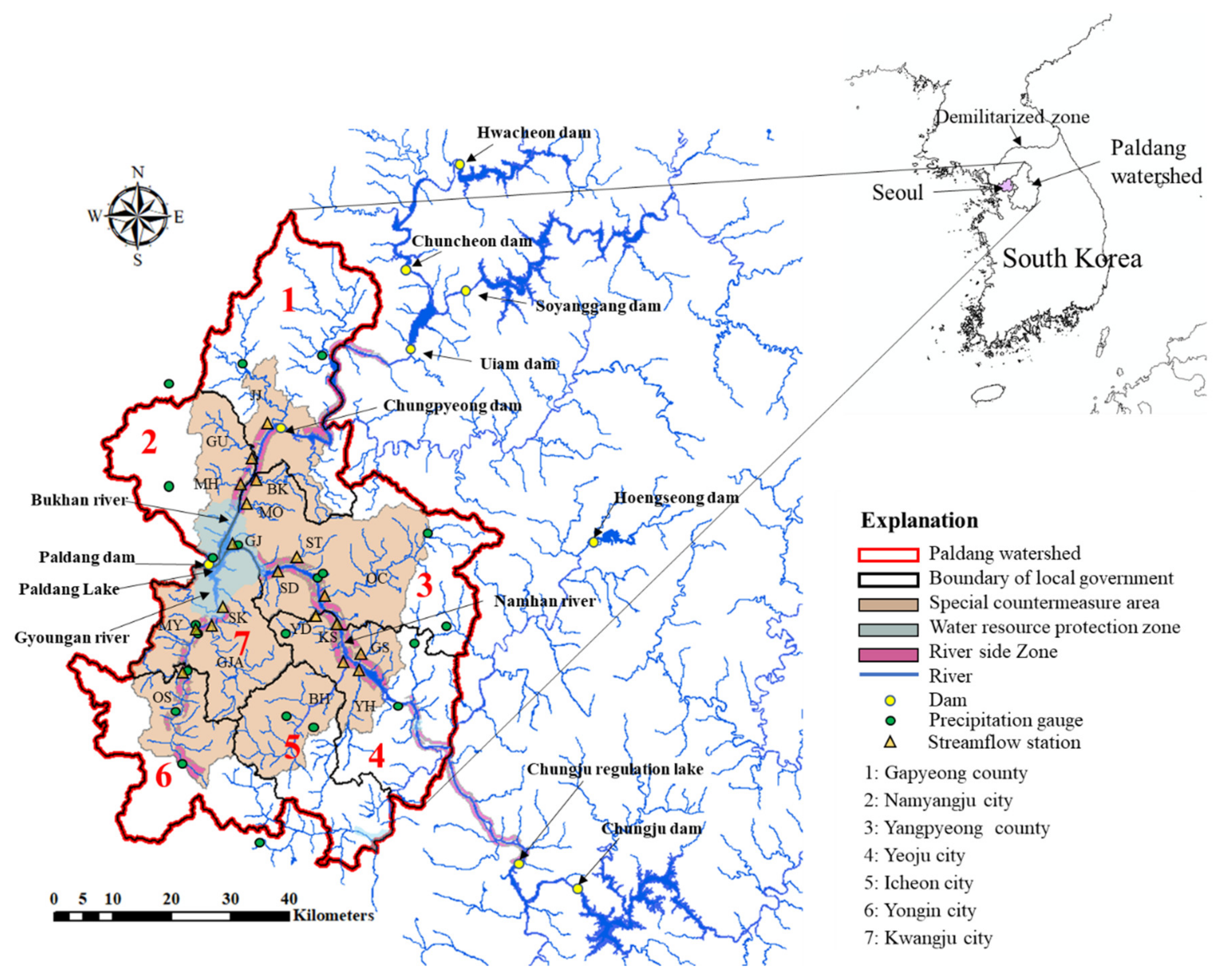
Therefore, the establishment of a detailed integrated watershed management plan for the Paldang watershed—which includes seven cities and counties surrounding Paldang Lake as well as Paldang Lake itself, adjacent to Seoul—is urgently needed. Paldang Lake presents a rare case as it is a water resource used by about 50 percent (approximately 25 million people) of the Republic of Korea’s population. Thus, Paldang Lake’s water management is one of the essential policy concerns for the central government. Thus far, the Korean government has set Paldang Lake’s water quality at 1.0 ppm based on BOD as a national goal to secure the lake’s stability. The government has also implemented very strict location regulations by establishing a water resource protection zone, a Special Countermeasure Area (SCA), and waterfront areas (such as riparian buffer zone) within the Paldang watershed that directly affect the lake. These overly strict protections and regulations to preserve Paldang Lake’s water quality have undermined the quality of life and welfare of local residents within the Paldang watershed. Moreover, these measures have suppressed the desire for strong development based on topographic characteristics. Public resistance to the central government is gradually increasing, played out in conflicts between local residents and the government regarding the SCA. Given that the government is no longer able to withstand public pressure regarding efficient water management, there is an urgent need to establish integrated water management measures for the Paldang watershed. Within this context, the development of an efficient evaluation system that can accurately diagnose current conditions should be the top priority. The technologies of water management of the EU and the USA in the field of IWRM are in the stabilization stage. In response to the era of a knowledge-based economy, the EU set up the European Research Area (ERA), centered on its member countries, and carried out the EU Framework Program, a core EU research and development project, five times since 1984 [12]. In the 1990s, Waterware, a decision-making system for river basin planning, was developed, and Water Framework Directive was established to improve water management across Europe drastically [13]. In the U.S., USBR developed Modular Modeling System [14], USGS and Tennessee Valley Authority developed RiverWare System [15], and EPA developed integrated modeling such as HSPF and SWAT to secure integrated water resource management technology through joint development and sharing of water quality and water quality management systems, as well as to collect water quality and water supply information at the national level. These models produce detailed results by sector in figures, but some areas are difficult to understand for policy-makers, decision-makers, or the general public, such as general administrators, not experts concerned.

Thus, specific tools for diagnosing, evaluating, and continuously monitor current conditions are needed to facilitate understanding of river conditions and provide directions for direct policymaking; indicators and indices can fulfill such a function. Annual investigation cases related to indicators and indices for water management have been reported in the Water Stress Index [16] (widely used worldwide), the Water Lack Index [17], the Water Poverty Index [18] (developed for sustainable water use), and the Climate Vulnerabilities Index [19] to assess the vulnerability of water-related floods and droughts. Additionally, reports have been published evaluating indicators around the world considering human water security and its interaction with river biodiversity [20]. Research has also been conducted in Korea on topics such as flood and drought management and securing water resources for water management.

However, most of the aforementioned prior studies have focused on water use and management, water distribution, vulnerability, and sustainability. All of these areas are biased towards water quantity, so they do not reflect an integrated water management paradigm that takes into account rivers’ characteristics, water quality, and ecology, among other factors. Therefore, this study intends to develop an integrated evaluation system for river water quality and water quantity using indicators and indexes that can be implemented in particular areas of conflict within the Paldang watershed. Moreover, the study’s findings can promote the smooth implementation of an integrated water management system and propose a useful methodology for similar watersheds and environments.

2. Materials

2.1. Research Area

Paldang Lake is an artificial lake created by the Paldang Dam, which is located approximately 27.32 kilometers away from Seoul, the Republic of Korea’s capital city. Paldang Lake has a basin area of 23,800 km², a total reservoir capacity of 2.44 million m³, an effective reservoir capacity of 18 million m³, and a stay period of 5.4 days. The lake is made up of three rivers: Namhan River, Bukhan River, and Gyeongan River. The Paldang watershed consists of five cities and two counties (Gapyeong county, Gwangju city, Namyangju city, Yangpyeong county, Yeoju city, Yongin city, and Icheon city) based on administrative district (Figure 1).

The Paldang watershed is subject to regulations through six individual laws and related enforcement ordinances, enforcement rules, and notices. Three strongly regulated areas—a water resource protection zone, waterfront areas, and an SCA—have been established to promote stable water protection. The water source protection zone is 151.72 km² and it includes Paldang Lake. All facilities (residential facilities, restaurants, lodging facilities, livestock facilities, general buildings, waste disposal facilities, etc.) were banned in this zone after the law was enacted. Residential facilities were allowed until the enactment of the Act of 1975. The waterfront area is 145.32 km² and it overlaps the water source protection zone and the regulated area. Waterfront areas are designated along the riverside of Paldang Lake’s incoming river; this differentiates them from water source protection zones as these waterfront areas are added buffer strip zones to reduce non-point pollution sources. The SCA is 2096.46 km², the largest of the three regulated areas. Unlike the previous two regulated areas, development is possible in the SCA only when there are effective measures against water pollution; however, this is only a surface interpretation of the law and it is almost impossible in practice (

Table 1. The general status for regulation regions of the Paldang watershed.

City/County	Population (Persons)	Water Resource Protection Area (km2)	Waterfront Zone (km2)	Special Countermeasure Area (km2)
Sum	950,111	151.72	145.32	2096.46
Namyangju city	120,310 (12.7) 1	42.38 (27.9) 1	8.09 (5.6)1	194.92 (9.3) 1
Yongin city	186,762 (19.7) 1	-	24.21 (16.7)1	207.34 (9.9) 1
Icheon city	167,706 (17.7) 1	-	-	233.02 (11.1) 1
Gwangju city	327,723 (34.5) 1	83.63 (55.1)1	9.61 (6.6)1	430.96 (20.6) 1
Yeoju city	24,849 (2.6) 1	-	44.19 (30.4)1	247.62 (11.8) 1
Gapyeong county	20,990 (2.2) 1	-	26.25 (18.1)1	190.89 (9.1) 1
Yangpyeong county	101,771 (10.7) 1	25.71 (16.9)1	32.97 (22.7)1	591.71 (28.2) 1

¹ Parentheses represent the ratio of the total value of the item.

). As mentioned earlier, this study focuses on Paldang Lake’s SCA, which must urgently arrange and implement countermeasures for efficient management of water quantity, water quality conservation, and revitalizing the regional economies. Three national rivers in the SCA—Namhan River, Bukhan River, and Gyeongan River—flow into Paldang Lake. For this research, these three national rivers were designated as research subjects. However, an evaluation system developed with only three rivers is too limited and makes it impossible to accurately diagnose the status of tributaries. Thus, this type of evaluation system cannot be used as a basis for improving river management by region or sub-catchment. If used at an actual site, this will further complicate river management through unreliable or inaccurate diagnostic results. Therefore, 18 tributaries that flow directly into Namhan River, Bukhan River, and Gyeongan River were selected as the study’s subjects (Figure 1). This enabled the development of an integrated evaluation of rivers’ water quantity and water quality by the river.

2.2. Data Collection

This study collected water quantity and water quality data. Water quantity data require unimpacted flow data and current flow data (observed data) for 18 rivers. The unimpacted flow means the water quantity in the absence of a controlled flow due to the storage and outlet by a dam, the intake and return, or the consumption by the land-use change, etc., that is, the water quantity in which the artificial water requirement is not present. The calculation of long-term unimpacted flow is an essential factor for the establishment of rational and efficient water use and water supply plans and is used as a basis for the permission of water use; the Soil Moisture Storage Tank Model (SMS-TANK) was employed to estimate the unimpacted flow under the natural conditions of the past, excluding artificial effects. The rep. of Korea builds the top legal plan, the long-term comprehensive plan for water resource [21], calculation of flood volume, and future water resource utilization plan every ten years, using the SMS-TANK model. Therefore, in this paper, it was judged that it is appropriate to simulate unimpacted flow using the SMS-TANK model following the rep. of Korea’s situation. The current flow data were collected from the stream flow stations (Figure 1), which are officially provided by the Korean government through the WAMIS (National Water Management Information System web site [22]. These data reflected a period of 10 years from 1 January 2009 to 31 December 2018.

Water quality data officially provided by the Korean government were used in this study as well. The Ministry of Environment of Korea provides water data measured every eight days in Korea’s major rivers through a website called the Water Environment Information System (WEIS) [23], which is meant for public use and the promotion of research. This study collected data regarding seven water quality items from WEIS: Biochemical Oxygen Demand (BOD), Chemical Oxygen Demand (COD), Total Nitrogen (T-P), Total Phosphorus (T-P), Dissolved Oxygen (DO), Suspended Solid (SS), and Total Organic Carbon (TOC). The collection period was the same as the data collection period of 10 years for SMS-TANK, calculated at the average annual value and reflected in this study.

3. Methodology

The study’s research methodology consisted of four steps. First, an evaluation indicator for each water quantity and water quality section was selected and the corresponding data for each indicator were established. For water quantity, this study used data estimated through SMS-TANK. For water quality, the data were gathered from WEIS [23], as mentioned earlier. Subsequently, a normality review was conducted to determine the suitability of the collected data. Standardization work was carried out to utilize the data in statistical analysis. Second, a factor analysis (FA) was performed to determine the suitability of sector-specific indicators for assessing the sector. Only indicators that were validated were selected and used in the integrated river evaluation system. Third, an integrated evaluation formula for water quantity and water quality—expressed as an index—was developed to derive each river’s integrated evaluation index. To prevent indicators from affecting each other, the indicators’ weighted value was estimated and reflected in the integration formula. Moreover, a principal component analysis (PCA) was performed and the entropy weighted method (EWM) was employed. In the final step, the objective and intuitive criteria for an integrated river assessment model were proposed, and the results of the integrated river-specific water quality assessment were derived (Figure 2). IBM’s SPSS Statistic 22 was utilized to perform a statistical analysis of normality reviews, data standardization, FA, PCA, and EWM.

3.1. Soil Moisture Storage Tank Model (SMS-TANK)

3.1.1. SMS-TANK Structure

The tank model for soil moisture with a low-flow structure used to simulate the unimpacted flow of the target river is similar to the structure of the standard four-stage tank model (Figure 3) [24]. However, the prior model is characterized by adding soil moisture with a low-flow structure to the first-stage tank to simulate the process of rainfall falling on the ground surface and filling the soil’s porosity. The outflow calculation process is similar to that of the standard four-stage tank model. Rainfall enters the first-stage tank, the amount of evaporation acid is reduced in the first-stage tank, and low-flowing water in each tank leaks out through the side drain or penetrates the lower tank. The water leaked through each tank’s runoff holes is aggregated into components and converted into flow rates flowing into the river. As with the standard four-stage tank model, the first-stage tank will simulate surface runoff, the second-stage tank will simulate intermediate runoff, and the third- and fourth-stage tanks will simulate base runoff (i.e., underground runoff). The first-stage tank’s soil moisture with a low-flow structure is outlined as follows.

• The impoundment amount, which is being impounded in the soil, consists of primary soil moisture storage X_P and secondary soil moisture storage X_S. Each maximum impoundment amount is S₁ and S₂.
• The impoundment amount of the first-stage tank X_A consists of X_P and the free water of the first- stage tank X_F, which represents added rainfall and decreased evaporation. If X_A is less than S₁, then X_A becomes X_P, and the free water value becomes ‘0’. When X_A is greater than S₁, X_P is saturated, and the remaining saturated amount becomes free water.

  In the case of X_P ≤ X_P, X_P = X_P, X_F = 0

  In the case of X_P > X_P, X_P = S₁, X_F = X_F − S₁
• If X_P is not saturated and free water exists in the lower tank, it is supplied by the amount of T₁ from the lower tank to the upper tank. T₁ can be written as follows:

  $$T_1=K_1\left(1-X_P/S_1\right)$$
• There is also an exchange of moisture between primary soil moisture storage and secondary soil moisture storage, which can be expressed as T₂. A positive T₂ indicates a shift from primary soil moisture storage to secondary soil moisture storage while a negative T₂ indicates the opposite.

  $$T_2=K_2\left(X_P/S_2-X_S/S_2\right)$$

3.1.2. Methodology and Evaluation Method of Parameters in the SMS-TANK Model

For the model to properly simulate an actual runoff phenomenon, a reasonable estimation of model parameters is essential. These parameters are unknown values that cannot be theoretically calculated; thus, they should be estimated as accurately as possible from the rainfall-leakage data of the base. In this study, there were a total of 12 required parameters. The parameters of the tank model estimated by using optimization techniques consist of ten, the coefficient of the five runoff holes and three penetration holes of each tank, and two parameters related to soil moisture low flow.

It is very difficult to utilize the parameter estimation method based on a trial and error approach; therefore, various optimization techniques are frequently used to perform parameter estimation. This study employed the Shuffled Complex Evolution-University of Arizona (SCE-UA) algorithm [24], one of the calibration modules of the National Weather Service River Forecasting System (NWSRFS) of the U.S. National Weather Service.

The SCE-UA algorithm was designed with four characteristics to identify an optimal solution [25]: the combination of definitive and probabilistic approaches, the structural evolution of complexes, competitive evolution, and complex shuffling. The SCE-UA algorithm initially generates samples and splits them into complexes throughout the entire parameter space where the solution value exists. Each complex evolves independently using the downhill simplex algorithm [26]. Evolved complexes are re-mixed, and new complexes are created. The process of evolution and shuffling is repeated until the convergence condition is satisfied.

In this study, three indicators were used to evaluate the results of parameter estimation. The evaluation indexes included the Nash–Sutcliffe Efficiency (NSE), Ratio of Volume (ROV), and R² (Coefficient of Measurement). NSE represents the relative magnitude of the error variance for the sample variances of the observed values. Therefore, a result of one would indicate that the simulated results and the actual measurements are perfectly aligned. Additionally, the greater convergence to zero, the worse the model’s performance is determined to be (Equation (1)). Using the concept of volume, ROV is a representation of the ratio between the simulated volume and the actual volume, which is interpreted to be the same as the actual value when the ROV value is 1 (Equation (2)).

$$\mathrm{NSE}=1-{\sum }_{\mathrm{i}=1}^{\mathrm{N}}{({\mathrm{q}}_{\mathrm{t}}^{\mathrm{obs}}-{\mathrm{q}}_{\mathrm{t}}^{\mathrm{sim}})}^2 / {\sum }_{\mathrm{i}=1}^{\mathrm{N}}{({\mathrm{q}}_{\mathrm{t}}^{\mathrm{obs}}-{\mathrm{q}}_{\mathrm{mean}}^{\mathrm{sim}})}^2$$

(1)

$$\mathrm{ROV}={\sum }_{\mathrm{i}=1}^{\mathrm{N}}{\mathrm{q}}_{\mathrm{t}}^{\mathrm{sim}} / {\sum }_{\mathrm{i}=1}^{\mathrm{N}}{\mathrm{q}}_{\mathrm{t}}^{\mathrm{obs}}$$

(2)

Here, ${\mathrm{q}}_{\mathrm{mean}}^{\mathrm{obs}}$ represents the mean value of the observed flow (current flow), ${\mathrm{q}}_{\mathrm{t}}^{\mathrm{obs}}$ represents the observed value, and $q_t^{sim}$ represents the predicted value.

3.2. Selection of Indicators by Sector and Data Construction

Indicators are information extracted to summarize changes in a particular research subject. Thus, indicators help to observe changes in complex phenomena within an understandable framework. At the same time, they can assist in making political choices to enact changes in a desirable direction. There are three main methods to construct indicators: the cause-effect chain framework, the theme framework, and the asset framework. The cause-effect chain framework includes Pressure-State-Response (PSR) and Driving force-State-Response (DSR). PSR are based on interrelationships between environment and economic activities and arise problems in terms of effectiveness if the causality between indicators is not identified clearly. DSR uses the Driving Force instead of pressure in PSR structures to indicate the cause of changes in environmental conditions. The DPSIR (Driving force-Pressure-State-Impact-Response) [27] structure is used to assess social and economic systems and natural systems by segmenting DSR into pressure and state [28]. The theme framework has the setting indicator method, which divides the phenomena to grasp into sub-sections according to policy goals by sectors. Among the theme framework, Water Poverty Index [13], Social Water Stress/Scarcity Index [29], and Environmental Sustainability Index [30] were developed to evaluate the water resource of use, management status, or sustainability. The asset framework has a structure that derives the national assets by calculating interactions between different types of assets, including financial capital, products, natural, human, social, and institutional assets. However, this method is still in the early stage because climate or biological diversity is challenging to convert into the asset.

To prevent errors in the policy decision-making process, the method mentioned above recommends selecting indicators that avoid selecting indicators that do not conform to the research purpose, over-set indicators, and using unreliable data. In this study, in consideration of the recommendations, sector-specific indicators were selected based on the following four considerations.

• Are the indicators selected to evaluate water quality and quantity possible to represent the evaluation items?
• Are the evaluation items quantifiable?
• Are the data of the evaluation items available to be measure regularly and provide convenient and sustainable?
• In the process of building data of the evaluation items, can the reliability of data secure with statistical processing?

3.2.1. Selection of Water Quantity Evaluation Index and Data Construction by Indicators

As suggested in the Index of River Conditions (ISC) [31] (see

Table 2. The hydrologic evaluation indicators.

Indicators	Reasons for Selection
High flow	Acting as a natural disturbance of the river system. Remove vegetation and organic matter and relocate sequential processes of river circulation
Low flow	Changing the low flow rate changes the availability of river habitats. It can be a factor that leads to the reduction possibility of the viability of a colony of animals and plants in the long-term.
Zero flow	The longer the duration between the drought season and the no-flow period, the more damage is done to the aquatic ecosystem.
Variability	This indicator can examine the diversity of changes in a river’s ecosystem according to the magnitude of the flow variability.
Seasonality	An important indicator for observing changes in rivers’ ecosystems due to seasonal changes (divided into a flood season and low-water season).
SDD (Stream Depletion Days)	Acting as a natural disturbance of the river system. Degree of restorability of the river’s original function.

), this study’s evaluation indicators for water quantity were selected to assess rivers’ flow status using the Hydrologic Index—consisting of High flow, Low flow, Zero flow, Variability, and Seasonality—and the index of River Depletion Days (SDD). However, these are conceptual indicators; thus, producing numerical data is essential to use them as quantitative indicators. To this end, the Flow Stress Ranking (FSR) method was employed.

FSR is a method used to assess river flow management and environmental flow rate that can minimize the environmental impact of optimal water distribution and future development plans required for the utilization of water resources and the management of rivers’ health. FSR is an indexed method that defines water stress by identifying the difference in flow rate changes between the current flow and unimpacted flow caused by the extraction amount and impoundment amount in the basin [32]. The current flow rate and unimpacted flow rate in this study were calculated using the river’s current flow rate data and the unimpacted flow rate data simulated by the tank model. “Current flow” refers to a river’s current water flow rate while “unimpacted flow” refers to the flow rate of a river that has caused artificial disturbances in that river’s current flow rate, combining the amount of required water and the amount of water movement in and out of the basin. If there is a large difference between the current flow rate and the unimpacted flow rate, then water stress in the basin is high. In contrast, if there is a small difference, then the water stress is low. The methods for calculating using FSR based on data by indicators in Table 2 are as follows.

FSR is a method used to assess river flow management and environmental flow rate that can minimize the environmental impact of optimal water distribution and future development plans required for the utilization of water resources and the management of rivers’ health. FSR is an indexed method that defines water stress by identifying the difference in flow rate changes between the current flow and unimpacted flow caused by the extraction amount and impoundment amount in the basin [32]. The current flow rate and unimpacted flow rate in this study were calculated using the river’s current flow rate data and the unimpacted flow rate data simulated by the tank model. “Current Flow” refers to a river’s current water flow rate while “Unimpacted Flow” refers to the flow rate of a river that has caused artificial disturbances in that river’s current flow rate, combining the amount of required water and the amount of water movement in and out of the basin. If there is a large difference between the current flow rate and the unimpacted flow rate, then water stress in the basin is high. In contrast, if there is a small difference, then the water stress is low. The methods for calculating using FSR based on data by indicators in Table 2 are as follows.

1.

High flow (HF(Q₁₀))

A high flow rate acts as a natural disturbance of the river system, eliminating vegetation and organic matter, and relocating the sequential process of river circulation [32]. The index in this study measures the degree of high flow rate using actual measurements (current flow) and simulated measurements (unimpacted flow). Flow size is measured by calculating the high flow index, which is similar to the one used to calculate the low-flow index. The index of high flow by day is calculated based on excess flow rates of 8.3%, as Equation (3) shows, and 16.7%, as Equation (4) shows. However, in this study, rather than setting an index based on a single value, two intervals were used to deal with the high flow range.

$$H{F}_{8.3}=1-2·\left|P_{ile}\left(Q{8.3}_u\right)-P_{ile}\left(Q{8.3}_c\right)\right|$$

(3)

Here, $H{F}_{8.3}$ means the standardized index of high flow rate based on excess flow rate 8.3%, $Q{8.3}_c$ is the excess flow rate of 8.3% of the actual measurement, $Q{8.3}_u$ is the excess flow rate of 8.3% of the simulated measurement, $P_{ile}\left(Q{8.3}_c\right)$ is the probability of excess flow rate of 8.3% of the actual measurement, and $P_{ile}\left(Q{8.3}_u\right)$ is the probability of excess flow rate of 8.3% of the simulated measurement.

The high flow rate index is calculated as the average of the number of modified changes on which the excess flow rate of 8.3% is based as well as the number of modified changes on which the excess flow rate of 16.7% is based [33].

$$HF\left(Q_{10}\right)=\frac{H{F}_{8.3}+H{F}_{16.7}}{2}$$

(4)

Here, $HF(Q_{10})$ means the standardized index of low-flow rate, $H{F}_{8.3}$ is the standardized index of low-flow rate based on an excess flow rate of 8.3%, and $H{F}_{16.7}$ is the standardized index of low-flow rate based on an excess flow rate of 16.7%.

2.

Low flow (LF(Q₉₀))

Changing the low-flow rate may change the availability of river habitats and thus reduce the long-term viability of flora and fauna clusters [32]. The index herein represents a measure of the change in low-flow rates based on actual measurements and simulated measurements. The index is calculated using two flow thresholds, given that the low-flow rate is occasionally over 90% of the daily flow rate, and the low-flow rate is used every month. Based on that flow rate, one case exceeded 91.7% for one year (or 11 out of 12 months), as Equation (5) shows. Another case exceeded 83.3% for one year (or 10 out of 12 months), as Equation (6) shows.

$$L{F}_{91.7}=1-2·\left|P_{ile}\left(Q{91.7}_u\right)-P_{ile}\left(Q{91.7}_c\right)\right|$$

(5)

Here, $L{F}_{91.7}$ means the index of low flow rate for excess flow rate of 91.7%, $Q{91.7}_c$ is the excess flow rate of 91.7% of the actual measurement, $Q{91.7}_u$ is the excess flow rate of 91.7% of the simulated measurement, $P_{ile}\left(Q{91.7}_u\right)$ is the probability of excess flow rate of 91.7% of the actual measurement, and $P_{ile}\left(Q{91.7}_c\right)$ is the probability of excess flow rate of 91.7% of the simulated measurement.

The low-flow rate index is calculated as the average of the number of modified changes on which the excess flow rate of 91.7% is based as well as the number of modified changes on which the excess flow rate of 83.3% is based.

$$LF\left(Q_{90}\right)=\frac{L{F}_{91.7}+L{F}_{83.3}}{2}$$

(6)

Here, $LF(Q_{90})$ is the standardized index of low-flow rate, $L{F}_{91.7 }$ is the standardized index of low-flow rate based on excess flow rate of 91.7%, and $L{F}_{83.3}$ means the standardized index of low-flow rate based on excess flow rate of 83.3%.

3.

Zero flow

The zero-flow rate is a natural feature of temporary rivers and small rivers. However, the longer the period between the drought season and the zero-flow rate period, the more damage is done to the aquatic ecosystem [32]. The proportion of the zero-flow rate index simply reflects the difference in the proportion of the zero-flow rate that occurs under simulated and actual measurement conditions. Based on FSR, the zero-flow rate is defined as a period of little flow exceeding 99.5%, as Equation (7) of that period shows.

$$PZ\left(Q_{99.5}\right)=1-2·\left|MAX\left(P{Z}_u;P{Z}_c\right)-MIN\left(P{Z}_u;P{Z}_c\right)\right|$$

(7)

Here, $PZ(Q_{99.5})$ means the index of zero-flow rate (flow rate exceeding 99.5%), $P{Z}_{u }$ is the ratio of zero-flow rate under simulated measurement conditions, (flow rate exceeding 99.5%), and $P{Z}_{c }$ is the ratio of zero-flow rate under actual measurement conditions, (flow rate exceeding 99.5%).

4.

Variability

This index is similar to the seasonal amplitude index in that it reflects the one-year flow rate variability. The main difference is that, for a variation index, all day-to-day variability is measured instead of measuring a simple difference in the minimum and maximum daily flow rates. This index compares the coefficient of variation between actual measurements and the daily flow rate of the simulated measurements, as Equation (8) shows.

$$CV=\frac{MIN\left(C{V}_u;C{V}_c\right)}{MAN\left(C{V}_u;C{V}_c\right)}$$

(8)

Here, $CV$ means the index of daily variability, $C{V}_{c }$ is the daily coefficient of variation of the actual measurements, and $C{V}_{u }$ is the daily coefficient of variation of the simulated measurements.

5.

Seasonality

The flood period and the low-water period are important indices for assessing how flood-inundated zones and river ecosystems react [32]. This index provides a measure of period changes in the maximum/minimum monthly flow rate for both the simulated and actual flow rate. The index indicates what percentage of the annual maximum and minimum of the actual and simulated flow rates is based on the frequency distribution, as Equation (9) shows.

$$SP= \frac{1}{200}·\{{{\displaystyle \sum }}_{i=1}[MIN\left(PH{C}_i;PH{U}_i\right)]+{{\displaystyle \sum }}_{i=1}\left[MIN\left(PL{C}_i;PL{U}_i\right)\right]\}$$

(9)

Here, $SP$ means the seasonality index, $PH{C}_{i }$ is the percentage of annual basis in ith with maximum annual flow rate from actual measurements, $PH{U}_{i }$ is the percentage of annual basis in ith with maximum annual flow rate simulated measurements, $PL{C}_{i }$ is the percentage of annual basis in ith with minimum annual flow rate from actual measurements, and $PL{U}_{i }$ is the percentage of annual basis in ith with minimum annual flow rate from actual measurements.

6.

Stream Depletion Days (SDD)

SDD reflects the daily flow rate at each monitoring station and the flow rate of reported river maintenance. This indicator evaluates a river’s soundness according to the number of SDD. The evaluation methods for this indicator are as follows.

• The selected rivers’ representative observation stations will be evaluated by grade, and the criteria presented in『A Study on the Evaluation and Improvement Measures of the Phenomenon of River Depletion』 [34] will be reflected.
• The standard flow rate of the representative observation stations will be selected as the mean droughty flow rate of the natural state to calculate the actual number of days of the occurrence of the river flow rate.
• The mean droughty flow rate of the natural state per river basin will be calculated as the ratio of the basin area by river based on the mean droughty flow rate per river calculated in the long-term comprehensive plan for water resources [35].

3.2.2. Selection and Evaluation Criteria for Water Quality Evaluation

The water quality sector indicator is used to maintain a sound water ecosystem and to preserve water quality suitable for water use purposes. Therefore, this study selected the water quality sector as an indicator based on the distinction between natural and artificial elements. Detailed reasons for selecting specific indicators by sector are outlined in

Table 3. Detailed reasons for selecting specific indicators by sector.

Indicators	Reasons for Selection
BOD	Physicochemical water pollution indicator; factors influencing organic pollution. Organic carbon, which is very important in the pollution of surface water, can be expressed through BOD. Organic carbon not only produces an unpleasant taste but also causes toxic chemical reactions that affect the medium and spread of waterborne diseases. It also causes oxygen deficiency in the aquatic ecosystem, threatening individual inhabitants of that ecosystem.
COD	Physicochemical water pollution indicator, factors influencing organic pollution.
T-N	Pollution factor of nutrient salts, factor of riverside nutrition.
T-P	Pollution factor of nutrient salts, factor of riverside nutrition.
DO	Indicator of the review of dissolved oxygen content in water.
SS	Representative of particulate solids in water; an indicator of pollution level review.
TOC	Indicator used to examine the total amount of dissolved organic carbon in water and to review unknowns and contained factors in COD and BOD tests.

.

Natural factors are defined as the characteristics of water distribution by region based on measured water quality at actual observation spots. BOD, T-P, T-N, DO, and SS were selected as representative indicators. Artificial factors are defined as rivers’ marginal capacity due to the increase in pollutants caused by urban expansion, reckless development, etc. This indicator is used to assess whether the target water quality standards set at the terminal spot of the representative mid-watershed announced by the Ministry of Environment have been achieved.

The Ministry of Environment of Korea evaluates the achievement rate of the target standards for the representative spots of the medium-scale area by region on an annual basis. One of the purposes of this study was to examine the average water quality of each selected river by calculating whether the Ministry of Environment achieved the target water quality for each mid-watershed.

Table 4. The target water quality standard by mid-watershed.

Large-Scale Region	Mid-Watershed	Goal Criteria
				Biosafety Level (BSL)
Han river	Bukhan River	Very good	Ⅰa	Very good∼Good
	Namhan River	Good	Ⅰb	Very good∼Good
	Gyeongan River	Ordinary	Ⅲ	Good∼Ordinary

presents the target water quality standards for each mid-watershed 4. The water quality assessment methods used herein are as follows.

• For each mid-watershed, conduct monthly water quality assessment based on the target water quality standards [35] set by the ministry of environment of the rep. of Korea.
• Every month, calculate the number of months where the target water quality was achieved (months achieved/12).

3.3. Reviewing and Standardizing the Suitability of Collected Data

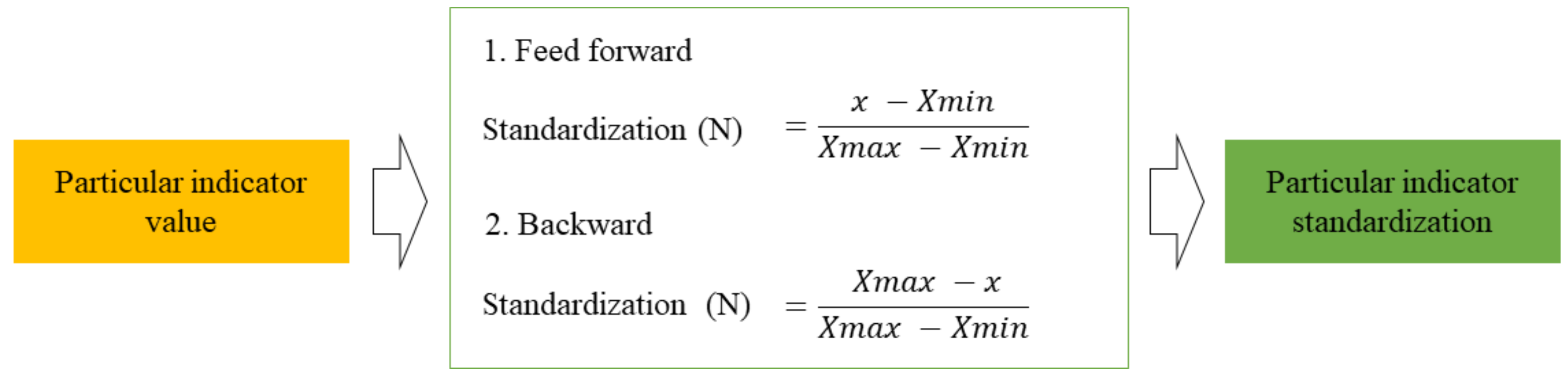
In processing the collected data, the data’s scope must be matched through normalization—or the data distribution should be transformed as needed—along with the data from different units to enable a comparative analysis of the statistical analysis results. It is essential to review raw data before performing statistical analysis using a frequency-based statistical methodology because the data are assumed to have a normal distribution. In this study, the normalization was conducted to determine the degree of bias and skewness of the data. A natural logarithm was used when the data’s skewness was greater than 1 and a common logarithm was used when the skewness was less than −1 to ensure normality.

Additionally, most collected raw data tend to be standardized before they are used for statistical analysis because they have different dimensions or scales. Thus, it is difficult to perform statistical analyses between data without standardization. Common standardization methods include Z-Score, rebalancing, category scale, baseline difference, mean upper and lower indicators, opinion balance, annual difference percentages, and circulation indicators [36]. As this study aims to develop a rating system through the calculation of an index, all indicators’ values should have unidirectional characteristics. However, some indicators may exhibit inverse relationships; therefore, a minimum-to-maximum standardization method was selected to standardize the data for statistical analysis (Figure 4).

3.4. Reviewing the Conformity of Indicators and Screening of Indicators

Based on the established data regarding water quantity and water quality, the validity and reliability of indicator selection for this study’s assessment were reviewed. FA was conducted for this purpose. Based on the analysis results, indicators suitable for integrated river health assessment were selected. Unreliable indicators and indicators that could not be interpreted by each factor were excluded. Before conducting FA, it is necessary to determine whether the data are suitable for such analysis. The suitability of the data is determined by using Kaiser–Meyer–Olkin’s (KMO) measure of sample conformity, Bartlett test, and communality. Generally, KMO values of >0.5 and the Bartlett test are considered appropriate for performing factor analyses with p < 0.1 and a communality of 0.5 or higher. Otherwise, the selection of variables for FA is considered to be poor [37,38,39,40]. In this study, the data’s suitability for FA was determined based on KMO adequacy, the Bartlett test, and communality prior to conducting said analysis.

Factors must then be extracted to perform FA. In this study, the PCA method was used to determine the number of factors. As an extraction method for determining the number of factors, only factors with an eigenvalue greater than 1 were extracted and analyzed. Factor rotation assumes that there is no correlation between factors; thus, the analysis was performed by selecting the varimax method out of possible orthogonal rotation methods.

3.5. Index Calculation and Weight Value Calculation Methods

3.5.1. Index Equation

An additive function can be used as a suitable methodology to evaluate integrated river health. The additive function is the simplest form of the summative function. In this study, indicators’ indices by sector can be proposed as the sum of the indices. However, if the individual sector indices are all combined, the aggregated indices may be overvalued, which can be counteracted by appropriately weighing each index per sector. The weighted general form of the additive integration function is equal to Equation (10), where the sum of the weights is given as 1.

$$I= {{\displaystyle \sum }}_{i=1}^n{W}_i·I_i$$

(10)

where ${{\displaystyle \sum }}_{i=1}^n{W}_i=1$, $I_i$ is the index of each indicator by sector and $W_i$ refers to the weight of each indicator by sector.

3.5.2. Weighted Value Calculation Methods

The weight required for Equation (10) should take into account the effect of the factors between the indicators. For this purpose, the PCA and entropy weighted methods (EWM) were implemented for each sector in this study. Additionally, the geometric mean method was applied as an aggregation method to prevent compensation problems caused by the offset effect (i.e., when the low indicator value is diluted by the high index value).

Subsequently, to equalize each indicator’s effect on the integrated index, the weighted value of the PCA and EWM with the least weight deviation for each indicator was selected as the weight to calculate the integrated index.

1.

Principal Component Analysis (PCA)

PCA is an analytical method that reduces the dimensions of several variables associated with each other and can generate a small number of new variables. It is critical to employ data processing techniques that can distinguish important variables, simplify calculations, and reduce dimensions for data visualization. To efficiently identify the correlations, present in the data, eigenvalue decomposition is applied to the components’ correlation matrix to obtain eigenvectors. Eigenvectors refer to the axes with the greatest correlation defined by the linear combination of components; i.e., a process of loading the principal component. Multiplying the data matrix by the eigenvector transforms the data of the main component axes and produces the PCA score. The equation for the first principal component can be defined as Equation (11) when the matrix of m × n data with m samples and n variable values is labeled X. The mean of each variable is 0 and the standard deviation is 1.

$$w_1=\begin{array}{c}\arg \max \left\{||,X_w||{}^2\right\}=\arg \max \left\{{\omega }^T{X}^T{X}_w\right\}\\ ||w||=1 ||w||=1 \end{array}$$

(11)

where argmax means a value of 1, $w$ in length that makes the function the maximum value.

2.

Entropy Weighted Method (EWM)

The EWM [41] is used to determine each property’s weight. In other words, this is a process of applying an information theory that is easy for decision-makers to understand so they can navigate complex decision-making issues with many alternatives. EWM is a method of weighting through the attribute information of the assessment items that are being used. This method is often employed to weight vulnerability assessments. The entropy method has the advantage of objectivity because it calculates weights by considering the distribution of secured data without relying on subjective judgment.

Four basic methods used to measure information based on entropy include maximum entropy, joint entropy, conditional entropy, and trans-information. Maximum entropy is derived from statistical physics research and it is a technique that excludes assumptions about unknown facts and sees only known partial facts as a source of knowledge acquisition. This technique can function as a probability model with a uniform distribution for other values if the predefined constraints are met. Maximum entropy is defined as the entropy amount of the probability $p(x_n)$ distribution of the discrete random variable $X=\left\{x_n\right\}$. Maximum entropy $H\left(X\right)$ refers to the uncertainty or information capacity of $X$, and limit entropy for hydrological random discrete variables is defined as Equation (12).

$$H\left(X\right)= -{{\displaystyle \sum }}_{n=1}^{N}p\left(x\right)·lnp\left(x\right)$$

(12)

Generally, if the discrete probability variable $X$ follows a uniform distribution, there is maximum entropy. Thus, having a uniform distribution of the maximum entropy model for unknown facts means that the model has maximum entropy for unknown content. This is considered to be the same probability for two events when there is no information to clearly distinguish a given event; in other words, this means that uncertainty is maximized, resulting in maximum entropy.

3.6. Evaluation Method of Rating by Index

This study intended to perform integrated river evaluation through the sum of the index values by sector. In general, the data range in a normal distribution is represented by the mean (μ) and the standard deviation (σ). When the standard deviation is 1σ in the normal distribution, the data range is 34.1% to the left and right, accounting for 68.27% of the total. When the standard deviation is 2σ, the data range is 47.7% to the left and right, accounting for 95.45% of the total.

In this study, the rating classification was based on the assumption that the calculated ‘index value’ was defined as variable X and that variable X followed a normal distribution; i.e., a Gaussian distribution. Standard deviation (1σ) 1 was classified into the highest and lowest grade sections, and 16% of the left and right classes were divided into the top 1 and bottom 5 classes, respectively. The remaining 68% were classified by selecting 0.5σ standard deviation as the classification criteria. Therefore, 84.0% to 100% of sections were evaluated by class 1 (μ + 1.0σ), 67.5% to 84.0% of sections as class 2 (μ + 0.5σ), 32.5% to 67.5% of sections as class 3 (μ ± 50.5σ), 16.0% to 32.5% of sections as class 4 (μ − 0.5σ), and the remaining sections as class 5 (μ − 1.0σ) (

Table 5. The rating section by the standard deviation.

Rating Section		Rating	Key Processing Function
μ + 1.0σ	100.0%∼84.0%	1	Very good (High)
μ + 0.5σ	84.0%∼67.5%	2	Good (Medium High)
-	67.5%∼32.5%	3	Acceptable (Medium)
μ − 0.5σ	32.5%∼16.0%	4	Poor (Medium Low)
μ − 1.0σ	16.0%∼0.0%	5	Very poor (Low)

).

4. Result and Discussion

4.1. Result of Data Construction

4.1.1. Water Quantity Data

To calculate water quantity (unimpacted flow) via the SMS-TANK model, the first step is to estimate the parameters. For this purpose, dam inflow data and river flow rate data located around the target rivers were used. Rainfall data were collected from the observations of 21 rain stations such as Figure 1 surrounding the target area, calculated using the Thiessen Method, and reflected in the model. There were 10 dams and 5 rivers, as

Table 6. The estimated spots’ parameters using the data on a total of 15 spots.

No.	Target	Basin Area (km2)	Remark	Abbreviation
1	Soyang	2703	Dam inflow rate	SY
2	Chungju	6648	Dam inflow rate	CJ
3	Chungju regulation area	1713	Dam inflow rate	CJC
4	Hoengseong	208	Dam inflow rate	HS
5	Guangdong	121	Dam inflow rate	KD
6	Goesan	677	Dam inflow rate	GS
7	Hwacheon	4085	Dam inflow rate	HC
8	Chuncheon	775	Dam inflow rate	CC
9	Uiam	281	Dam inflow rate	UA
10	Cheongpyeong	2268	Dam inflow rate	CP
11	Yeongwol 1	1524	River flow rate	YW1
12	Yeongwol 2	2283	River flow rate	YW2
13	Youngchun	4690	River flow rate	YC
14	Dalcheon	721	River flow rate	DC
15	Wontong	526	River flow rate	WT

shows. Data on these 15 total spots were used to estimate the spots’ parameters.

For parameter estimation, the initial low-flow height of the SMS-TANK was set to 240. The first-stage tank and the second-stage tank were set to 0, the third-stage tank was set to 10, and the fourth-stage tank was set to 500. The SCE-UA algorithm was employed [25]. As an analysis of the estimated parameters’ adequacy,

Table 7. Nash–Sutcliffe Efficiency (NSE) and Ratio of Volume (ROV) between the predicted and actual amounts for the same spots as in Table 6.

Target	Parameters of SMS-TANK												NSE	ROV
	A2	A1	A0	B1	B0	C1	C0	D1	HA2	HA1	HB	HC
SY	0.3959	0.1702	0.0838	0.0836	0.0502	0.0168	0.0283	0.0005	400	150	0.0	0.0	0.84	0.86
CJ	0.3793	0.0800	0.1225	0.0995	0.0503	0.0122	0.0179	0.0005	400	150	0.0	0.0	0.71	0.80
CJC	0.5000	0.3000	0.1580	0.0300	0.1000	0.0050	0.0500	0.0005	400	150	0.0	0.0	0.73	0.95
HS	0.4822	0.0960	0.0356	0.0743	0.0834	0.0051	0.0497	0.0005	400	150	0.0	0.0	0.90	1.09
KD	0.3173	0.1222	0.1104	0.0987	0.0369	0.0051	0.0492	0.0005	400	150	0.0	0.0	0.82	0.79
GS	0.5000	0.0974	0.2384	0.0784	0.0828	0.0050	0.0191	0.0005	400	150	0.0	0.0	0.80	0.82
HC	0.2783	0.0866	0.2031	0.0324	0.1000	0.0050	0.0500	0.0005	400	150	0.0	0.0	0.67	0.89
CC	0.4164	0.1808	0.1192	0.0890	0.0302	0.0050	0.0328	0.0005	400	150	0.0	0.0	0.80	0.78
UA	0.4979	0.2992	0.0947	0.0300	0.0999	0.0051	0.0479	0.0005	400	150	0.0	0.0	0.58	0.83
CP	0.5000	0.1972	0.0001	0.0416	0.0784	0.0050	0.0500	0.0005	400	150	0.0	0.0	0.59	0.91
YW1	0.5000	0.0300	0.1945	0.0811	0.0633	0.0062	0.0225	0.0005	400	150	0.0	0.0	0.62	0.85
YW2	0.2796	0.0300	0.1502	0.0964	0.1000	0.0107	0.0287	0.0005	400	150	0.0	0.0	0.40	0.76
YC	0.4312	0.0300	0.1386	0.0821	0.0408	0.0071	0.0050	0.0005	400	150	0.0	0.0	0.59	0.74
DC	0.4995	0.2283	0.2171	0.1000	0.0551	0.0054	0.0178	0.0005	400	150	0.0	0.0	0.55	0.92
WT	0.3910	0.0311	0.2997	0.0992	0.0830	0.0092	0.0471	0.0005	400	150	0.0	0.0	0.69	0.73

presents the NSE and ROV between predicted and actual amounts for the same spots as in Table 6. When determining a model’s quality via NSE, the threshold is set at 0.50 < NSE < 0.65. Then, models within this range are recommended [42]. If the value is 0.65 or higher, the model is judged to have excellent performance [43]. The NSEs for each spot in Table 7 were found to exceed 0; moreover, nine of these had values of 0.65 or higher. In addition, the ROV value was within the range of 0.73–1.09 and the minimum simulated amount was over 73% consistent with the actual amount. Thus, based on the NSE and ROV results, the estimated parameters were judged to be suitable for the amount simulation in this study.

The unimpacted flow data for the study’s 18 rivers in Figure 1 were estimated by reflecting the parameters derived earlier through SMS-TANK. Figure 5 shows changes in water quantity data by estimated spots. The largest simulated amount appeared in JJ in 2011 with 534.97 m³/day, while the smallest was predicted to be 0.02 m³/day in SD in 2009. Overall, the simulated unimpacted flow data pattern was mostly high in summer (between June and August) and low in winter (between November and February). The simulated unimpacted flow data were used as data for six water quantity indicators—High flow, Low flow, Zero flow, Variability, Seasonality, and SDD—employing the SDD evaluation criteria of Equations (1)–(7).

The largest simulated amount appeared in JJ in 2011 with 534.97 m³/day, while the smallest was predicted to be 0.02 m³/day in SD in 2009. Overall, the simulated amount pattern was mostly high in summer (between June and August) and low in winter (between November and February). The simulated amount data were used as data for six water quality indicators—High flow, Low flow, Zero flow, Variability, Seasonality, and SDD—employing the SDD evaluation criteria of Equations (1)–(7).

4.1.2. Water Quality Data

Water quality data were simulated by converting collected raw data into annual average data. Figure 6 illustrates the changes in water quality data of 18 rivers. Most rivers DOs are distributed on a 10.0 mg/L basis, and most BODs are found to be below 2.0 mg/L. Meanwhile, rivers such as GU, MH, and OS are above 2.0 mg/L. Most CODs range from 2.0 to 3.0 mg/L, but OS ranges from 5.0 to 6.0 mg/L, which is the highest value compared to other rivers. SS is at a higher level than other rivers, given that GS showed the highest value of 173.9 mg/L in 2015 but, after 2017, SS in all rivers was below 20.0 mg/L.

In the case of TN, MH was found to be in the range of 7.9 to 9.1 mg/L, higher than other rivers. The TN of other rivers was found to be emitted at an average level of 3.3 mg/L. TP was found to be below 0.06 mg/L in most rivers; however, in the case of GS, YH, and OS, the variation was shown to fluctuate significantly in the range below 0.38 mg/L. The TOC of OS showed the highest value compared to other rivers with an average of 6.0 mg/L, and the lowest TOC of OC with an average of 1.15 mg/L.

4.2. Determining the Data’s Suitability

A statistical analysis of the data was conducted to ensure that the data were normal and properly standardized. Any data showing skewed distribution were transformed through a logarithm to ensure maximum normality. A normality review was performed based on skewness, and the data were transformed by natural logarithm if the skewness value was 1 or higher or by common logarithm if it was −1 or lower.

Table 8. Variation in the skewness of water quantity data based on the normality review.

Classification	High Flow	Low Flow	Zero Flow	Variability	Seasonality	SDD
Before conversion	−2.526	−0.734	−2.998	−0.821	0.202	0.988
After conversion	1.216	−0.734	1.511	−0.821	0.202	−0.455

shows variations in the skewness of water quantity data based on the normality review, while

Table 9. Variation in the skewness of water quality data based on the normality review.

Classification	DO	BOD	COD	SS	T-N	T-P	TOC
Before conversion	−0.194	1.991	1.165	7.332	1.856	2.097	1.564
After conversion	−0.194	0.966	0.585	0.905	0.695	0.500	0.629

presents variations in the skewness of water quality data. Among the amount indicators, the skewness of Low Flow, Variability, Seasonality, and SDD were determined to have a normal distribution with values within the range of −1 and less than 1. High flow and Zero flow were found to be less than −1 and were determined to be non-normal; thus, the data were converted by common logarithm to ensure normality. Among the water quality indicators, only DO skewness was found to be within the range of −1 and 1 and therefore determined to have a normal distribution. All other indicators exhibited skewness greater than 1, which was judged to be a non-normal distribution. Thus, the data were converted by natural logarithm to ensure normality. In the subsequent process, all data were determined to be normally distributed, enabling standardization.

4.3. Conformity of Indicators and Results of Indicator Screening

KMO, the Bartlett test, and communality were assessed for all standardized data to determine whether the data were suitable for FA. The results showed that the KMO values of both water quantity and water quality were all above 0.5 and the Bartlett test results were all below 0.1, satisfying each criterion (see

Table 10. The results of Kaiser–Meyer–Olkin’s (KMO) values and Bartlett’s test by water quantity and water quality.

Contents		Water Quantity	Water Quality
KMO measure		0.617	0.839
Bartlett’s unit matrix test	Chi-squared approximation	221.636	1263.082
	p (probability)	<0.001	<0.001

). Additionally, communality values for all indicators of water quantity and water quality were 0.5 or higher (

Table 11. The results of the communality values by all indicators of water quantity and water quality.

Contents	Indicator	Extraction
Water quantity	High flow	0.830
	Low flow	0.734
	Zero flow	0.717
	Variability	0.744
	Seasonality	0.715
	SDD	0.732
Water quality	DO	0.998
	BOD	0.893
	COD	0.946
	SS	0.973
	T-N	0.846
	T-P	0.869
	TOC	0.893

). On that basis, all collected data intended to be used in this study were available for FA.

Table 12. The Varimax results for factor extraction.

Indicator		Initial Eigenvalue			Extraction Sum of Squares Load			Rotational Sum of Squares Load
		Total	Distributed%	Cumulative%	Total	Distributed%	Cumulative%	Total	Distributed%	Cumulative%
Water quantity	High flow	2.35	39.18	39.18	2.35	39.18	39.18	1.74	29.06	29.06
	Low flow	1.31	21.80	60.97	1.31	21.80	60.98	1.53	25.54	54.60
	Zero flow	0.81	13.56	74.54	-	-	-	-	-	-
	Variability	0.693	11.54	86.08	-	-	-	-	-	-
	Seasonality	0.52	8.66	94.74	-	-	-	-	-	-
	SDD	0.32	5.26	100.00	-	-	-	-	-	-
Water quality	DO	4.66	66.54	66.54	4.66	66.55	66.55	4.65	66.42	66.42
	BOD	1.05	14.96	81.50	1.05	14.96	81.51	1.06	15.09	81.51
	COD	0.74	10.50	92.00	-	-	-	-	-	-
	SS	0.24	3.44	95.45	-	-	-	-	-	-
	T-N	0.16	2.30	97.74	-	-	-	-	-	-
	T-P	0.11	1.52	99.26	-	-	-	-	-	-
	TOC	0.05	0.74	100.00	-	-	-	-	-	-

presents the varimax results for factor extraction. A review of the total variance of the water quantity sector showed that two main components, High flow and Low flow, accounted for 54.60% of the total. In the water quality sector, the two main components were DO and BOD, which accounted for 81.51% of the total.

The reference value of the rotated component matrix, which correlates with the indicators and the factor components, is ±0.4 or higher.

Table 13. The results of the rotated component matrix of water quantity and water quality.

Contents	Indicators	Components
		1	2
Water quantity	High flow	0.910	−0.002
	Low flow	0.069	0.676
	Zero flow	0.204	0.764
	Variability	0.815	0.104
	Seasonality	0.591	0.300
	SDD	0.070	0.790
Water quality	DO	0.007	0.981
	BOD	0.935	−0.058
	COD	0.971	0.002
	SS	−0.123	0.646
	T-N	0.821	0.246
	T-P	0.928	0.122
	TOC	0.937	−0.011

presents the results of the rotated component matrix of water quantity and water quality. Based on the characteristics of the main components in the water quantity sector, the first components were High flow, Variability, and Seasonality while the second components were Low Flow, Zero Flow, and SDD. Based on the characteristics of the main components in the water quality sector, the first components were BOD, COD, T-N, T-P, and TOC while the second components were DO and SS.

Accordingly, in this study, the first and second main components with two or more indicators were selected and analyzed as the final assessment indicators for integrated river evaluation.

4.4. Weighted Result of Indicators

The weight value was calculated through the PCA and EWM to select the final index.

Table 14. Weighted results of indicators.

Contents		Weight	Indicators	Weighted Value	Index Rank
Principal Component Analysis	Water Quantity	0.5	High flow	0.1180	1
			Low flow	0.0652	10
			Zero Flow	0.0833	6
			Variability	0.0946	2
			Seasonality	0.0498	12
			SDD	0.0891	3
	Water Quality	0.5	DO	0.0858	4
			BOD	0.0779	8
			COD	0.0840	5
			SS	0.0372	13
			T-N	0.0601	11
			T-P	0.0768	9
			TOC	0.0783	7
Entropy Weighted Method	Water Amount	0.5	High flow	0.0649	9
			Low flow	0.0238	12
			Zero flow	0.0498	10
			Variability	0.0652	8
			Seasonality	0.1207	2
			SDD	0.1755	1
	Water Quality	0.5	DO	0.0228	13
			BOD	0.0738	7
			COD	0.1070	3
			SS	0.0342	11
			T-N	0.0763	6
			T-P	0.0976	4
			TOC	0.0882	5

presents the results. The findings of the detailed weighted index for the water quantity sector calculated via the PCA reveal that High flow was the largest value at 0.1180 while Seasonality was the lowest at 0.0498. For the water quality sector, DO was the largest value at 0.0858 while SS was the lowest at 0.0372. The findings of the detailed weighted index for the water quantity sector calculated via the EWM reveal that SDD was the highest value at 0.1755 while Low flow was the lowest at 0.0238. For the water quality sector, COD was the highest value at 0.1070 while DO was the lowest at 0.0228 (Table 14).

Among the principal components and entropy weights discussed earlier, weights matching the study’s purpose were required. Thus, the geometric mean method was applied as an aggregation method to avoid compensatory problems caused by the offset effect in which low indicator values are diluted by high indicator values. In calculating indicators to assess river soundness, the determination of weights should have an even impact on each index on the integrated index. Therefore, the weight of the principal components—which features less deviation from the weight of each indicator—was selected as the weight to calculate the integrated index.

4.5. Integrated Evaluation Equation and Evaluation of Index by River

4.5.1. Integrated Evaluation Equation

Bulleted For this study’s purpose, an integrated evaluation formula was developed Equation (13) using additive functions, as described in the study’s methodology in Section 3.5.

Integrated evaluation index = H + W

(13)

$$H=w_{H1}x{\prime }_{H1}+w_{H2}x{\prime }_{H2}+w_{H3}x{\prime }_{H3}+w_{H4}x{\prime }_{H4}+w_{H5}x{\prime }_{H5}+w_{H6}x{\prime }_{H6}$$

$$W=w_{W1}x{\prime }_{W1}+w_{W2}x{\prime }_{W2}+w_{W3}x{\prime }_{W3}+w_{W4}x{\prime }_{W4}+w_{W5}x{\prime }_{W5}+w_{W6}x{\prime }_{W6}+w_{W7}x{\prime }_{W7}$$

Here, H stands for water quantity soundness, W stands for water quality soundness,$x{\prime }_i$ stands for sector-specific standardized index values, and $w_i$ stands for the weight of each indicator by sector. This equation enabled the calculation of each sector’s index for each year. The final integrated river evaluation was carried out through the grading of the index.

4.5.2. Results of Index Calculation by River

Table 15. Integrated index of water quantity and water quality by the river for 10 years.

Contents	Index
	Water Quantity	Water Quality	Integrated
JJ	0.2918	0.3813	0.6731
GU	0.3027	0.3490	0.6517
MH	0.2784	0.1593	0.4377
BK	0.2894	0.3760	0.6654
MO	0.2759	0.3690	0.6449
GJ	0.2899	0.3580	0.6479
ST	0.2896	0.3424	0.6320
OC	0.2974	0.3468	0.6442
GS	0.3067	0.2352	0.5419
SD	0.2742	0.3644	0.6386
YD	0.2948	0.3712	0.6661
KS	0.3018	0.3728	0.6746
BH	0.3165	0.2525	0.5690
YH	0.3142	0.1787	0.4929
OS	0.2836	0.1409	0.4245
MY	0.2976	0.2329	0.5305
GJA	0.2963	0.2515	0.5479
MK	0.2486	0.2901	0.5387
Mean	0.2916	0.2984	0.5900

presents the water quantity, water quality, and integrated index of each river over a period of 10 years. Here, the spatial distribution was the same as in Figure 7 and the annual index change was the same as in Figure 8. The index by the river for the water quantity sector was evenly distributed based on the average value of 0.2916. Moreover, the index’s highest values were, in descending order, BH (0.3165), YH (0.3142), and GS (0.3067), which were better than other rivers. On the other hand, SD (0.2742), MO (0.2759), and MH (0.2784) were lower, indicating worse values than other rivers.

The index by the river for the water quality sector was similar to that of the water quantity sector. It was distributed based on the average value of 0.2984. However, the water quality sector exhibited better values than other rivers. These values were, in descending order: JJ (0.3813), BK (0.3760), and KS (0.3728) followed by OS (0.1409), MH (0.1593), and YH (0.1787). Overall, the integrated river evaluation index was found to be good with an average value of 0.5900. In particular, the index exhibited the highest values for KS (0.6746), JJ (0.6731), and YD (0.6661), which were better than other rivers. However, OS (0.4245), MK (0.4377), and YH (0.4929) were rated lower than other rivers because the water quality indices for OS, MH, and YH were very low.

4.5.3. Evaluation of Water Quantity, Water Quality, and Integrated River Rating by Rivers

To evaluate the rank of calculated index results, classification criteria by standard deviation were applied (as Table 5 shows). The results were classified into five classes so that each river’s status could be easily identified, as Figure 9 illustrates.

Overall, the rating for the water quantity sector was found to be distributed across a few categories ranging from 1 to 5 (where 1 = very good condition and 5 = very poor condition). All rivers had a good quality rank; however, in 2018, all rivers had very poor quality and were classified into the fifth category. In terms of water quality, rivers such as JJ, BK, and YD were in continuously very good condition and were classified into the first category; however, MH and OS were in very poor condition and were classified into the fifth category.

The integrated evaluation grade above can serve as a reference or basis to establish future management plans and to evaluate the conditions of rivers in SCA. For example, in the case of Figure 8’s BK, water quality remained in the first category through the study period except for 2009. In 2018, however, the integrated river evaluation rating was very poor, falling into the fifth category. This is due to the constant deterioration of the quality sector rating, suggesting that water quantity policies are necessary to improve the integrity of the river in BK. In the case of OS, water quality was very poor (fifth category) throughout most research period except in 2011 and 2014. The water quality of OS became very good (first category) in 2011 and 2014. Meanwhile, the integrated evaluation method in 2018 was very poor (fifth category) due to the gradually deteriorating in water quality of the fourth to fifth categories since 2015. This reveals that OS needs a policy that can improve both water quantity and water quality simultaneously. This reveals that OS needs a policy that can improve both water quantity and water quality simultaneously.

Assessing all the research subjects overall, the water quantity sector rating for most rivers is deteriorating. The water quality sector rating is mostly poor or very poor—except for JJ, BK, SD, and YD. Therefore, an integrated policy that can improve water quantity and water quality is required to restore the integrity of rivers in the SCA. Ultimately, the evaluation of the soundness of rivers in the Republic of Korea, which was limited by the existing water quantity, was incomplete.

4.5.4. Evaluation of Water Quantity, Water Quality, and Integrated River Rating by Rivers

Because there were few prior studies of similar conditions to this study, it is not easy to compare them with other studies. However, although the river integrated evaluation index cannot produce exact result values, such as the model for watershed management planning, it has the advantage of a clear and concise representation of the river’s condition with an integer in the range of 1 to 5. In particular, the integrated river evaluation index provides information on river conditions intuitively, such as Figure 9, so that it is easy to understand the trends of river conditions from the past to the present, provide policymakers or decision-makers with guidelines for rational judgment in the process of determining water management policy directions, and help them make quick decisions. Since the integrated river evaluation index is intuitive, that can drive the comprehension of ordinary citizens adequately, not experts, the government can expect the justifiability of environmental regulation and understanding of residents by providing and sharing the integrated river evaluation index to citizens in the area of intense conflict due to due to environmental regulations, such as this study site. Besides, because this index provides the status information of water quantity and water quality for each river, it can help establish flexible water management plans and implement policies depending on the conditions of each river to the government. In addition, if the results of the basin model using the IPCC scenario are reflected in the river integrated assessment index, the government can make immediate policy direction for responding to climate change at the national level and provide the general public with easy-to-understand information for climate change.

5. Conclusions

An integrated evaluation system for assessing water quantity and water quality can identify the current conditions of rivers, reveal vulnerable sectors, and help policy-makers formulate plans for them. This might be referred to as a basic river management plan. This study proposed a methodology for integrated river and water quality assessment reflecting an integrated water management paradigm to improve existing river assessment methods, which are biased towards the water quantity sector. The present study conducted an integrated assessment and a rating-based evaluation of rivers in SCA in the Republic of Korea. The evaluation’s results showed that rivers in the SCA are gradually deteriorating in quality, that the water quality sector was mostly poor or very poor (with some exceptions), and that most rivers had a grade of 4 or 5 (poor to very poor) in terms of water quantity and water quality. Thus, it is clear that there is an urgent need for an integrated and organic river management policy that can simultaneously consider water quantity and water quality to restore the soundness of rivers within the SCA.

This study proposed a methodology that enables an integrated evaluation of water quantity and water quality for rivers and rivers. In particular, this methodology can be used to identify changes in river conditions over time. Thus, we expect that this methodology will be useful in establishing a comprehensive river management plan. Additionally, we would like to propose the study’s integrated evaluation method as a decision-making tool. This method has been demonstrated to be very intuitive and efficient for understanding rivers’ current conditions; thus, we believe that countries with environments similar to those of Korea can use this method to implement integrated water management policies. In addition, this study can be used as educational material to resolve conflicts between governments and local residents by presenting objective indicators and indices. Therefore, by presenting objective indicators and indices based on research conducted in Korea, this study will make it possible to establish river management plans agreed upon by both the public and private sectors.

References

1. Meshesha, T.W.; Khare, D. Towards integrated water resources management considering hydro-climatological scenarios: An option for sustainable development. Environ. Syst. Res. 2019, 8, 5. [Google Scholar] [CrossRef] [Green Version]
2. Biswas, A.K. Integrated Water Resources Management: A Reassessment. Water Int. 2004, 29, 248–256. [Google Scholar] [CrossRef]
3. Suhardiman, D.; Clement, F.; Bharati, L. Integrated water resources management in Nepal: Key stakeholders’ perceptions and lessons learned. Int. J. Water Resour. Dev. 2015, 31, 284–300. [Google Scholar] [CrossRef] [Green Version]
4. Molle, F. River-basin planning and management: The social life of a concept. Geoforum 2009, 40, 484–494. [Google Scholar] [CrossRef]
5. Warner, J.F.; Wester, P.; Bolding, A. Going with the flow: River basins as the natural units for water management? Hydrol. Res. 2008, 10, 121–138. [Google Scholar] [CrossRef]
6. Howarth, W. Integrated water resources management and reform of flood risk management in England. J. Environ. Law 2017, 29, 355–365. [Google Scholar] [CrossRef]
7. UNESCO World Water Assessment Programme. The 4th Edition of the UN World Water Development Report (WWDR4); The United Nations Educational, Scientific and Cultural Organization 7: Paris, France, 2012. [Google Scholar]
8. Amalia, M.S.; Soedjono, E.S. Ensuring water availability in surabaya through integrated water resources. J. Tek. ITS 2019, 8, 2301–9271. [Google Scholar] [CrossRef]
9. Matondo, J.I. A comparison between conventional and integrated water resources planning and management. Phys. Chem. Earth Parts A/B/C 2002, 27, 831–838. [Google Scholar] [CrossRef]
10. Worku, T.; Khare, D.; Tripathi, S.K. Spatiotemporal trend analysis of rainfall and temperature, and its implications for crop production. J. Water Clim. Chang. 2018, 10, 799–817. [Google Scholar] [CrossRef]
11. GWP. Integrated Water Resources Management (TAC Background Paper; No. 4); GWP: Stockholm, Sweden, 2000; Available online: http://www.gwpforum.org/gwp/library/Tacno4.pdf (accessed on 4 October 2017).
12. Teodosiu, C.; Barjoveanu, G.; Teleman, D. Sustainable water resources management 1. River basin management and the ec water framework directive. Environ. Eng. Manag. J. 2003, 2, 377–394. [Google Scholar] [CrossRef]
13. Shalamzari, M.J.; Zhang, W. Assessing Water Scarcity Using the Water Poverty Index (WPI) in Golestan Province of Iran. Water 2018, 10, 1079. [Google Scholar] [CrossRef] [Green Version]
14. Leavesley, G.H.; Restrepo, P.J.; Stannard, L.G.; Frankoski, L.A.; Sautins, A.M. The Modular Modeling System (MMS): A Modeling Framework for Multidisciplinary Research and Operational Applications; GIS and Environmental Modeling: Progress and Research Issues; GIS World Books: Ft. Collins, CO, USA, 1996. [Google Scholar]
15. Zagona, E.A.; Fulp, T.J.; Shane, R.; Magee, T.; Goranflo, H.M. Riverware: A generalized tool for complex reservoir system modeling1. JAWRA J. Am. Water Resour. Assoc. 2001, 37, 913–929. [Google Scholar] [CrossRef]
16. Falkenmark, M.; Lundqvist, J.; Widstrand, C. Macro-scale water scarcity requires micro-scale approaches. Nat. Resour. Forum 1989, 13, 258–267. [Google Scholar] [CrossRef] [PubMed]
17. Gleick, P.H. Basic Water Requirements for Human Activities: Meeting Basic Needs. Water Int. 1996, 21, 83–92. [Google Scholar] [CrossRef]
18. Sullivan, C. Calculating a Water Poverty Index. World Dev. 2002, 30, 1195–1210. [Google Scholar] [CrossRef]
19. Sullivan, C.A. Targeting Adaptation Needs Using the Climate Vulnerability Index, UNECE Meeting on Water and Climate Change; Adaptation Strategy in Transboundary Basins: Geneva, Switzerland, 2010. [Google Scholar]
20. Vörösmarty, C.J.; McIntyre, P.B.; Gessner, M.O.; Dudgeon, D.; Prusevich, A.; Green, P.; Glidden, S.; Bunn, S.E.; Sullivan, C.; Liermann, C.R.; et al. Global threats to human water security and river biodiversity. Nature 2010, 467, 555–561. [Google Scholar] [CrossRef]
21. Ministry of Land, Infrastructure and Transport, Korea. Water Vision 2020; Ministry of Land, Infrastructure and Transport: Seoul, Korea, 2001. (In Korean)
22. Water Management Information System, National Institute of Environmental Research. Available online: https://www.water.nier.go.kr (accessed on 1 March 2019).
23. Water Environment Information System, National Institute of Environmental Research. Available online: https://water.nier.go.kr/ (accessed on 1 April 2019).
24. Duan, Q. A Global Optimization Strategy for Efficient and Effective Calibration of Hydrologic Models. Ph.D. Thesis, Department of Hydrology and Water Resource, University of Arizona, Tucson, AZ, USA, 1991. [Google Scholar]
25. Duan, Q.; Sorooshian, S.; Gupta, V.K. Optimal use of the SCE-UA global optimization method for calibrating watershed models. J. Hydrol. 1994, 158, 265–284. [Google Scholar] [CrossRef]
26. Nelder, J.A.; Mead, R. A Simplex Method for Function Minimization. Comput. J. 1965, 7, 308–313. [Google Scholar] [CrossRef]
27. Kristensen, P. A Comprehensive/Detailed Assessment of the Vulnerability of Water Resources to Environmental Change in Africa Using River Basin Approach; The DPSIR Framework National Environmental Research Institute, UNEP Headquarters: Nairobi, Kenya, 2004. [Google Scholar]
28. EEA. Annual Report 1999; European Environment Agency: Copenhagen, Denmark, 2000. [Google Scholar]
29. Pedro-Monzonís, M.; Solera, A.; Ferrer, J.; Estrela, T.; Paredes, J. A review of water scarcity and drought indexes in water resources planning and management. J. Hydrol. 2015, 527, 482–493. [Google Scholar] [CrossRef] [Green Version]
30. Bui, N.T.; Kawamura, A.; Bui, D.D.; Amaguchi, H.; Bui, D.D.; Truong, N.T.; Do, H.H.T.; Nguyen, C.T. Groundwater sustainability assessment framework: A demonstration of environmental sustainability index for Hanoi, Vietnam. J. Environ. Manag. 2019, 241, 479–487. [Google Scholar] [CrossRef]
31. Ladson, A.; White, L.J.; Doolan, J.A.; Finlayson, B.L.; Hart, B.T.; Lake, P.S.; Tilleard, J.W. Development and testing of an Index of Stream Condition for waterway management in Australia. Freshw. Boil. 1999, 41, 453–468. [Google Scholar] [CrossRef]
32. Nathan, R.; Morden, R.; Lowe, L.; Austin, K. Development and Application of a Flow Stress Ranking Procedure; Final report to Department of Sustainability and Environment; Sinclair Knight Merz: Melbourne, Australia, 2005. [Google Scholar]
33. Gippel, C.J.; Zhang, Y.; Qu, X.; Kong, W.; Bond, N.R.; Jiang, X.; Liu, W. River health assessment in China: Comparison and Development of Indicators of Hydrological Health; ACEDP Australia-China Environment Development Partnership, River Health and Environmental Flow in China; The Chinese Research Academy of Environmental Sciences: Beijing, China; The Pearl River Water Resources Commission and the International Water Centre: Guangzhou, China, 2011. [Google Scholar]
34. Ministry of Land, Infrastructure and Transport, Republic of Korea. A Study for Evaluating Riverflow Depletion and Improvement Plan; Ministry of Land, Infrastructure and Transport: Seoul, Korea, 2009. (In Korean)
35. Ministry of Environment, Republic of Korea. The Water Quality Goal of the Mid-Watershed, Public Notification of Ministry of Environment No. 2017-71; Ministry of environment: Seoul, Korea, 2017. (In Korean)
36. Nardo, M.; Saisana, M.; Saltelli, A.; Tarantila, S.; Hoffman, A.; Giovannini, E. Handbook on Constructing Composite Indicators: Methodology and User Guide; OECD Statistics Working Papers 2005/3; OECD Publishing: Paris, France, 2005. [Google Scholar]
37. Li, M.; Yang, J.; Li, Y.-H. An Empirical Study on the Effect of Information-Based Teaching of Ideological and Political Courses in Higher Vocational Colleges Based on Moso Teach. e-Learn. e-Educ. Online Train. 2019, 417–428. [Google Scholar] [CrossRef]
38. Kaiser, H.F. An index of factorial simplicity. Psychometrika 1974, 39, 31–36. [Google Scholar] [CrossRef]
39. Hutcheson, G.D.; Sofroniou, N. The Multivariate Social Scientist: Introductory Statistics Using Generalized Linear Models; Sage: Thousand Oaks, CA, USA, 1999. [Google Scholar]
40. Shannon, C.E.; Weaver, W. The Mathematical Theory of Communication; The University of Illinois Press: Urbana, IL, USA, 1949. [Google Scholar]
41. Yang, Y.; Burn, D.H. An entropy approach to data collection network design. J. Hydrol. 1994, 157, 307–324. [Google Scholar] [CrossRef]
42. Ritter, A.; Muñoz-Carpena, R. Performance evaluation of hydrological models: Statistical significance for reducing subjectivity in goodness-of-fit assessments. J. Hydrol. 2013, 480, 33–45. [Google Scholar] [CrossRef]
43. Moriasi, D.N.; Arnold, J.G.; Van Liew, M.W.; Bingner, R.L.; Harmel, R.D.; Veith, T.L. Model Evaluation Guidelines for Systematic Quantification of Accuracy in Watershed Simulations. Trans. ASABE 2007, 50, 885–900. [Google Scholar] [CrossRef]
Figure 1. The regions of the Paldang watershed based on the administrative district. JJ, GU, MH, BK, and MO are tributaries of the Bukhan River, GJ, ST, OC, GS, SD, YD, KS, BH, and YH are tributaries of Namhan River, SK, GJA, OS, and MY tributaries of Gyeongan River.
Water 12 02346 g001
Figure 2. The process of deriving an integrated evaluation of water quantity and water quality.
Water 12 02346 g002
Figure 3. Outline of soil moisture storage tank model. A2: 1st tank upper runoff mode coefficient, A1: 1st tank lower runoff mode coefficient, A0: 1st tank infiltration mode coefficient, B1: 2nd tank runoff mode coefficient, B0: 2nd tank infiltration mode coefficient, C1: 3rd tank runoff mode coefficient, CO: 3rd tank infiltration mode coefficient, D1: 4th tank runoff mode coefficient, HA2: 1st tank upper runoff mode height, HA1: 1st tank lower runoff mode height, HB: 2nd tank runoff mode height, HC: 3rd tank runoff mode height.
Water 12 02346 g003
Figure 4. Minimum-to-maximum standardization method.
Water 12 02346 g004
Figure 5. Simulated unimpacted flow by SMS-Tank model.
Water 12 02346 g005
Figure 6. Variation of annual water quality during the study period.
Water 12 02346 g006
Figure 7. Spatial variation of mean indices during the study period. (a) Water amount index, (b) Water quality index, (c) Integrated measurement index.
Water 12 02346 g007
Figure 8. Variation of the annual index during the study period.
Water 12 02346 g008
Figure 9. Variations in annual rank during the study period.
Water 12 02346 g009