Article

Prediction of Children’s Blood Lead Levels from Exposure to Lead in Schools’ Drinking Water—A Case Study in Tennessee, USA

Department of Civil Engineering, The University of Memphis, 3815 Central Avenue, 108 C Engineering Science Building, Memphis, TN 38152, USA
*
Author to whom correspondence should be addressed.
Water 2020, 12(6), 1826; https://doi.org/10.3390/w12061826
Submission received: 31 May 2020 / Revised: 18 June 2020 / Accepted: 24 June 2020 / Published: 26 June 2020
(This article belongs to the Special Issue Water Quality in Buildings)

Abstract

:
Lead (Pb) exposure can delay children’s mental development and cause behavioral disorders and IQ deficits. With children spending a significant portion of their time at schools, it is critical to investigate the lead concentration in schools’ drinking water to prevent children’s exposure. The objectives of this work were to predict students’ geometric mean (GM) blood lead levels (BLLs), the fractions of at-risk students (those with BLLs > 5 μg/dL), and the total number of at-risk students in one Tennessee school district. School drinking water lead concentration data collected in 2019 were input into the Integrated Exposure Uptake Biokinetic (IEUBK) model and the Bowers’ model to predict BLLs for elementary school students and secondary school students, respectively. Sensitivity analyses were conducted for both models. Drinking water concentrations were qualitatively compared with data collected in 2017. Two scenarios were evaluated for each model to provide upper and median estimates. The weighted GM BLL upper and median estimates for elementary school students were 2.35 μg/dL and 0.99 μg/dL, respectively. This equated to an upper estimate of 1300 elementary school students (5.8%) and a median estimate of 140 elementary school students (0.6%) being at risk of elevated BLLs. Similarly, the weighted GM BLL upper and median estimates for secondary school students were 2.99 μg/dL and 1.53 μg/dL, respectively, and equated to an upper estimate of 6900 secondary school students (13.6%) and a median estimate of 300 secondary school students (0.6%) being at risk of elevated BLLs. Drinking water remediation efforts are recommended for schools exhibiting water lead concentrations greater than 15 μg/L. Site-specific soil lead concentration data are recommended since the IEUBK was deemed sensitive to soil lead concentrations. For this reason, soil lead remediation may have a greater impact on lowering children’s BLLs than drinking water lead remediation. Remediation efforts are especially vital at elementary schools to reduce the population’s baseline BLL and thus the BLL projected by Bowers’ model.

1. Introduction

Lead (Pb) exposure is a global concern due to the metal’s acute and chronic health impacts. This is especially true for children because they are exposed to high concentrations of lead due to their habits, and they absorb high quantities of lead as their bodies continue to grow [1,2,3,4,5,6,7]. Lead absorption can delay children’s mental development and can cause behavioral disorders, IQ deficits, anemia, renal dysfunction, impaired hearing, and abnormal postnatal growth [8,9]. As previous authors have indicated, schools’ drinking water may be a significant source of lead exposure since children spend a significant portion of their time at schools [10,11]. Lead in schools’ drinking water originates from the corrosion of lead-bearing plumbing materials such as lead service lines, brass valves and fittings, galvanized iron, lead-tin solder, and faucet fixtures [12,13,14,15,16,17]. The United States Environmental Protection Agency (US EPA) action level for lead concentration in water is 15 μg/L [18], but the American Association of Pediatrics recommends that children should not be exposed to lead in drinking water at levels greater than 1.0 μg/L [19]. It is critical to investigate the lead concentration in schools’ drinking water because the children may develop elevated blood lead levels (BLLs) from consuming water with a high lead concentration [20]. Blood lead levels exceeding 10 μg/dL have been defined as elevated by the U.S. Center of Disease Control and Prevention (CDC) [7], but negative health effects in children have been reported at BLLs less than this threshold [21,22]. Thus, by determining the water lead concentration and understanding its effects on children’s BLLs, appropriate remediation methods can be implemented where necessary to lower children’s lead exposure.
The Integrated Exposure Uptake Biokinetic (IEUBK) model was developed by US EPA and is applicable for children aged 6-months-old to 84-months-old [20]. Given the water lead concentration, lead concentrations from other media (soil, dust, air, food, paint, etc.), typical exposure conditions, and pharmacokinetic parameters, the IEUBK model predicts children’s BLLs [20]. This model has been used extensively to estimate geometric mean BLLs [11,23,24,25,26,27], fractions of populations that are at risk of elevated BLLs [24,27,28], and probabilities of individuals having elevated BLLs [24,27,28]. Although many studies have used the IEUBK model to predict BLLs resulting from exposure to lead in several media, some authors have used it specifically to model BLLs resulting predominately from lead in school’s drinking water [25,27]. Thus, by using the IEUBK model to predict students’ BLLs before and after implementing a water remediation method, the model can indicate the effectiveness of an elementary school’s remediation practices [27].
Because significant lifestyle and biokinetic differences exist between young children and adults, the IEUBK model is not applicable to people over 84-months-old. Bowers’ model was developed by Bowers, et al. [7] to predict the BLLs of adults. Like the IEUBK model, Bowers’ model draws upon environmental lead concentrations (in soil, dust, air, food, water, etc.), exposure/ingestion rates, and pharmacokinetic absorption values to estimate a person’s BLL. However, unlike the IEUBK model, Bowers’ model requires a biokinetic slope factor and a baseline BLL. The biokinetic slope factor (often assumed to be between 0.3 and 0.4 μg/dL per μg/day) relates a body’s lead absorption rate to its current lead concentration while the baseline BLL is the preexisting BLL (before the lead exposure being studied). Although Bowers’ model does not specify an exact age range for use, it is targeted to model BLLs among people who have not had excessive occupational exposures to lead [7,29] and was therefore deemed appropriate for the secondary school populations studied herein.
Previous studies have also examined drinking water lead concentrations in childcare facilities. These studies have determined the necessary factors to consider during sampling, analysis, and when providing recommendations. Relevant factors include testing all potential drinking-water and cooking-water fixtures [30], accounting for extreme lead concentrations at specific fixtures [31], and prioritizing remediation efforts [32]. By following these guidelines when coupling recent sampling data with the IEUBK and Bowers’ models, the objectives of this work were to (1) model students’ geometric mean blood lead levels at each school, (2) predict the fractions of at-risk students (those with BLLs > 5 μg/dL) at each school, and (3) estimate the total number of at-risk students in the school district. An additional objective was to perform sensitivity analyses on each model to determine the most influential parameters for the population studied. The findings of this study will enhance the public’s awareness of the consequences of elevated lead levels in schools’ drinking water and potentially encourage action among school officials, health agencies, and other stake holders.

2. Methods

2.1. Data Collection

Local consulting firms collected water samples at multiple schools within the school district in accordance with US EPA regulations [33]. Samples were collected from kitchen sinks, water fountains, faucets, coolers, bathroom sinks, and icemakers. In 2017, first draw samples were collected on school days before students arrived and in 2019 the samples were collected during fall break when the buildings were vacant. A total of 583 and 3428 water samples were collected in 2017 and 2019, respectively. Lead quantification was conducted by a certified lab and reported to the school district. The detection limit was 0.5 μg/L for all tested samples. The drinking water lead concentration data were obtained from the school district. Each school’s population was determined via the school’s website or via the 501(c)(3) not-for-profit organization, Great Schools [34]. See Supplemental Table S1 in the supplemental file for a summary of the school population data.

2.2. Risk Modeling

The IEUBK model (Windows version 1.1 Build 11) was downloaded from US EPA website [35] and the advanced user interface was employed for analysis. The model’s default values for dietary lead intake (2.05 μg/day and 2.22 μg/day for 5- and 6-year-olds, respectively), water consumption (0.58 L/day and 0.59 L/day for 5- and 6-year-olds, respectively), and soil ingestion rates (0.090 g/day and 0.085 g/day for 5- and 6-year-olds, respectively) were used [36]. These ingestion parameters and the biokinetic absorption equations within the model were not altered since they have been developed using diverse populations of human children and provide a generally realistic basis for quantitative modeling [20]. However, site-specific lead concentrations were employed for the region’s soil and each school’s water.
For Bowers’ model, the recommended default biokinetic parameters were used for absorption and ingestion (given in Section 2.2.2) and site-specific values were used for the lead concentrations in the soil and water. The biokinetic slope factor [7] was set to the default value (0.375 μg/dL per μg/day). Since the secondary schools and the elementary schools in this study were part of the same school district, the secondary school students had most likely been exposed to the lead concentrations that the study’s elementary school students were experiencing. Therefore, the geometric mean BLLs predicted from the IEUBK model were imported into Bowers’ model as the baseline BLLs. Like the IEUBK model, Bowers’ model yielded the geometric mean BLL for the population and the fraction of the population considered at risk of having an elevated BLL. Both the IEUBK and Bowers’ models yielded the geometric mean BLL for the population and the fraction of the population considered to be at risk of having an elevated BLL by assuming a lognormal distribution and a geometric standard deviation of 1.6 [37].

2.2.1. IEUBK Model

Student Population: The elementary school analysis applied to students who were 60- to 84-months-old within the school district’s 99 elementary schools tested in 2019. This age range was selected by assuming that children under 60-months-old were not present in the elementary schools. The IEUBK model is not applicable to children over 84-months-old. Modeling of BLLs and at-risk fractions were conducted for data collected in 2019. Results were qualitatively compared to data obtained from the district’s elementary schools in 2017.
Lead Concentration in Air: Although no significant differences in model outputs were obtained when using the model’s default value for the lead concentration in air (0.10 μg/m3) versus the mandated upper limit for the lead concentration in air (0.15 μg/m3) [38], the latter was employed to ensure a conservative model estimate.
Lead Concentration in Water: The nominal school drinking water first draw lead concentration was the average of all the first draw samples taken at a school. The equations relating this average school drinking water concentration to the overall drinking water lead concentration to which the students were exposed are depicted below. Samples reporting water lead concentrations less than 0.5 µg/L were assumed to be 0.25 µg/L. The average first draw drinking water lead concentration was defined via Equation (1) as:
[ P b ] ¯ H 2 O   ( F D   S c h o o l ) 1 n i = 1 n ( [ P b ] H 2 O   ( F D   S c h o o l ) ) i
where [ P b ] ¯ H 2 O   ( F D   S c h o o l ) was the average first draw drinking water lead concentration at a school in µg/L and [ P b ] H 2 O   ( F D   S c h o o l ) was the individual sample first draw drinking water lead concentration in µg/L. Similar to previous authors [25,27], it was assumed that half of a student’s daily water intake was consumed at home and half was consumed at school. By extension, half of the student’s first draw water was consumed at home while half of the first draw water was consumed at school. The lead concentration in the first draw water at the students’ homes was assumed to be 8.63 µg/L (the region’s 90th percentile value) [39]. The overall first draw water lead concentration was thus calculated as:
[ P b ] ¯ H 2 O   ( F D   C o m b i n e d ) = ( 0.5 × 8.63 ) + ( 0.5 × [ P b ] ¯ H 2 O   ( F D   S c h o o l ) )
where [ P b ] ¯ H 2 O   ( F D   C o m b i n e d ) was the combined average first draw drinking water lead concentration to which a student was exposed in µg/L. It was assumed that the lead concentration of flushed water was 25% of the lead concentration in the first draw water [40]. Thus, the flushed concentration was calculated as:
[ P b ] ¯ H 2 O   ( F l u s h e d   C o m b i n e d ) = 0.25 × ( [ P b ] ¯ H 2 O   ( F D   C o m b i n e d ) )
where [ P b ] ¯ H 2 O   ( F l u s h e d   C o m b i n e d ) was the combined average flushed drinking water lead concentration to which a student was exposed in µg/L. It was also assumed that 30% of all water consumed was from first draw systems and 70% was from flushed systems [41]. Therefore, the lead sourced from drinking water was calculated as the weighted average:
[ P b ] ¯ H 2 O   ( O v e r a l l ) = 0.3 × ( [ P b ] ¯ H 2 O   ( F D   C o m b i n e d ) ) + 0.7 × ( [ P b ] ¯ H 2 O   ( F l u s h e d   C o m b i n e d ) )
where [ P b ] ¯ H 2 O   ( O v e r a l l ) was the overall average drinking water lead concentration to which a student was exposed in µg/L. Substituting Equations (2), and (3) into Equation (4) and simplifying yielded:
[ P b ] ¯ H 2 O   ( O v e r a l l ) = 0.2375 × ( [ P b ] ¯ H 2 O   ( F D   S c h o o l ) ) + 2.05
Equation (5) depicts the overall drinking water lead concentration in µg/L as a function of the average first draw school drinking water lead concentration. Substituting the average first draw drinking water school lead concentration into Equation (5) yielded the concentration of lead to which the students were exposed from drinking water at home and at school.
Lead Concentration in Soil/Dust: The soil lead concentration parameters are the most sensitive in the model [20,42], and thus have the greatest effect on the estimated BLL. As recommended by US EPA, site-specific lead concentrations are required for accurate model results [20]. Although previous authors [27] have used the IEUBK model’s default value for soil lead concentration (200 μg/g), this study employed site-specific values for this parameter. Therefore, whereas the previous authors developed a general point estimate, this study evaluated two possible soil exposure scenarios to model an at-risk percentage range that was applicable to the geographic area of interest. Scenario A employed the region’s 90th percentile soil lead concentration (260 μg/g) [43], while scenario B employed the region’s median soil lead concentration (52 μg/g) [43]. Although scenario A assumed 100% of students were exposed to 260 μg/g, 90% of students (by definition) were exposed to a lower concentration. Therefore, scenario A was interpreted as the probability that a student with a high soil lead exposure would acquire an elevated BLL when exposed to the school’s drinking water lead conditions. Conversely, scenario B assumed 100% of students were exposed to 52 μg/g. Since half of the students were exposed to a greater concentration and half were exposed to a lower concentration (by definition), scenario B was interpreted as both (1) the probability that a student with a median soil lead exposure would acquire an elevated BLL when exposed to the school’s drinking water lead conditions (similar to the single-student interpretation of scenario A), or (2) the fraction of children in a population who would be at risk of elevated BLLs when exposed to the school’s drinking water lead conditions [20]. Each interpretation is presented in the discussion below. The indoor dust lead concentration was assumed to be 15 μg/g above 70% of the outdoor soil lead concentration [20].
Sensitivity Analysis: The model was run for 32 iterations to determine the effects on the geometric mean BLL on the target population (60- to 84-month-old elementary school students). This consisted of 4 soil concentrations (20, 52, 200, 260 μg/g) for each of 8 average first draw school drinking water lead concentrations (0, 2, 5, 10, 15, 25, 40, 60 μg/L).

2.2.2. Bowers’ Model

Student Population: The secondary school analysis applied to middle- and high-school students in grades 6 through 12 (approximately 11- to 17-years-old) in the school district. As was conducted for the elementary school students, modeling of BLLs and at-risk fractions was conducted for data collected in 2019 then qualitatively compared with data from 2017.
Lead Uptake from Air: Bowers’ model calculated the lead uptake from air as the product of the absorption fraction, the ventilation rate, and the air lead concentration. The recommended default values of 0.32 and 20 m3/day were used for the absorption fraction and ventilation rate, respectively [7]. The same lead concentration in air was used for Bowers’ model as was used for the IEUBK model: 0.15 μg/m3.
Lead Uptake from Water: Bowers’ model calculated the lead uptake from water as the product of the absorption fraction, the ingestion rate, and the water lead concentration. The recommended default values of 0.08 and 2.0 L/day were used for the absorption fraction and ingestion rate, respectively [7]. Equation (5) was used to estimate the lead concentration in drinking water.
Lead Uptake from Soil/Dust: Bowers’ model calculated the lead uptake from soil/dust as the product of the absorption fraction, the ingestion rate, and the soil/dust lead concentration. The recommended default values of 0.08 and 0.02 g/day were used for the absorption fraction and ingestion rate, respectively [7]. As was applied to the IEUBK model, the indoor dust lead concentration was assumed to be 15 μg/g above 70% of the outdoor soil concentration [20]. It was assumed that 25% of the students’ time was spent outside (exposed to soil) and 75% of the students’ time was spent inside (exposed to dust). As was done for the IEUBK model, two scenarios were evaluated. Scenario C assumed all students were exposed to the region’s 90th percentile soil concentration (260 μg/g) [43] whereas scenario D assumed all students were exposed to the region’s median soil concentration (52 μg/g) [43]. Hence, scenario C used the geometric mean derived from scenario A for its baseline BLL whereas scenario D used the geometric mean derived from scenario B for its baseline BLL.
Sensitivity Analysis: The model was run for 78 iterations to determine the effects on the geometric mean BLL on the target population (11- to 17-year-old secondary school students). This consisted of 2 soil concentrations (20, 260 μg/g) for each of 13 average first draw school drinking water lead concentrations (0, 5, 10, 15, 20, 25, 30, 35, 40, 45, 50, 55, 60 μg/L) and 3 baseline BLLs (2, 7, 12 μg/dL).

2.2.3. Estimating At-Risk Students

By inputting the lead concentrations from each medium into the IEUBK model, two geometric mean BLLs were predicted for each elementary school (one for scenario A and one for scenario B). Likewise, by inputting the environmental lead concentrations with the baseline BLLs, biokinetic slope factors, and lead uptake rates into Bowers’ model, two geometric mean BLLs were predicted for each secondary school (one for scenario C and one for scenario D). Coupling each geometric mean with the assumed geometric standard deviation of 1.6 [37], produced lognormal distributions of the students’ projected BLLs for each scenario at each school. The fraction of each distribution greater than 5 μg/dL (the recommended BLL limit for both children and adults [44]) was the percentage of at-risk students for that scenario. Multiplying this percentage by the number of 5- and 6-year-olds (IEUBK model) or the number of 11- to 17-year-olds (Bowers’ model) yielded the projected number of at-risk students for each school. Because the IEUBK model applied to children under 84-months-old, it was assumed that the IEUBK model applied to approximately 40% of each elementary school’s student population (grades K-2). Using the known total population of students at each school, the number of children projected to be at risk was calculated via Equation (6) as:
N ( 5 6 ) i = 0.4 × P i × F i
where N ( 5 6 ) i was the number of at-risk 5- and 6-year-olds at school i, P i was the student population at school i, and F i was the fraction of children at school i who were projected to be at risk according to the IEUBK scenario used.
Conversely, the Bowers model applied to each school’s total student population. Therefore, using the known total population of students at each school, the total number of secondary school students projected to be at risk was calculated via Equation (7) as:
N ( 11 17 ) i = P i × F i
where N ( 11 17 ) i was the number of at-risk students at school i, P i was the student population at school i, and F i . was the fraction of students at school i who were projected to be at risk according to the scenario used. This study expands on the works of previous authors [27] by estimating the total number of at-risk students. Using the total number, the region’s weighted average geometric mean (considering varied populations across schools) was estimated for all scenarios.

3. Results

3.1. Investigation of Lead in Schools’ Drinking Water

In 2017, the school district reported 13% of the sampled schools had at least one drinking water fixture exceeding US EPA action level (15 μg/L). By 2019, this value increased to 25% and these fixtures were immediately removed from service. In 2019, 90% of the schools had at least one fixture that exceeded the American Association of Pediatrics’ recommendation (1 μg/L). Of the schools reporting lead concentrations greater than 1 μg/L, over half were elementary schools (34 of 60 schools in 2017 and 90 of 145 schools in 2019). The school district’s lead concentration data is summarized in Table 1. The maximum value (18,800 μg/L) is over 40% greater than the maximum concentration reported recently in Flint, Michigan (13,200 μg/L in 2015) [31] and over 2.5 times greater than the maximum value reported in Washington D.C. (7500 μg/L in 2004) [45]. Although the average ages of the district’s elementary, middle, and high school buildings were all greater than 50-years-old, the original Lead Contamination and Control Act (LCCA)—issued to help mitigate lead in school drinking water [46]—had been implemented only 31 years prior to the 2019 sampling. Therefore, it is reasonable to assume that many of the schools were constructed using materials that have since been deemed inappropriate for school water distribution. The water sampling in 2019 was conducted soon after the Tennessee code was amended to require public schools constructed before 1998 to test their drinking water lead concentrations [47]. After the 2019 sampling, the potable water fixtures with lead concentrations greater than US EPA action level were immediately removed from service. Thus, mandatory drinking water lead concentration testing at schools could be very significant in decreasing or preventing childhood lead exposure.

3.2. Elementary Schools Assessment

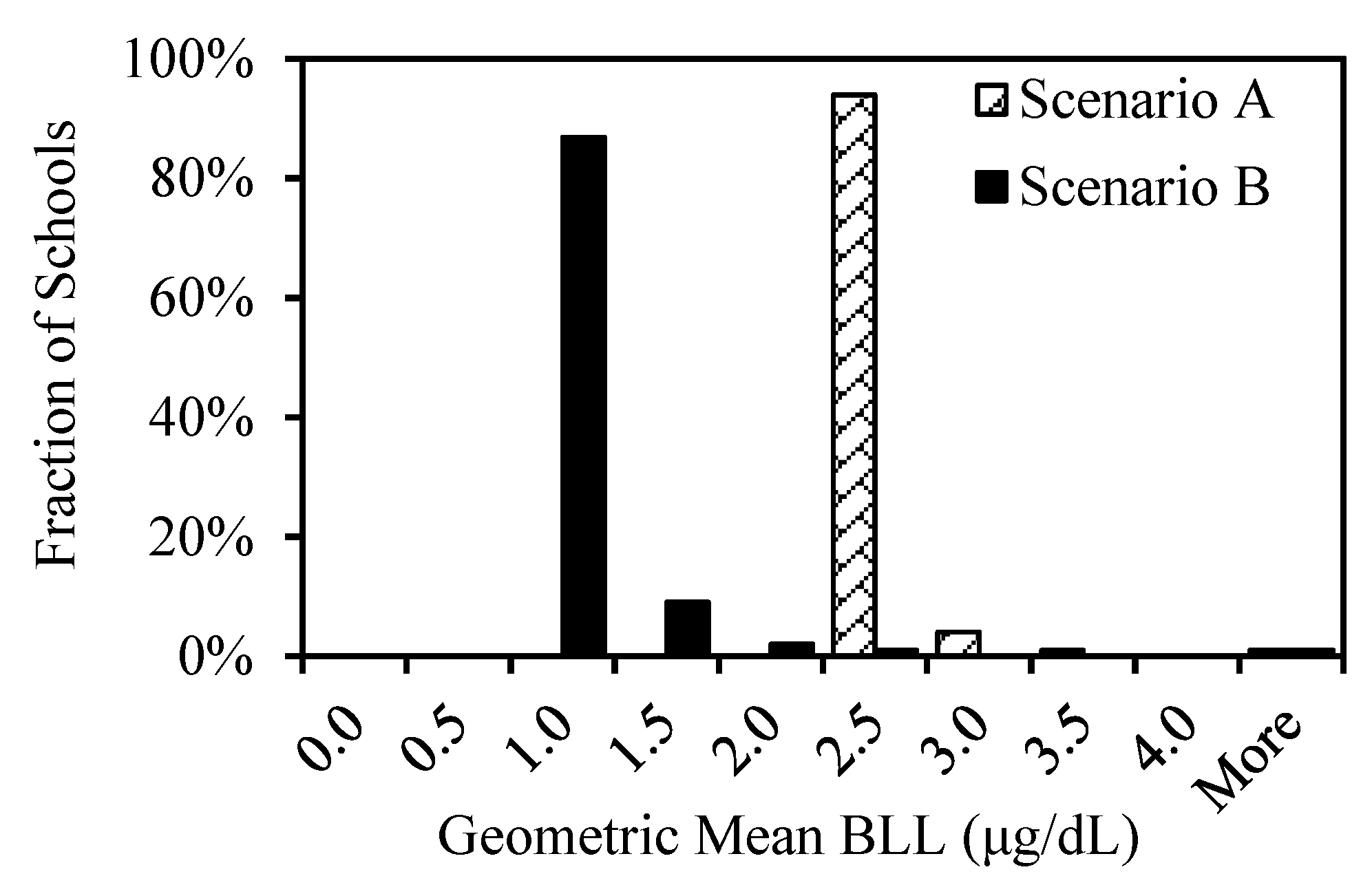
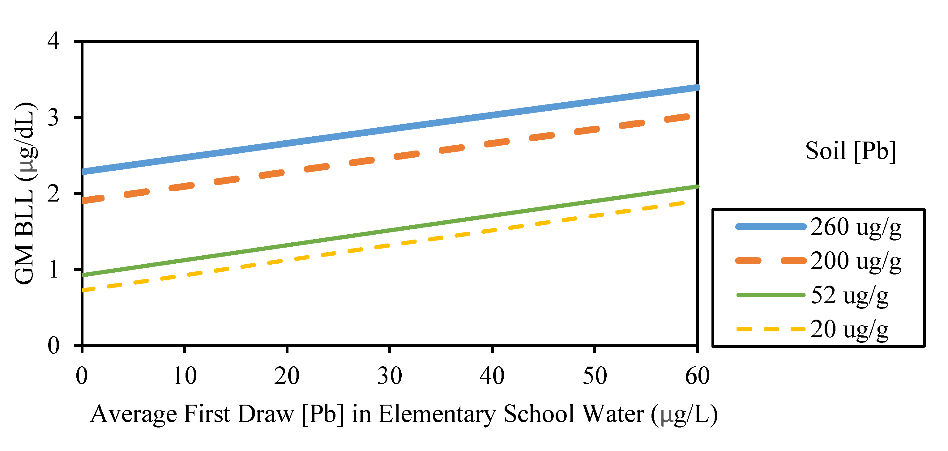
3.2.1. Geometric Mean BLL

As shown in Figure 1, scenario A (using the 90th percentile soil lead concentration) predicted 94% of the elementary schools tested in 2019 (93 schools) to have students with a mean BLL of approximately 2.5 μg/dL while scenario B (using the median soil lead concentration) predicted 87% of these schools (86 schools) to have students with a mean BLL of approximately 1.0 μg/dL. Both scenarios predicted a single elementary school to have students with a geometric mean BLL greater than the recommended BLL limit of 5 μg/dL. Both distributions have prominent peaks and are skewed to the right. The prominent peaks indicate that only a few schools had student populations with geometric means outside of the most-predicted value. However, the positive skew indicates that these few outlying schools have populations with significantly greater BLLs than most schools. Also, scenario A’s distribution is shifted significantly to right of scenario B’s distribution. In other words, almost all the geometric means predicted by scenario A are substantially greater than those predicted by scenario B. This highlights the importance of employing the appropriate site-specific soil lead concentration into the IEUBK model. Although previous authors targeted other geographic locations and thus employed different lead concentrations in both soil and water, the results obtained herein are similar to their findings. The previous study’s model predicted elementary schools in Seattle to have a typical scenario geometric mean BLL ranging between 1.6 μg/dL and 2.5 μg/dL and a worst-case scenario geometric mean BLL ranging between 1.7 μg/dL and 5.0 μg/dL [25]. These values are comparable to this study’s findings for scenarios B and A, respectively.

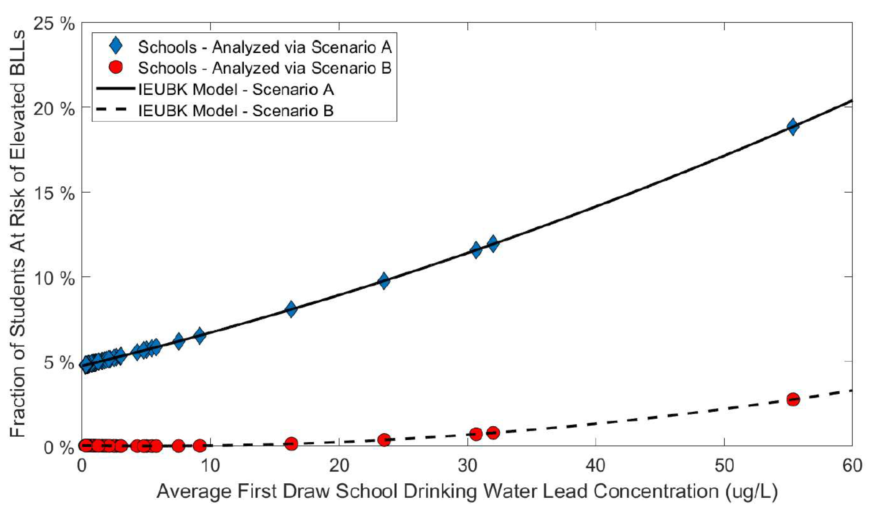
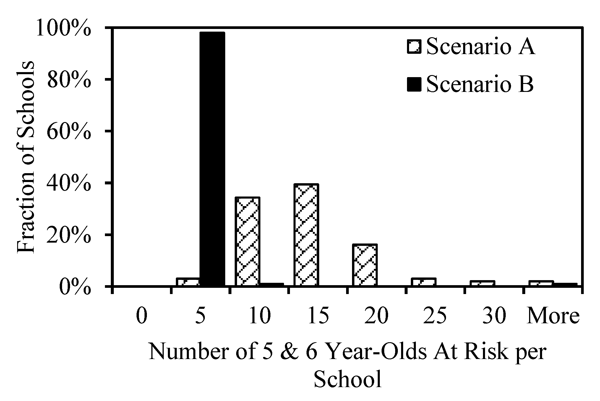
3.2.2. Percentage and Number of At-Risk Students

All but 6 of the 99 tested elementary schools had average first draw drinking water lead concentrations less than 15 μg/L. Figure 2 depicts the projected fraction of at-risk students as a function of the school drinking water lead concentration for scenarios A and B. Although both scenarios indicate that the fraction of at-risk students would increase as the water lead concentration increases, scenario A projects a more rapid increase and thus a larger at-risk population for equivalent water lead concentrations. Additionally, scenario A predicts significantly more at-risk students when water lead concentrations are minimal. These two trends—a more rapid increase and a larger initial percentage—show how the estimated fraction of at-risk students is highly sensitive to the input soil lead concentration. The diamond and circle markers on Figure 2 represent the schools where the readings were taken. The average first draw school drinking water lead concentration is represented on the horizontal axis and each school’s projected fraction of at-risk students is represented on the vertical axis. Since its water lead concentration was two orders of magnitude greater than that of the school with the next highest reading, the outlying school is not depicted on Figure 3. Since it had an average first draw drinking water lead concentration over 1000 μg/L, the outlier far exceeds the upper bound of Figure 2’s horizontal axis (60 μg/L). Both scenarios A & B projected nearly 100% of this outlying school’s 5- and 6-year-olds to be at risk of elevated BLLs. These drinking water lead concentrations compare well to measurements taken in other studies for other school districts. As other authors have concluded, a large cluster of schools had minimal lead concentrations in the drinking water while a few schools had exceptionally high values [27,31].
The at-risk population distribution is depicted in Figure 3. The figure shows the number of at-risk 5- and 6-year-olds at each school. Scenario B had a sharp peak and thus estimated 98% of schools had 5 or fewer 5- and 6-year-olds at risk of elevated BLLs. However, scenario A had a positively skewed wide distribution. Scenario A estimated a plurality of schools (39%) to have approximately 15 students at risk of elevated BLLs and 7% of schools to have over 20 students at risk. Scenarios A and B place the outlying elementary school (having an average first draw drinking water lead concentration exceeding 1000 μg/L) in the final column of Figure 3 since nearly 100% of the school’s 5- and 6-year-olds (approximately 120 students) were projected to be at risk according to both scenarios.

3.3. Secondary School Assessment

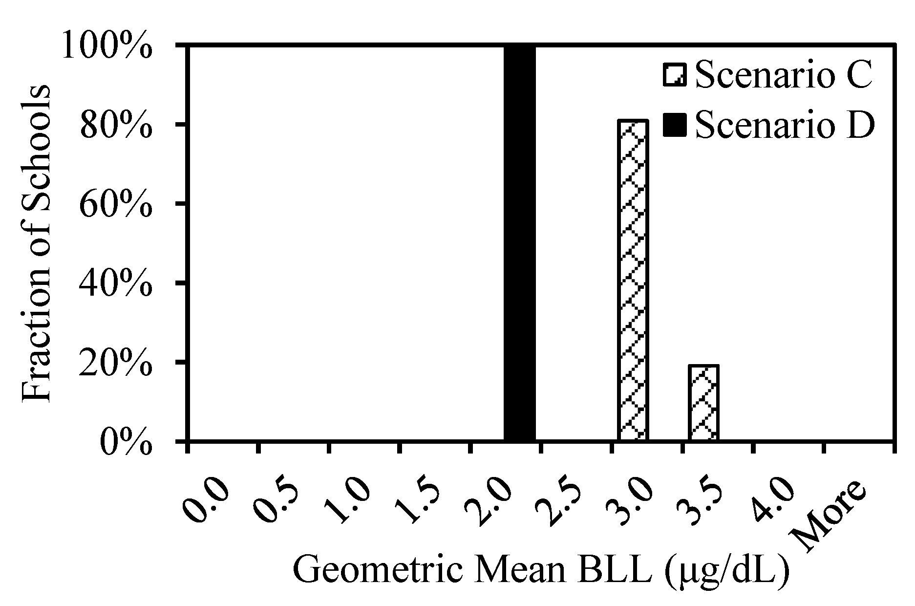
3.3.1. Geometric Mean BLL

As shown in Figure 4, scenario C (using the 90th percentile soil lead concentration) estimated that 81% of the secondary schools tested in 2019 (55 schools) had student populations with a geometric mean BLL of approximately 3.0 μg/dL and the remaining 19% of these schools (13 schools) had populations with a geometric mean BLL of approximately 3.5 μg/dL. Scenario D (using the median soil lead concentration) estimated that all 68 of these schools had a geometric mean BLL of approximately 2.0 μg/dL. Neither scenario predicted any schools having students with a geometric mean greater than the recommended BLL limit (5 μg/dL). Both scenario distributions have prominent peaks and no outliers. This indicates that no schools had populations with geometric means far outside of the most-predicted value. Scenario C’s values are shifted significantly to right of scenario’s D’s values meaning all the geometric means estimated by scenario C are substantially greater than those estimated by scenario D. It is detailed in the discussion that this shift resulted from the difference in baseline BLL input, not the difference in soil lead concentration input (as was the reason for the difference between the scenario A and B distributions).

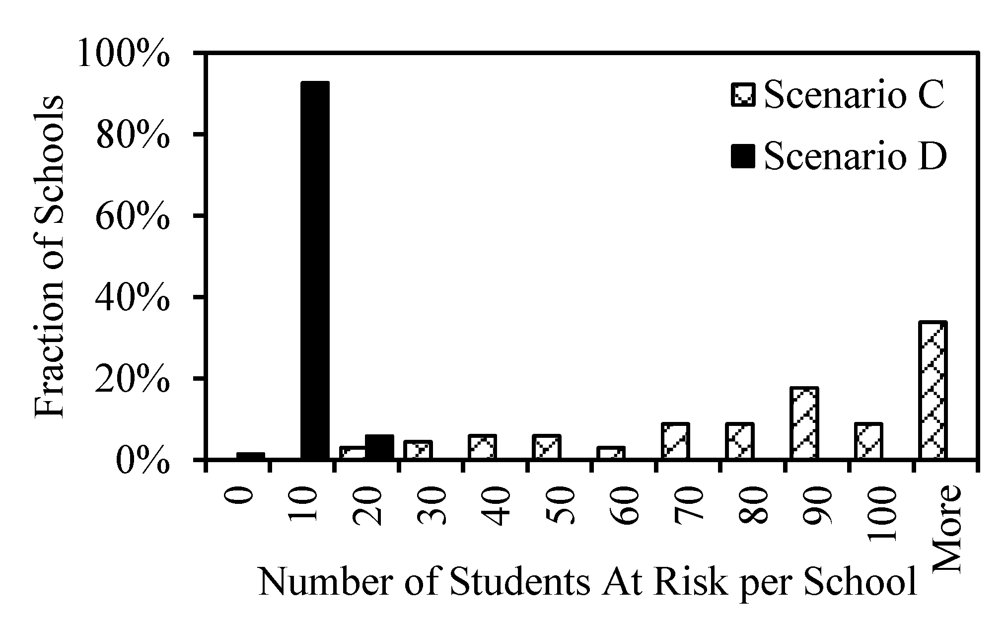
3.3.2. Percentage and Number of At-Risk Students

All but one of the 68 secondary schools tested in 2019 had average first draw drinking water lead concentrations less than 15 μg/L. Figure 5 depicts the projected percentage of at-risk students as a function of the school drinking water lead concentration for scenarios C and D. Both scenarios show the fraction of at-risk students increasing as the water lead concentration increases but scenario C projects a slightly more rapid increase. The majority of the difference between scenarios C and D resulted from the large initial difference. At negligible drinking water lead concentrations, scenario C predicts over 13% of students to be at risk while scenario D predicts less than 1% of students to be at risk. This difference is mainly attributed to the baseline BLL input in Bowers’ model (obtained from the IEUBK model), not the soil lead concentration to which secondary students were exposed. This further emphasizes the need for site-specific lead concentration data to be used in the IEUBK model and introduces the notion that minimizing BLL concentrations in adult populations is best achieved by minimizing lead exposure during childhood.
Considering the number of at-risk 11- to 17-year-old students ( N ( 11 17 ) i ) for each school, the school at-risk population distribution is depicted in Figure 6. The figure shows the number of at-risk students at each school. Scenario D had a sharp peak and thus estimated 93% of schools to have approximately 10 students at risk of elevated BLLs. However, scenario C had a nearly uniform distribution with 78% of the schools having at least 60 students at risk.

4. Discussion

4.1. Elementary School Assessment
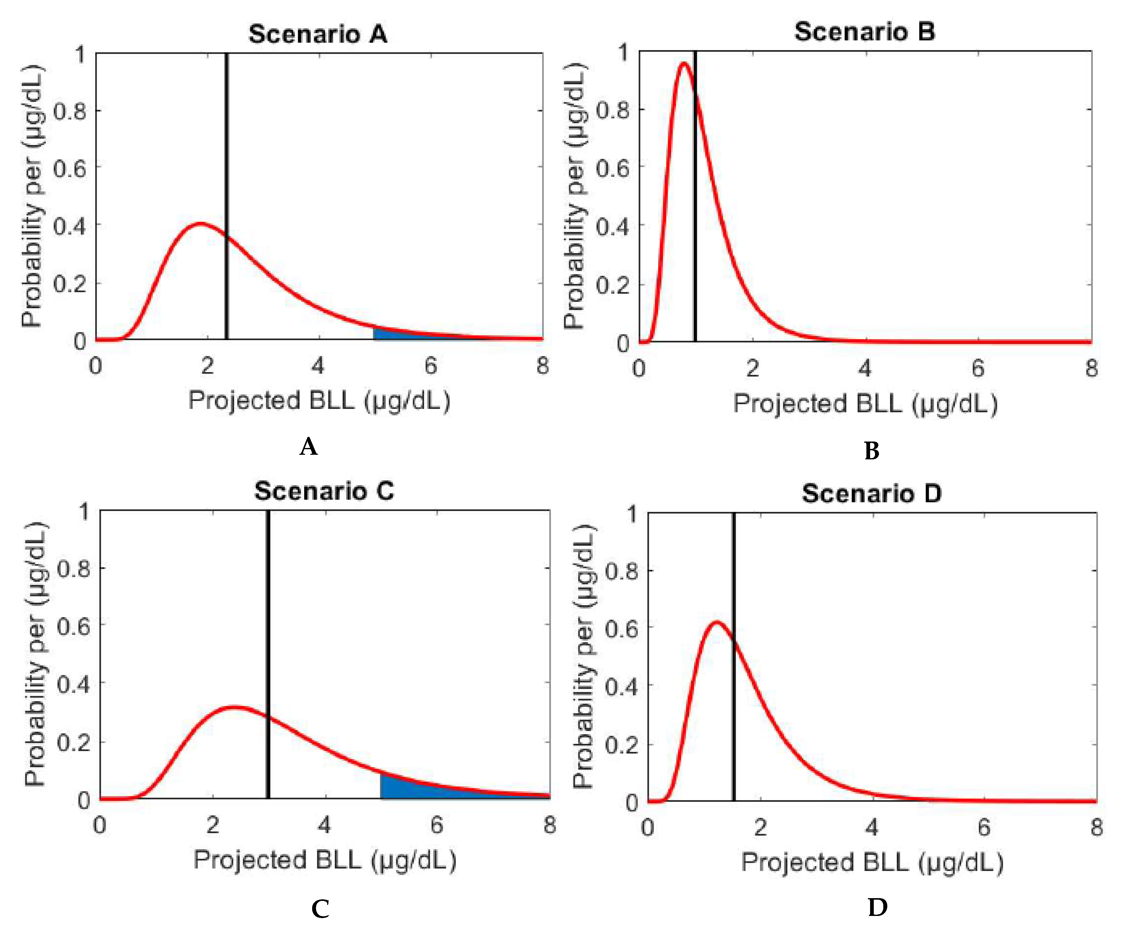
4.1.1. Scenario A

Scenario A projected all schools to have at least 4.8% of the students being at risk of elevated BLLs. This included schools with minimal lead concentrations in the drinking water. In other words, because the input soil lead concentration was the region’s 90th percentile value, all schools had at least 1 in 21 students at risk of an elevated BLL. Applying a linear approximation to scenario A in Figure 2, the fraction of at-risk students increased at a rate of 0.20% per μg/L. Since this rate of increase is relatively small, schools with low or mid-range water lead concentrations would benefit more from mitigating the lead in the soil rather than mitigating the lead in the water. Specifically, for schools with average first draw water lead concentrations less than the recommended upper limit of 15 μg/L [18], further reducing the drinking water lead concentration would result in only an incremental reduction of at-risk students. For these schools, high BLLs among students are most likely attributed to the high soil lead concentration—not the drinking water lead concentration. However, there were six elementary schools with average drinking water lead concentrations greater than 15 μg/L. Using scenario A, these schools had at least 8% of their 5- and 6-year-olds at risk of BLLs above 5 μg/dL. Of these six schools, one had approximately 100% of its students at risk because its average water lead concentration was greater than 1000 μg/L. The other five schools ranged from 16 μg/L (8% of students at risk) to 55 μg/L (19% of students at risk). For these schools, reducing the water lead concentration to below 15 μg/L could substantially reduce the fraction of at-risk students. A lognormal distribution depicting scenario A is shown in Figure 7A. Scenario A predicted the weighted geometric mean BLL across all the region’s 5- and 6-year-olds to be 2.35 μg/dL. This value is depicted by the vertical line in Figure 7A. Approximately 1300 of the estimated 22,300, 5- and 6-year-old students were projected to have BLLs above 5 μg/dL. The shaded area (5.8% of the total area) in Figure 7A represents this fraction of students. Remediating the high lead concentration in water at the one outlying school would prevent approximately 120 of the region’s estimated 22,300 (0.5%) 5- and 6-year-old students from being at risk of elevated BLLs.
Although these data represent the conditions at each school for the fall of 2019, it should be noted that 40 of the 99 elementary schools had drinking water samples analyzed for lead during 2017 as well. Although it is unknown which remediation efforts (if any) were implemented after the 2017 sampling, 33 of the 40 elementary schools exhibited no significant difference in water lead concentration between the 2017 data and the 2019 data. Of the remaining 7 schools, 3 exhibited a decrease in water lead concentration whereas 4 exhibited an increase. Only 1 of these schools had an average water lead concentration greater than 15 μg/L in 2017 but all 4 of these schools were beyond this recommended limit in 2019 (although 6 elementary schools had average water lead concentrations greater than 15 μg/L in 2019, 2 of these were not tested in 2017). This demonstrates the need for continual testing. A school may have acceptable values at one timepoint, but it might not maintain a low water lead concentration.
The results obtained for scenario A parallel those of other authors. The previous study of Seattle public schools indicated that approximately 11% of the students attending “typical exposure schools” (schools having median first-draw drinking water lead concentrations of 6 μg/L) were at risk of elevated BLLs before remediation and scenario A predicted approximately 7% of these students would be at risk. Likewise, for students attending a “low exposure school” (having a median first-draw drinking water lead concentration of 0.5 μg/L), the previous study suggested that approximately 7% of students would be at risk while scenario A predicted 5% of students to be at risk. Both the previous study and scenario A indicate that schools with high initial lead concentrations will experience the greatest decrease in fraction of at-risk students when remediation efforts are implemented. Also, because lead was present in other media, both predict approximately 5% of students to be at risk regardless of the lead concentration in the school drinking water [27].

4.1.2. Scenario B

Scenario B estimated very few students to be at risk of elevated BLLs for the majority of schools. Of the six schools with average water lead concentrations above 15 μg/L, four were projected to have less than 1% of their students at risk, one was projected to have 3% of its students at risk, and the extreme outlier was projected to have approximately 100% of its students at risk. When employing scenario A, these same schools were modeled to have approximately 10%, 19%, and 100% at risk, respectively. Aside from the extreme outlier, scenario B not only predicted significantly fewer students to be at risk than scenario A, it predicted very few students to be at risk in general. For scenario B, the percentage of at-risk students increased at a rate of only 0.05% per μg/L over the region depicted in Figure 2. A lognormal distribution depicting scenario B is shown in Figure 7B. Scenario B predicted the weighted geometric mean BLL across all the region’s 5- and 6-year-olds to be 0.99 μg/dL. This value is depicted by the vertical line in Figure 7B. Since the distribution is lognormal, half of the students would have BLLs greater than this value while half would have BLLs less this value. Approximately 140 of the estimated 22,300 (0.6%), 5- and 6-year-olds were projected to have BLLs above the recommended limit (5 μg/dL). Since the limit is well above the geometric mean, the area in Figure 7B representing this fraction is not visible. Approximately 88% of the 140 at-risk children were students at the single outlying school. In other words, remediation efforts at this school alone could prevent approximately 120 students from being at risk and would decrease the total percentage of at-risk 5- and 6-year-olds to an indiscernible value.

4.1.3. Comparison of Scenarios A & B

Aside from the extreme outlier, scenario A’s lowest at-risk percentage (4.8% for several schools with minimal average drinking water lead concentration) was almost double scenario B’s highest at-risk percentage (3% for the school with an average drinking water lead concentration of 55.4 μg/L). Since scenarios A and B assumed all students were exposed to the region’s 90th percentile and median soil lead concentrations, respectively, scenario A may overestimate the percentage of at-risk students while scenario B may underestimate it. However, as stated above, these scenarios can be interpreted as probabilities of individual risk, in addition to percentages of at-risk populations. In other words, scenario A can be interpreted as the probability that a typical student who is exposed to the region’s 90th percentile soil lead concentration will have an elevated BLL. Viewing scenario A from this perspective, Figure 2 shows that this typical student would have an 8% chance of having an elevated BLL when exposed to an average school drinking water lead concentration of 15 μg/L. Furthermore, for the 10% of students who are exposed to soil lead concentrations exceeding the 90th percentile value, the chance of an elevated BLL while attending a school adhering to the 15 μg/L upper limit would be exponentially greater than 8%. Therefore, for individual probability estimates, it is recommended to employ both scenarios A and B depending on application and it is recommended to use site-specific soil lead concentrations to ensure accurate predictions within these bounds. For reference, the median soil lead concentration for the region studied was approximately 3 times greater than the national naturally occurring median soil lead concentration of 18.1 μg/g [48].

4.2. Secondary School Assessment
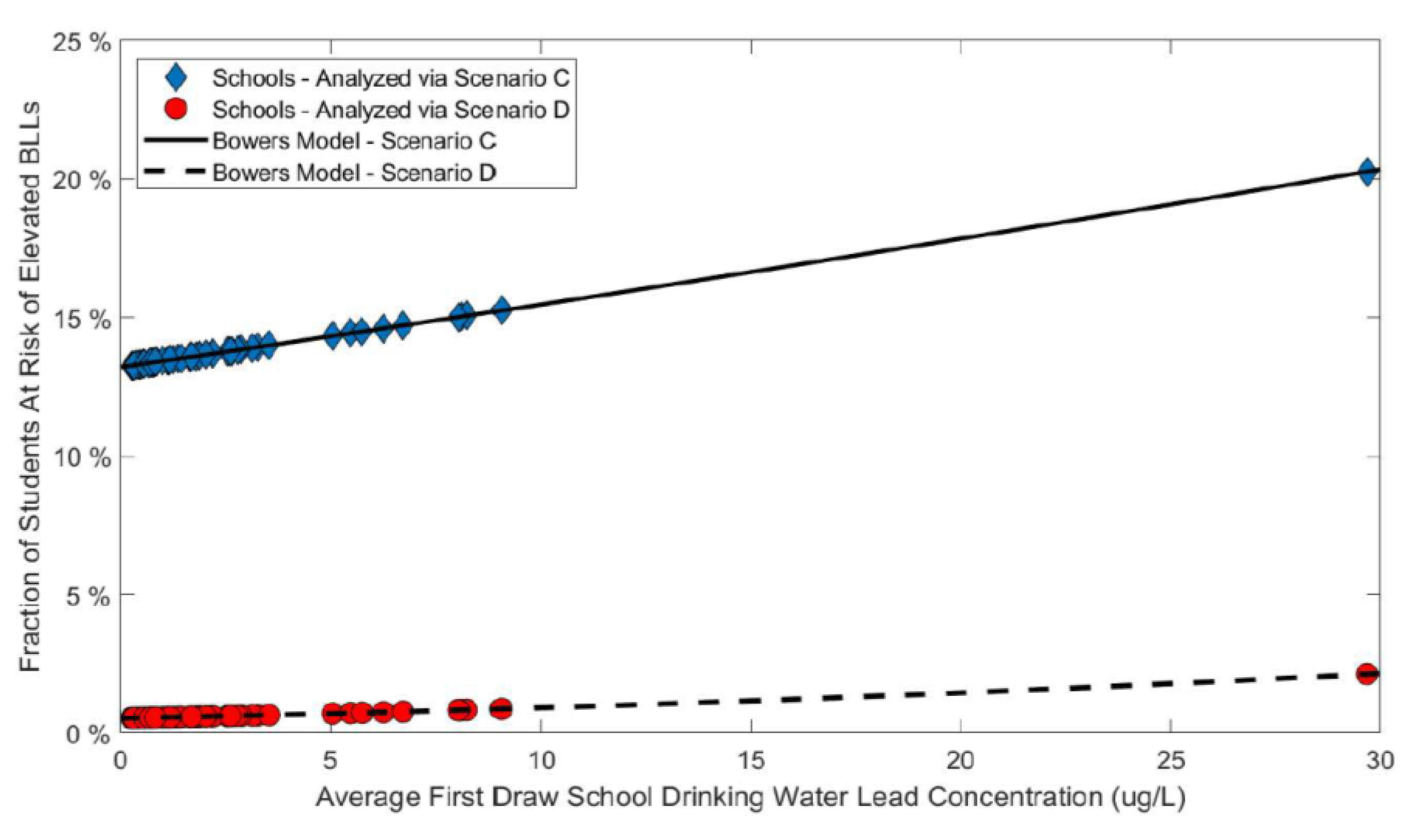
4.2.1. Scenario C

Scenario C projected each school to have at least 13.2% of its students to be at risk of having elevated BLLs. This included schools with minimal lead concentrations in the drinking water. In other words, because the soil lead concentration and the BLL baseline were high for scenario C, all schools were projected to have at least 1 in 8 students at risk of an elevated BLL. Applying a linear approximation to scenario C in Figure 6, the fraction of at-risk students increased at a rate of 0.23% per μg/L. As was the case for scenario A, since this rate of increase is relatively small, schools with low or mid-range water lead concentrations would benefit more from mitigating the lead in the soil rather than mitigating the lead in the water. One school had an average water lead concentration of 30 μg/L and thus was projected to have approximately 20% of its students at risk of elevated BLLs. For this school, reducing the water lead concentration to below the 15 μg/L limit could substantially reduce the fraction of at-risk students. A lognormal distribution depicting scenario C is shown in Figure 7C. Scenario C predicted the weighted geometric mean BLL across all the region’s secondary school students to be 2.99 μg/dL. This value is depicted by the vertical line in Figure 7C. Approximately 6900 of the estimated 50,800 secondary school students were projected to have BLLs above 5 μg/dL. The shaded area (13.6% of the total area) in Figure 7C represents this fraction of students.
Analogous to the elementary schools, a fraction of the secondary schools had drinking water samples analyzed for lead during 2017. Of the 68 secondary schools tested in 2019, 32 were also tested in 2017. Although it is unknown if any remediation efforts were implemented between 2017 and 2019, none of these 32 secondary schools exhibited an increase in water lead concentration between the testing years. On the contrary, 3 schools exhibited significant decreases and the remaining 29 schools exhibited no significant change. All 3 schools exhibiting a reduction had average first draw drinking water lead concentrations greater than the recommended upper limit (15 μg/L) in 2017 but substantially below this limit in 2019. The school having a concentration above the limit in 2019 was not tested in 2017.

4.2.2. Scenario D

Scenario D predicted very few students to be at risk of elevated BLLs for the majority of schools. Scenario D not only predicted significantly fewer students at risk compared to scenario C, it estimated very few students to be at risk in general. Applying a linear approximation to scenario D in Figure 5, the fraction of at-risk students increased at a rate of 0.05% per μg/L. For the school with an average water lead concentration of 29.7 μg/L, only 2.1% of its students were at risk of elevated BLLs (compared to 20% via scenario C). A lognormal distribution depicting scenario D is shown in Figure 7D. Scenario D predicted the weighted geometric mean BLL across all the region’s secondary school students to be 1.53 μg/dL. This value is depicted by the vertical line in Figure 7D. Approximately 300 of the estimated 50,800 (0.6%) secondary school students were projected to have BLLs above the recommended limit of 5 μg/dL. Since this limit is well above the geometric mean, the area in Figure 7D representing this fraction is not visible.

4.2.3. Comparison of Scenarios C & D

The percent of at-risk students was significantly lower for all schools when employing scenario D as compared to scenario C. Scenario C’s lowest estimated percentage (13.2% for several schools with minimal average drinking water lead concentration) was over 6 times scenario D’s highest estimated percentage (2.1% for the school with an average water lead concentration of 29.7 μg/L). This indicated that scenario D may underestimate the percentage of at-risk students whereas scenario C may overestimate the percentage of at-risk students. However, the large difference between scenarios C & D is derived from the baseline BLL input, not the difference in soil lead concentration exposure (as was the case for scenarios A & B). In other words, students with elevated BLLs during elementary school have significantly increased risks of elevated BLLs during secondary school, even if they reduce their exposure to lead during secondary school. This is initially apparent by inspection of the distribution of BLLs in Figure 4. Although a wide range of average first draw lead concentrations were measured in the secondary schools, the modeled BLLs had a very narrow distribution. This effect is best demonstrated by employing Bowers’ model using the individual probability interpretation in the two examples provided in Section 2 of the supplemental file. The two examples demonstrate that lead mitigation during secondary school (by either soil or water remediation) does not substantially narrow the gap between the two scenarios observed in Figure 6. According to Bowers’ model, if a student enters secondary school with a preexisting tendency to be at risk of an elevated BLL, he or she will continue to be at risk even if lead remediation efforts are implemented at the secondary school. Therefore, the primary focus for lead exposure mitigation should be at the elementary school level. If the student’s baseline BLL is high, the student has a high chance of being at risk even when the lead exposure has been mitigated during secondary school. In the school district studied, there were several elementary schools with average water lead concentrations above 15 μg/L, while there was only one secondary school exceeding this concentration.
In general, all four of the scenarios presented exhibit a continual rise in BLL. As exposure to lead continues over time (regardless of the source), the fraction of the population at risk of elevated BLLs also rises. All models approached a 100% chance for individuals having elevated BLLs when the population was exposed to very high lead concentrations in any medium. Efforts should be made to extrapolate these results to the region’s students of other ages. The IEUBK model targeted 5- and 6-year-olds while Bowers’ model targeted 11- to 17-year-olds. Since scenario A estimated the former population’s chance of risk to be approximately 5.8% while scenario C estimated the latter population’s chance of risk to be approximately 13.6%, a rudimentary interpolation would indicate that approximately 10% of 7- to 10-year-olds could be at risk of elevated BLLs (using the 90th percentile soil lead concentration). A similar method could be employed to interpolate between scenarios B and D.

4.3. Sensitivity Analysis

4.3.1. IEUBK Model

As indicated by previous authors [42] and the IEUBK guidance manual [20], the soil and dust lead concentrations are the most sensitive concentration parameters in the IEUBK model and thus require site-specific values for accurate modeling. This trend is depicted in Figure 8 below. The soil concentrations depicted in Figure 8 are representative of the concentrations referenced in this study. The lowest concentration, 20 μg/g, is approximately the median naturally occurring soil lead concentration in the United States [48] whereas the next concentration, 52 μg/g, is the median soil lead concentration in the school district [43]. The two elevated concentrations, 200 μg/g and 260 μg/g are the IEUBK model’s default soil concentration [36] and the school district’s 90th percentile value [43], respectively. The x-axis range compares with that of Figure 2’s to depict the average first draw drinking water lead concentrations in elementary schools. As observed in the data set populated on Figure 2, the median drinking water lead concentration in this study was 0.71 μg/L whereas the 90th percentile value was 5.45 μg/L. Therefore, Figure 8 represents the combinations of soil and water concentrations that are most likely to be observed for the given population. As the figure demonstrates over this most-common interval, the GM BLL increases at a rate of approximately 0.02 μg/dL for every 1 μg/L increase in average first draw drinking water lead concentration. This rate is consistent for all soil lead concentrations since all four trendlines exhibit the same constant slope. Additionally, the GM BLL increases at a rate of approximately 0.006 μg/dL for every 1 μg/g increase in soil lead concentration. Again, this rate is consistent over the range of interest since the trendlines are spaced solely according to their differences in soil concentration.
To understand the effects of these rates, the differences between the 90th percentile concentration and the median concentration was calculated for both soil and water. The 90th percentile soil concentration (260 μg/g) minus the median soil concentration (52 μg/g) yielded a 208 μg/g range in soil concentrations for the region. Likewise, 90th percentile average first draw drinking water concentration (5.45 μg/L) minus the median average concentration (0.71 μg/L) yielded a 4.74 μg/L drinking water concentration range. By multiplying the soil concentration range (208 μg/g) by the BLL soil rate (0.006 μg/dL per μg/g), the overall soil effect was calculated to be 1.2 μg/dL. Likewise, by multiplying the drinking water concentration range (4.74 μg/L) by the BLL drinking water rate (0.02 μg/dL per μg/L), the overall drinking water effect was calculated to be 0.1 μg/dL. Therefore, by observing these rates over the range of population data, it is clear that the soil concentration’s effect on BLL is 10 times greater than the drinking water’s effect on BLL for the population studied. In other words, with all other factors being equal, a student experiencing the 90th percentile drinking water concentration at school will have a BLL that is only 0.1 μg/dL higher than a student experiencing the median drinking water concentration at school. However, a student experiencing the 90th percentile soil lead concentration will have a BLL that is 1.2 μg/dL higher than a student experiencing the median soil lead concentration. This analysis demonstrates the need for site-specific soil lead concentrations when using the IEUBK to model BLLs from lead in drinking water. Fine adjustments (drinking water concentrations) to the model can only be implemented after broad parameters (soil lead concentrations) are accounted for. Also, this analysis demonstrates the importance of mitigating soil lead concentration levels at elementary schools. Although it is advisable for lead remediation efforts to be enacted for fixtures with extremely high drinking water lead concentrations, those efforts may be in vain if the soil lead concentrations of the region are high.

4.3.2. Bowers’ Model

In addition to the soil and water lead concentrations required by the IEUBK model, Bowers’ model requires the user to input the population’s preexisting BLL. The effects of this baseline BLL are displayed in Figure 9 below. The figure shows the model’s projections for GM BLL as a function of the secondary school’s average first draw drinking water lead concentration, the baseline BLL, and the soil lead concentration. The model projects the GM BLL to increase at a rate of 0.014 μg/dL for every 1 μg/L increase in drinking water lead concentration, to increase at a rate of 0.0005 μg/dL for every 1 μg/g increase in soil lead concentration, and to increase at a rate of 1 μg/dL for every 1 μg/dL increase in baseline BLL. Viewed from this perspective, it is apparent that the baseline BLL acts as a vertical shift of the projected BLL and has the most significant impact on the projected BLL. The soil lead concentration and the drinking water lead concentration have significantly less impact on the projected BLL. Therefore, when the Bowers’ model applies, soil and drinking water lead remediation efforts at secondary schools will have limited success in BLL reduction if the students enter the secondary schools with elevated BLLs. This is demonstrated by two examples in Section 2 of the supplementary file. This emphasizes the need to reduce the population’s BLL during elementary school (potentially via soil and drinking water lead remediation) to reduce the population’s BLL during secondary school. In general, Bowers’ model is intended for use among populations with low baseline BLLs and the baseline BLLs depicted in Figure 9 (2, 7, 12 μg/dL) are considered low according to the model [7]. Therefore, it is applicable for analysis herein.

4.4. Limitations

This study estimated the children’s blood lead levels using the drinking water lead concentration data acquired from one Tennessee school district. Several assumptions were employed in the models and therefore a thorough understanding of the study’s limitations is essential. As indicated above, the first draw school drinking water lead concentration was calculated as the arithmetic mean of all the sampled fixtures’ lead concentrations. In this calculation, each drinking water fixture was treated equally—regardless of its location within the school, frequency of use, or fixture type. Therefore, individual fixtures with high lead concentrations could significantly increase the average first draw school drinking water lead concentration. Thus, these outliers could disproportionally increase the predicted geometric mean BLL even though they may not frequently be used. Although this calculation could therefore bias the results to favor individual fixtures, all seven schools (6 elementary, 1 secondary) in this study with arithmetic means greater than 15 μg/L had multiple fixtures with lead concentrations greater than 15 μg/L. Thus, it is reasonable to deduce that no individual fixture had the sole effect on a school’s potentially high average drinking water lead concentration level. Furthermore, the method assumes all students consume half of their daily intake of water from school sources (distributed equally among all fixtures) and half from home sources. This assumption is similar to that of previous authors and corresponds well with those authors’ results [25,27]. However, if students are found to consume a different fraction of their water at school, or if they are found to favor one fixture over other another fixture, the geometric mean BLL would vary accordingly. Outside of modeling, other limitations involved the water sampling. Samples collected during the fall break had experienced extended stagnation whereas those collected before the school day had only been stagnant overnight. The longer stagnation period could have increased the lead concentration in the first draw water samples [49].

5. Conclusions

Two models were used to assess the risk of lead in school drinking water on students’ BLLs. The IEUBK model was used for 5- and 6-year-old students and Bowers’ model was used for 11- to 17-year-old students. Two scenarios, one employing the 90th percentile soil lead concentration and one employing the median soil lead concentration, were developed for each model. Site-specific lead concentrations were deemed critical to both models. The IEUBK model output was heavily dependent on the soil lead concentration input and the Bowers’ model output was heavily dependent on the IEUBK model output (baseline BLL). For elementary schools with low water lead concentrations, it may be more effective to mitigate the soil lead concentration than the water lead concentration to minimize the risk of elevated BLLs. Seven schools (6 elementary, 1 secondary) had an average water lead concentration above the recommended limit of 15 μg/L. It was projected that as much as 5.8% of 5- and 6-year-olds and 13.6% of 11- to 17-year-olds could be at risk of elevated BLLs. This equated to approximately 1300 and 6900 students in each age group, respectively. At the elementary school level, the two scenarios (high soil lead concentration and median soil lead concentration) yielded significantly different outputs due to the differences in soil lead concentration. However, at the secondary school level, the two scenarios yielded significantly different outputs due to the differences in baseline BLL inputs. This indicated that students with elevated BLLs during elementary school have significantly increased risks of elevated BLLs during secondary school, even if they reduce their exposure to lead during secondary school. Thus, it is recommended to focus efforts of lead remediation on elementary schools to minimize early exposure. As exposure to lead continues, the BLL increases. Therefore, the projected BLLs were higher for secondary school students than for elementary school students. The sensitivity analysis revealed the significant variations of estimated GM BLLs by the model input parameters and demonstrated the importance of site-specific data. Further research is suggested to identify the sources of lead release to the schools’ tap water and to develop the appropriate remediation practices. Future comparisons of the modeling predictions with actual lead blood levels for these student populations could be very illuminative.

Supplementary Materials

The following are available online at https://www.mdpi.com/2073-4441/12/6/1826/s1. Table S1: Populations of Students at Sampled Schools and Lead Mitigation in Secondary Schools—Examples.

Author Contributions

D.D. derived the model, performed analysis, prepared the manuscript original draft, and performed further editing. D.S. assisted with data collection, preparation, and preliminary analysis. M.S. acquired the data resources, devised the project and the main conceptual ideas, supervised the finding, and contributed into the writing by review and editing. All authors have read and agreed to the published version of the manuscript.

Funding

This research received no external funding.

Acknowledgments

The authors thank Joshua Tyler of the University of Memphis for his assistance with data processing. The authors also thank the administrators of the school district for assisting with the information.

Conflicts of Interest

The authors declare no conflict of interest.

References

  1. Li, Y.; Hu, J.; Wu, W.; Liu, S.; Li, M.; Yao, N.; Chen, J.; Ye, L.; Wang, Q.; Zhou, Y. Application of IEUBK model in lead risk assessment of children aged 61-84 months old in central China. Sci.Total Environ. 2016, 541, 673–682. [Google Scholar] [CrossRef] [PubMed]
  2. Jusko, T.; Henderson, C.R., Jr.; Lanphear, B.P.; Cory-Slechta, D.A.; Parsons, P.J.; Canfield, R.L. Blood Lead Concentrations <10 microg/dL and Child Intelligence at 6 Years of Age. Environ. Health Perspect. 2008, 116, 243–248. [Google Scholar] [CrossRef]
  3. Kwong, W.T.; Friello, P.; Semba, R. Interactions between iron deficiency and lead poisoning: Epidemiology and pathogenesis. Sci.Total Environ. 2004, 330, 21–37. [Google Scholar] [CrossRef] [PubMed]
  4. Miller, L.S.; Koplewicz, H.S.; Klein, R.G. Teacher Ratings of Hyperactivity, Inattention, and Conduct Problems in Preschoolers. J. Abnorm. Child Psychol. 1997, 25, 113–119. [Google Scholar] [CrossRef] [PubMed]
  5. Lanphear, B.P.; Dietrich, K.; Auinger, P.; Cox, C. Cognitive Deficits Associated with Blood Lead Concentrations <10 microg/dL in US Children and Adolescents. Public Health Rep. 2000, 115, 521. [Google Scholar] [CrossRef] [PubMed]
  6. Cleveland, L.M.; Minter, M.L.; Cobb, K.A.; Scott, A.A.; German, V.F. Lead hazards for pregnant women and children: Part 1: Immigrants and the poor shoulder most of the burden of lead exposure in this country. Part 1 of a two-part article details how exposure happens, whom it affects, and the harm it can do. Am. J. Nurs. 2008, 108, 40–49. [Google Scholar] [CrossRef]
  7. Bowers, T.S.; Beck, B.D.; Karam, H.S. Assessing the Relationship Between Environmental Lead Concentrations and Adult Blood Lead Levels. Risk Anal. 1994, 14, 183–189. [Google Scholar] [CrossRef]
  8. Salehi, M.; Jafvert, C.T.; Howarter, J.A.; Whelton, A.J. Investigation of the factors that influence lead accumulation onto polyethylene: Implication for potable water plumbing pipes. J. Hazard. Mater. 2018, 347, 242–251. [Google Scholar] [CrossRef]
  9. Jain, N.B.; Laden, F.; Guller, U.; Shankar, A.; Kazani, S.; Garshick, E. Relation between blood lead levels and childhood anemia in India. Am. J. Epidemiol. 2005, 161, 968–973. [Google Scholar] [CrossRef] [Green Version]
  10. Bryant, S.D. Lead-Contaminated Drinking Waters in the Public Schools of Philadelphia. J. Toxicol. Clin. Toxicol. 2004, 42, 287–294. [Google Scholar] [CrossRef]
  11. Cornelis, C.; Berghmans, P.; van Sprundel, M.; Van der Auwera, J. Use of the IEUBK Model for Determinination of Exposure Routes in View of Site Remediation. Hum. Ecol. Risk Assess. 2006, 12, 963–982. [Google Scholar] [CrossRef]
  12. Boyd, G.R.; Pierson, G.L.; Kirmeyer, G.J.; English, R.J. Lead variability testing in Seattle Public Schools. JAWWA 2008, 100, 53–64. [Google Scholar] [CrossRef]
  13. Subramanian, K.S.; Sastri, V.S.; Elboujdaini, M.; Connor, J.W.; Davey, A.B.C. Water Contamination: Impact of tin-lead solder. Water Res. 1995, 29, 1827–1836. [Google Scholar] [CrossRef]
  14. Ahamed, T.; Brown, S.P.; Salehi, M. Investigate the Role of Biofilm and Water Chemistry on Lead Deposition onto and Release from Polyethylene: An Implication for Potable Water Pipes. J. Hazard. Mater. 2020. [Google Scholar] [CrossRef]
  15. Salehi, M.; Li, X.; Whelton, A. Metal Accumulation in Representative Plastic Drinking Water Plumbing Systems. JAWWA 2017, 109, E479–E493. [Google Scholar] [CrossRef] [Green Version]
  16. Salehi, M.; Odimayomi, T.; Ra, K.; Ley, C.; Julien, R.; Nejadhashemi, A.P.; Hernandez-Suare, J.S.; Mitchell, J.; Shah, A.D.; Whelton, A. An investigation of spatial and temporal drinking water quality variation in green residential plumbing. Build. Environ. 2020, 169, 106566. [Google Scholar] [CrossRef]
  17. Salehi, M.; Abouali, M.; Wang, M.; Zhou, Z.; Nejadhashemi, A.P.; Mitchell, J.; Caskey, S.; Whelton, A.J. Case Study: Fixture Water Use and Drinking Water Quality in a New Residential Green Building. Chemosphere 2018, 195, 80–89. [Google Scholar] [CrossRef]
  18. Control of Lead and Copper. In 40 CFR 141.80-General Requirements; Legal Information Institute: Ithaca, NY, USA, 1991.
  19. Council on Environmental Health. Prevention of Childhood Lead Toxicity. In Pediatrics; American Association of Pediatrics: Itasca, IL, USA, 2016. [Google Scholar]
  20. EPA U.S. Guidance Manual for the Integrated Exposure Uptake Biokinetic Model for Lead in Children; US Environmental Protection Agency: Washington, DC, USA, 1994.
  21. Albalak, R.; Noonan, G.; Buchanan, S.; Flanders, W.D.; Gotway-Crawford, C.; Kim, D.; Jones, R.L.; Sulaiman, R.; Blumenthal, W.; Tan, R.; et al. Blood lead levels and risk factors for lead poisoning among children in Jakarta, Indonesia. Sci. Total Environ. 2003, 301, 75–85. [Google Scholar] [CrossRef]
  22. Schwartz, J. Low-level lead exposure and children’s IQ: A meta-analysis and search for a threshold. Environ. Res. 1994, 65, 42–55. [Google Scholar] [CrossRef]
  23. Zhang, X.-Y.; Carpenter, D.O.; Song, Y.-J.; Chen, P.; Qin, Y.; Wei, N.-Y.; Lin, S.-C. Application of the IEUBK model for linking Children’s blood lead with environmental exposure in a mining site, south China. Environ. Pollut. 2017, 231, 971–978. [Google Scholar] [CrossRef]
  24. Laidlaw, M.; Mohmmad, S.M.; Gulson, B.L.; Taylor, M.P.; Kristensen, L.J.; Birch, G. Estimates of potential childhood lead exposure from contaminated soil using the US EPA IEUBK Model in Sydney, Australia. Environ. Res. 2017, 156, 781–790. [Google Scholar] [CrossRef] [PubMed]
  25. Sathyanarayana, S.; Beaudet, N.; Omri, K.; Karr, C. Predicting Children’s Blood Lead Levels from Exposure to School Drinking Water in Seattle, Washington, USA. Ambul. Pediatr. 2006, 6, 288–292. [Google Scholar] [CrossRef] [PubMed]
  26. Zhong, B.; Giubilato, E.; Critto, A.; Wang, L.; Marcomini, A.; Zhang, J. Probabilistic modeling of aggregate lead exposure in children of urban China using an adapted IEUBK model. Sci. Total Environ. 2017, 584–585, 259–267. [Google Scholar] [CrossRef]
  27. Triantafyllidou, S.; Le, T.; Gallagher, D.; Edwards, M. Reduced risk estimations after remediation of lead (Pb) in drinking water at two US school districts. Sci. Total Environ. 2014, 466–467, 1011–1021. [Google Scholar] [CrossRef] [PubMed]
  28. Delgado-Caballero, M.R.; Valles-Aragón, M.C.; Millan, R.; Alarcón-Herrera, M.T. Risk Assessment Through IEUBK Model. in an Inhabited Area Contaminated with Lead. Environ. Prog. Sustain. Energy 2018, 37, 391–398. [Google Scholar] [CrossRef]
  29. Bowers, T.S.; Cohen, J.T. Blood Lead Slope Factor Models for Adults: Comparisons of Observations and Predictions. Environ. Health Perspect. 1998, 106 (Suppl. S6), 1569–1576. [Google Scholar] [CrossRef] [Green Version]
  30. Redmon, J.H.; Levine, K.E.; Aceituno, A.M.; Litzenberger, K.; Gibson, J.M. Lead in drinking water at North Carolina childcare centers: Piloting a citizen science-based testing strategy. Environ. Res. 2020, 183, 109126. [Google Scholar] [CrossRef]
  31. Deshommes, E.; Andrews, R.C.; Gagnon, G.; McCluskey, T.; McIlwain, B.; Doré, E.; Nour, S.; Prévost, M. Evaluation of exposure to lead from drinking water in large buildings. Water Res. 2016, 99, 46–55. [Google Scholar] [CrossRef]
  32. Costanza-Robinson, M.; Davis, G. Lead Levels in Drinking Water at Salisbury Community School, Salisbury VT. 2019. [Google Scholar]
  33. 40 CFR 141.86-Monitoring Requirements for Lead and Copper in Tap Water; Cornell Law School: Ithaca, NY, USA, 1991.
  34. Greatschools. Available online: https://www.greatschools.org/ (accessed on 21 November 2019).
  35. EPA U.S. IEUBK Model-Windows Version 1.1 Build 11; US Environmental Protection Agency: Washington, DC, USA, 2010.
  36. EPA U.S. Technical Support Document: Parameters and Equations Used in the Integrated Exposure Uptake Biokinetic Model for Lead in Children (v0.99d); US Environmental Protection Agency: Washington, DC, USA, 1994.
  37. EPA U.S. User’s Guide for the Integrated Exposure Uptake Biokinetic Model for Lead in Children (IEUBK) Windows; US Environmental Protection Agency: Washington, DC, USA, 2007.
  38. EPA U.S. Overview of the Clean Air Act and Air Pollution; US Environmental Protection Agency: Washington, DC, USA, 1990.
  39. MLGW. Memphis Water: Pure and Abundant Water Quality Report 2016; MLGW: Memphis, TN, USA, 2016; pp. 1–8. [Google Scholar]
  40. EPA U.S. A TRW Report: Review of a Methodology for Establishing Risk-Based Soil Remediation Goals for the Commerical Areas of the California Gulch Site; US Environmental Protection Agency: Washington, DC, USA, 1995.
  41. EPA U.S. EPA U.S. A TRW Report: Review of the EPA Uptake Biokinetic Model for Lead at the Butte NPL Site; US Environmental Protection Agency: Washington, DC, USA, 1992.
  42. Zartarian, V.; Xue, J.; Tornero-Velez, R.; Brown, J. Children’s Lead Exposure: A Multimedia Modeling Analysis to Guide Public Health Decision-Making. Environ. Health Perspect. 2017, 125. [Google Scholar] [CrossRef] [Green Version]
  43. Frederick, T.; Chan, S. EPA Tools and Resources Webinar: Urban. Background Study; US Environmental Protection Agency: Washington, DC, USA, 2018.
  44. WHO. Childhood Lead Poisoning 2010. Available online: https://www.who.int/ceh/publications/childhoodpoisoning/en/ (accessed on 25 June 2020).
  45. Lambrinidou, Y.; Triantafyllidou, S.; Edwards, M. Failing Our Children: Lead in U.S. School Drinking Water. New Solut. J. Environ. Occupat. Health Policy 2010, 20, 25–47. [Google Scholar]
  46. H.R.4939-Lead Contamination Control Act of 1988; United States Congress: Washington, DC, USA, 1988.
  47. Act to Amend Tennessee Code Annotated, Title 49; Title 68 and Title 69, Relative to Water Quality in Schools; Tennessee General Assembly: Nashville, TN, USA, 2018.
  48. Smith, D.B.; Cannon, W.F.; Woodruff, L.G.; Solano, F.; Kilburn, J.E.; Fey, D.L. Geochemical and Mineralogical Data for Soils of the Conterminous United States; U.S. Geological Survey: Reston, VA, USA, 2013.
  49. Proctor, C.; Rhoads, W.; Keane, T.; Salehi, M.; Hamilton, K.; Pieper, K.; Cwiertny, D.; Prevost, M.; Whelton, A. Considerations for Large Building Water Quality after Extended Stagnation. AWWA Water Sci. 2020, e1186. [Google Scholar] [CrossRef]
Figure 1. Distribution of BLL geometric means for elementary schools.
Water 12 01826 g001
Figure 2. Fraction of at-risk students vs. school water lead concentration.
Water 12 01826 g002
Figure 3. Distribution of at-risk population for elementary schools.
Water 12 01826 g003
Figure 4. Distribution of BLL geometric means for secondary schools.
Water 12 01826 g004
Figure 5. Fraction of at-risk students vs. water lead concentration at secondary schools.
Water 12 01826 g005
Figure 6. Distribution of at-risk population for secondary schools.
Water 12 01826 g006
Figure 7. (A)–(D). Probability density functions and geometric means for (A) Scenario A, (B) Scenario B, (C) Scenario C, (D) Scenario D. The plots represent the distribution of projected BLLs for (A & B) elementary school students using the IEUBK model and (C & D) secondary school students using Bowers’ model. Models of scenarios A & C employed the region’s 90th percentile soil lead concentration whereas models of scenarios B & D used the median soil lead concentration. The vertical line on each figure depicts the geometric mean of the distribution.
Water 12 01826 g007
Figure 8. Predicted geometric mean BLL as a function of both the elementary school average first draw drinking water lead concentration and the region’s soil lead concentration according to the IEUBK model.
Water 12 01826 g008
Figure 9. Predicted geometric mean BLL as a function of the secondary school average first draw drinking water lead concentration, the baseline BLL, and the region’s soil lead concentration according to bowers’ model.
Water 12 01826 g009
Table 1. Lead Concentration ([Pb]) in Water for a School District in Tennessee.
SchoolsElementary SchoolsMiddle SchoolsHigh Schools
201720192017201920172019
Schools sampled399916251736
Schools with [Pb] > 1 μg/L349013211334
Schools with [Pb] > 10 μg/L72605518
Schools with [Pb] > 15 μg/L52005416
Total sampled2701923112613118892
Fixtures with [Pb] > 15 μg/L2643014519
Maximum [Pb] (μg/L)5318,800914099285
Median [Pb] (μg/L)62273161230
Range (μg/L)<0.5–53<0.5–18,800<0.5–9<0.5–140<0.5–99<0.5–285

