Assessing the Fish Stock Status in Lake Trichonis: A Hydroacoustic Approach


Abstract
:1. Introduction
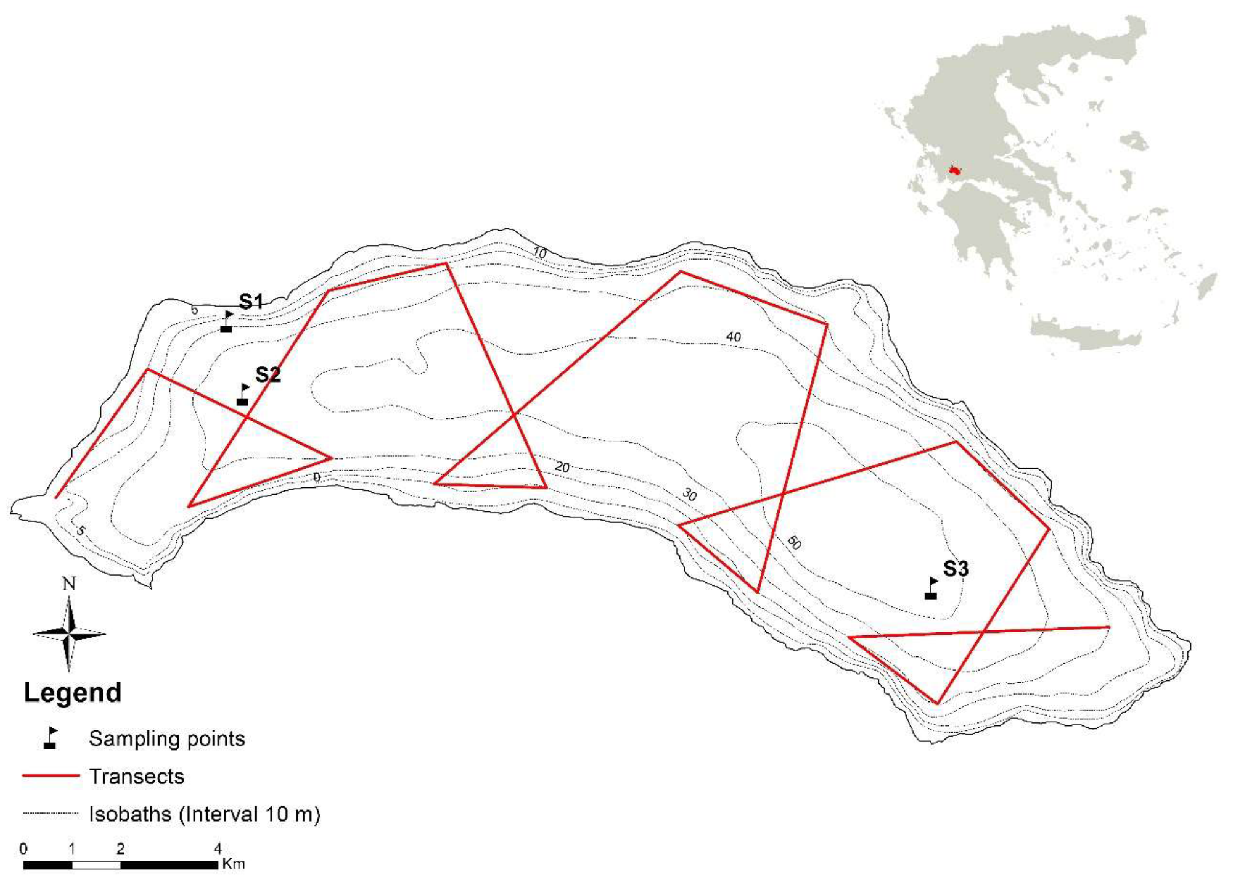
2. Study Area
3. Materials and Methods
3.1. Hydroacoustic Survey Design
3.2. Hydroacoustic Data Processing
3.3. Environmental Parameters
3.4. Statistical Analysis
4. Results
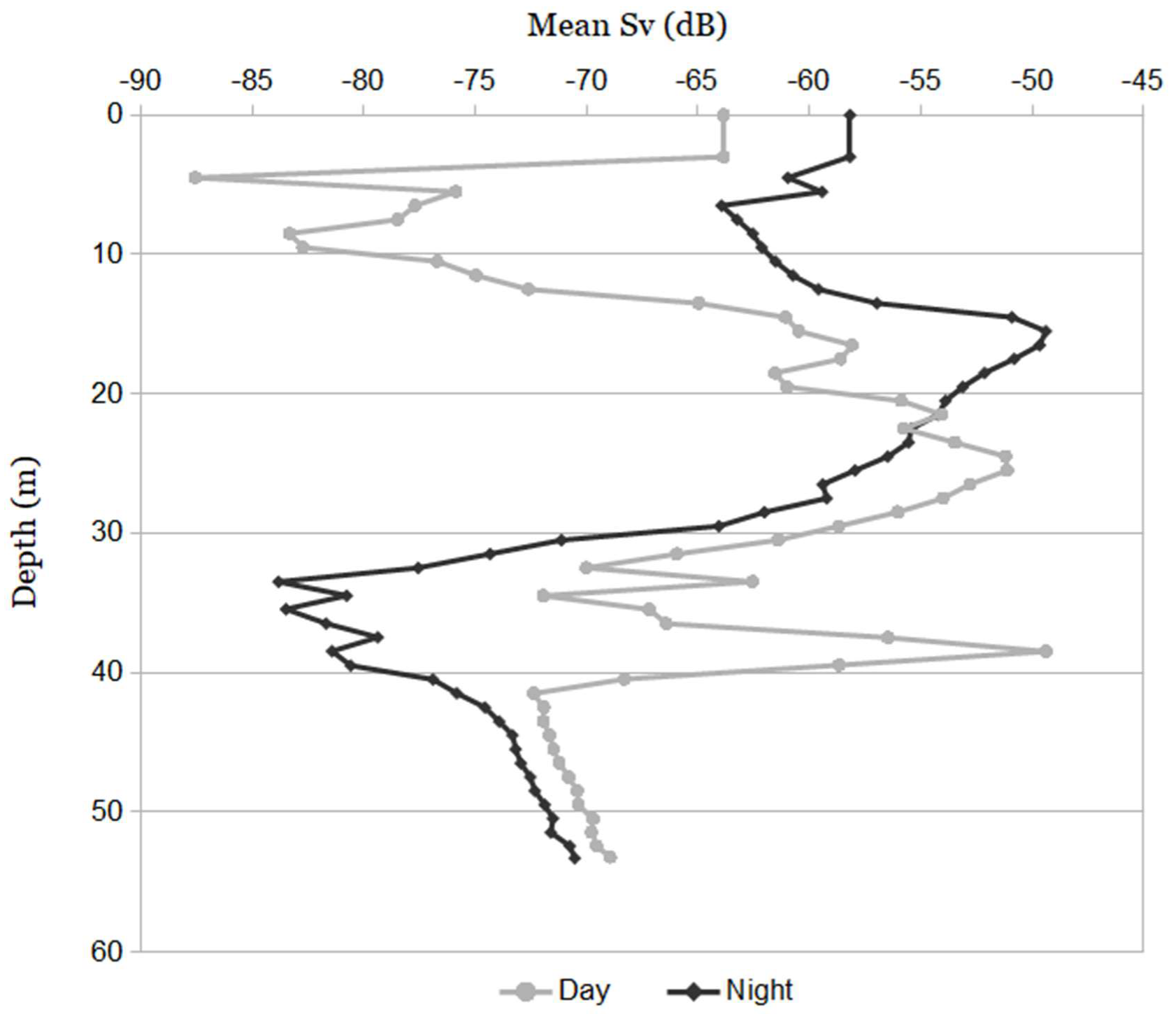
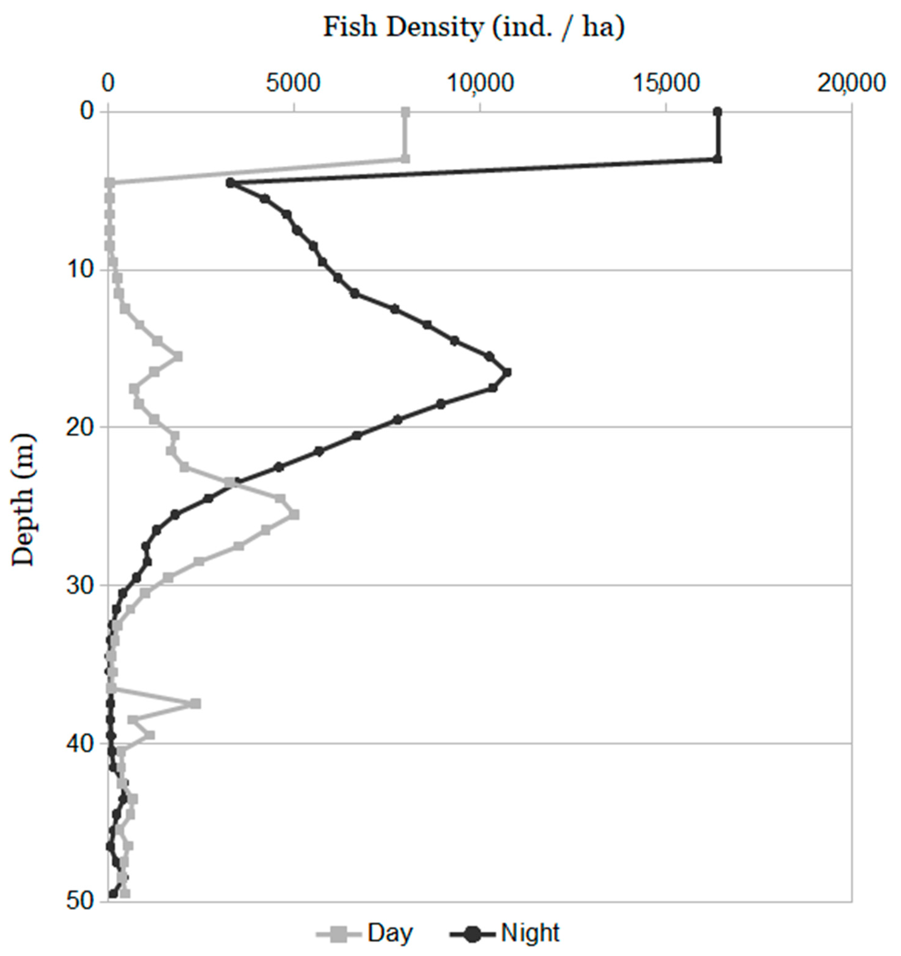
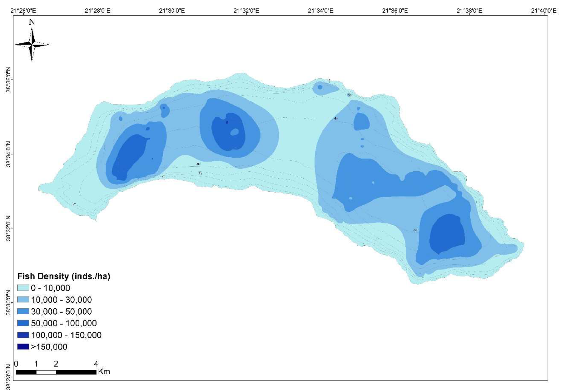
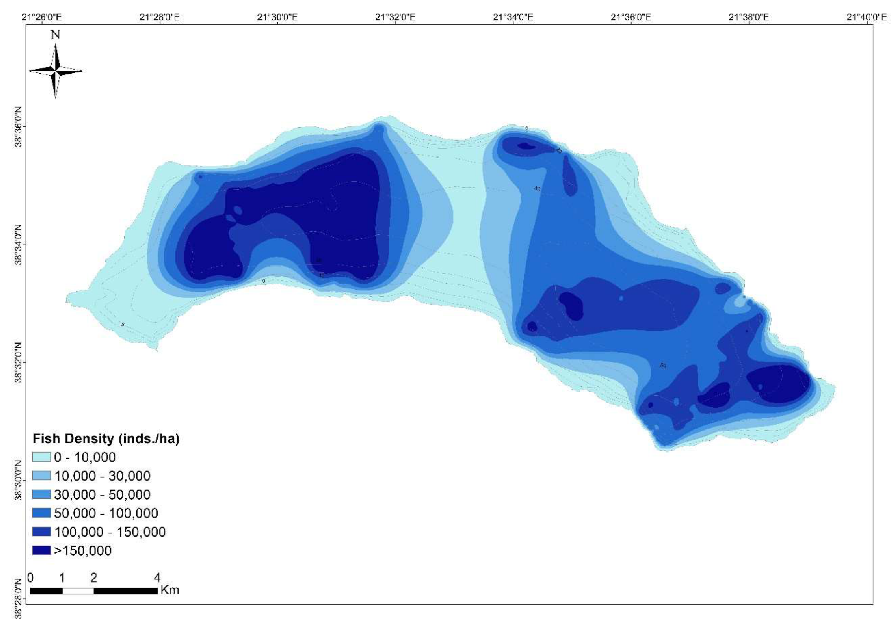
4.1. Acoustic Biomass and Fish Density
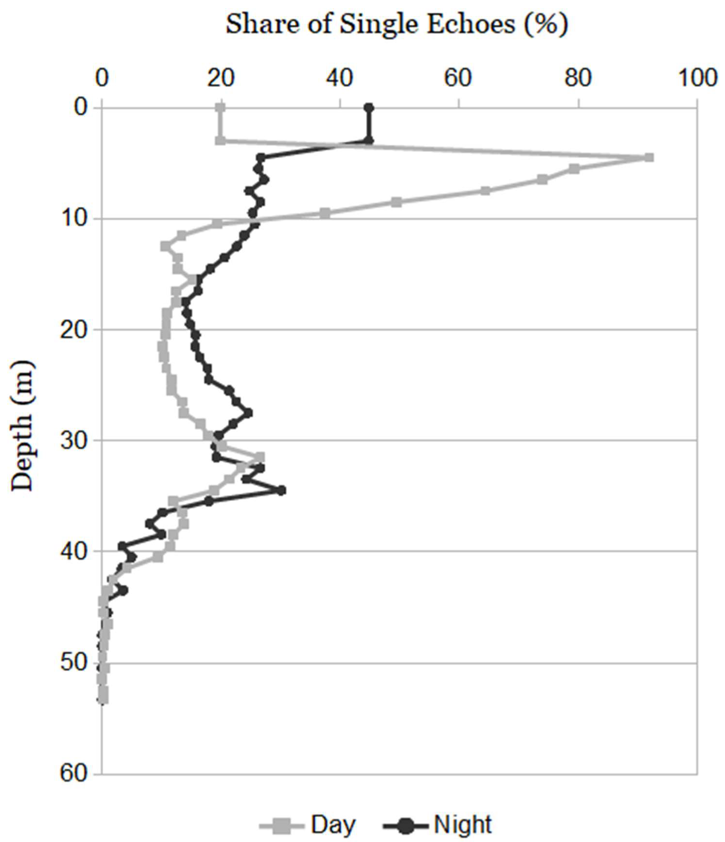
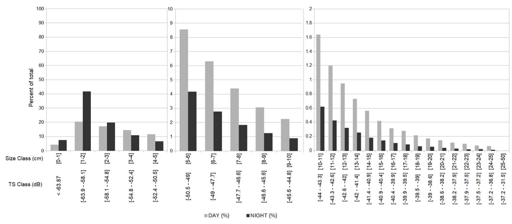
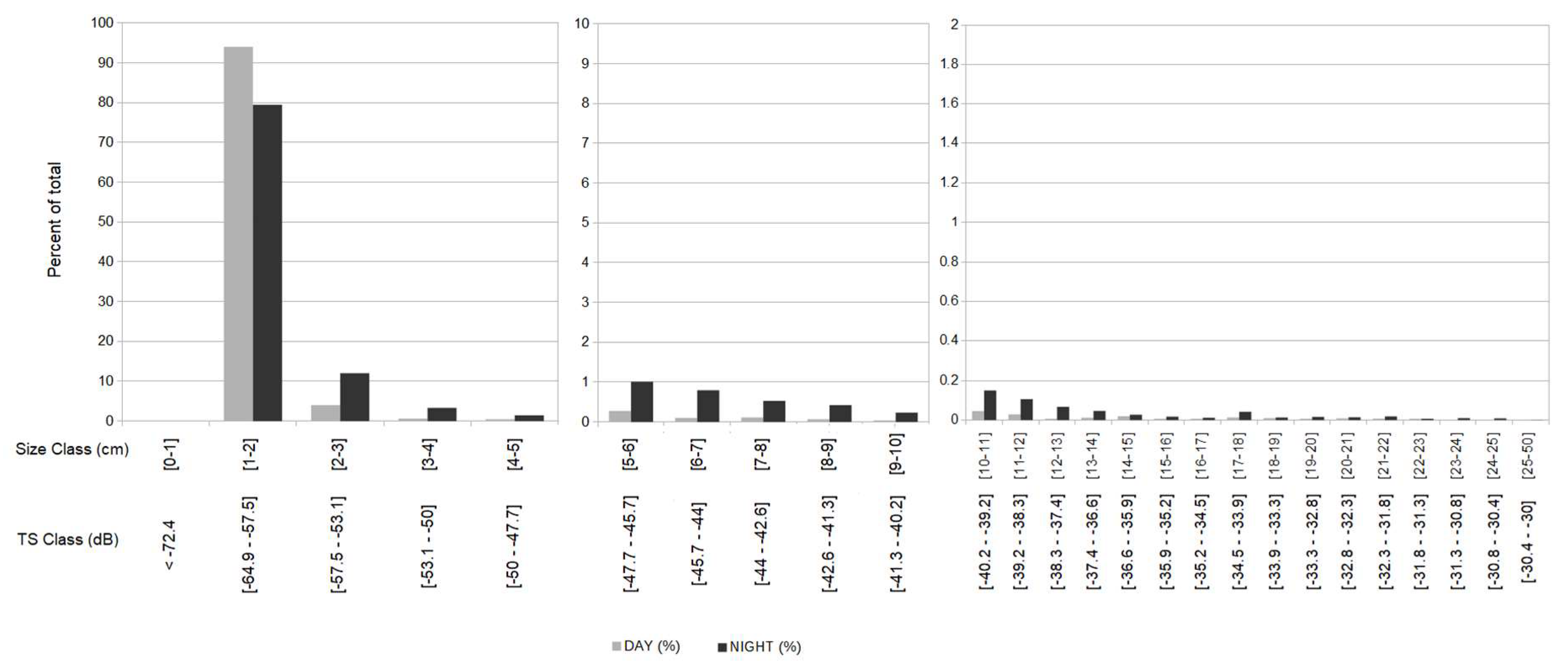
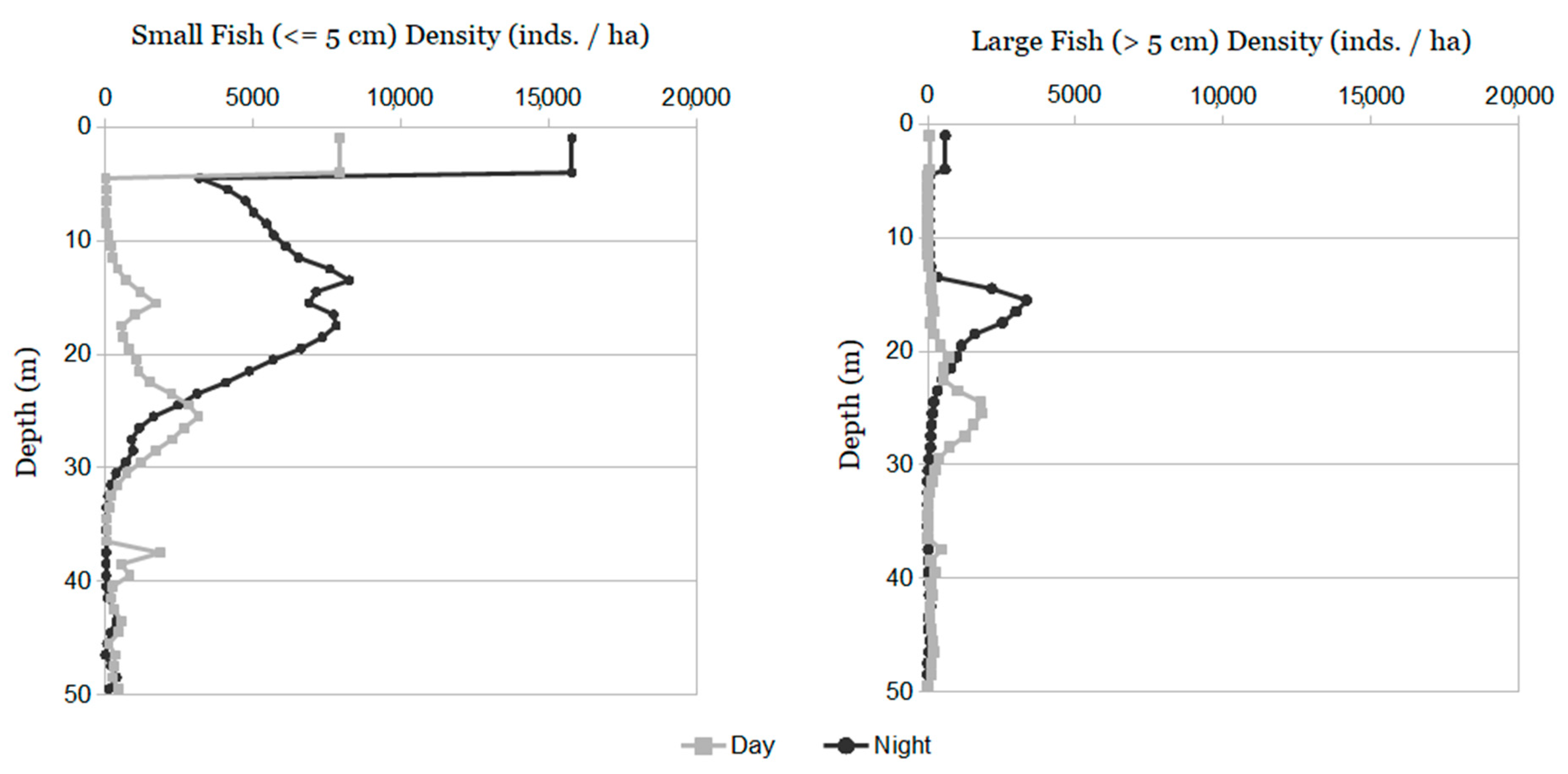
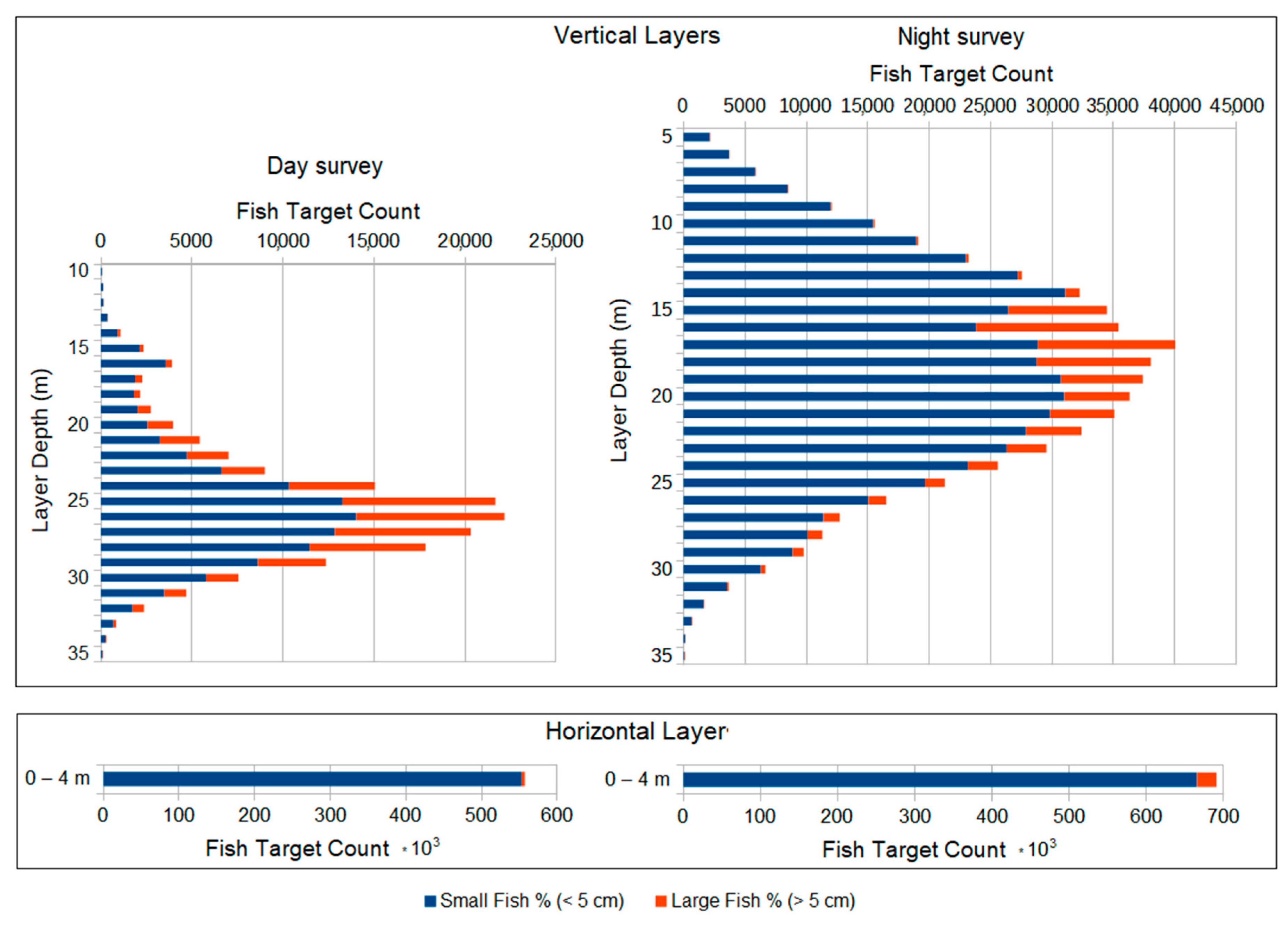
4.2. Fish Size Composition and Distribution
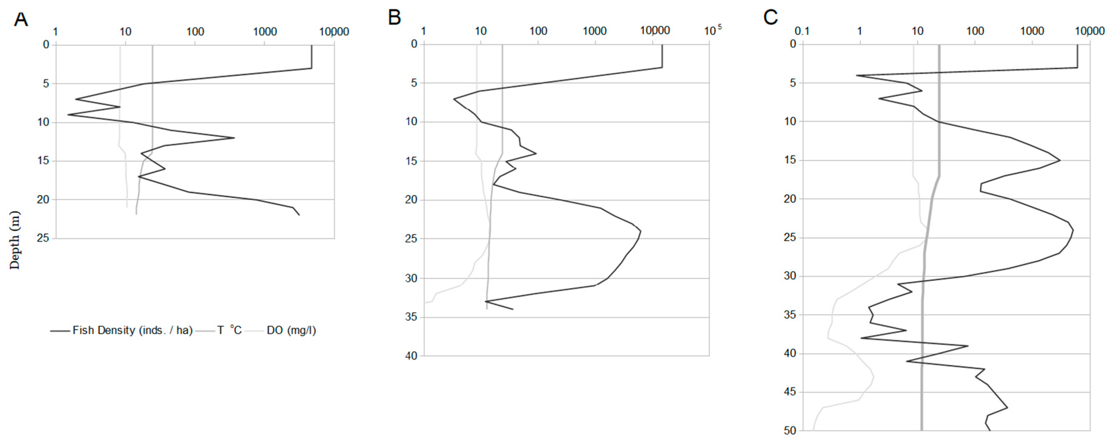
4.3. Temperature and Oxygen Stratification
5. Discussion
Supplementary Materials
Author Contributions
Funding
Acknowledgments
Conflicts of Interest
References
- Arlinghaus, R.; Mehner, T.; Cowx, I.G. Reconciling traditional inland fisheries management and sustainability in industrialized countries, with emphasis on Europe. Fish Fish. 2002, 3, 261–316. [Google Scholar] [CrossRef]
- FAO. Fisheries Management. The Ecosystem Approach to Fisheries; FAO Technical Guidelines for Responsible Fisheries No. 4; FAO: Rome, Italy, 2003. [Google Scholar]
- Oliveira, A.G.; Gomes, L.C.; Latin, J.D.; Agostinho, A.A. Implications of using a variety of fishing strategies and sampling techniques across different biotopes to determine fish species composition and diversity. Nat. Conserv. 2014, 12, 112–117. [Google Scholar] [CrossRef] [Green Version]
- Jackson, D.A.; Harvey, H.H. Qualitative and quantitative sampling of lake fish communities. Can. J. Fish. Aquat. Sci. 1997, 54, 2807–2813. [Google Scholar] [CrossRef]
- Winfield, I.J.; Fletcher, J.M.; James, J.B.; Bean, C.W. Assessment of fish populations in still waters using hydroacoustics and survey gill netting: Experiences with Arctic charr (Salvelinus alpinus) in the UK. Fish. Res. 2009, 96, 30–38. [Google Scholar] [CrossRef]
- Mouratidis, A.; Sarti, F. Flash-flood monitoring and damage assessment with SAR data: Issues and future challenges for earth observation from space sustained by case studies from the Balkans and Eastern Europe. Lect. Notes Geoinf. Cartogr. 2013, 199659, 125–136. [Google Scholar]
- Perivolioti, T.M.; Tušer, M.; Frouzova, J.; Znachor, P.; Rychtecký, P.; Mouratidis, A.; Terzopoulos, D.; Bobori, D. Estimating Environmental Preferences of Freshwater Pelagic Fish Using Hydroacoustics and Satellite Remote Sensing. Water 2019, 11, 2226. [Google Scholar] [CrossRef] [Green Version]
- Simmonds, J.; MacLennan, D. Fisheries Acoustics. Theory and Practice, 2nd ed.; Blackwell Publishing: Oxford, UK, 2005. [Google Scholar]
- Guillard, J.; Lebourges-Daussy, A.; Balk, H.; Colon, M.; Jóźwik, A.; Godlewska, M. Comparing hydroacoustic fish stock estimates in the pelagic zone of temperate deep lakes using three sound frequencies (70, 120, 200 kHz). Inland Waters 2014, 4, 435–444. [Google Scholar] [CrossRef]
- Godlewska, M.; Swierzowski, A.; Winfield, I.J. Hydroacoustics as a tool for studies of fish and their habitat. Int. J. Ecohydrol. Hydrobiol. 2004, 4, 417–427. [Google Scholar]
- Baran, R.; Jůza, T.; Tušer, M.; Balk, H.; Blabolil, P.; Čech, M.; Draštík, V.; Frouzova, J.; Jayasinghe, A.; Koliada, I.; et al. A novel upward-looking hydroacoustic method for improving pelagic fish surveys. Sci. Rep. 2017, 7, 1–12. [Google Scholar] [CrossRef]
- Draštík, V.; Godlewska, M.; Balk, H.; Clabburn, P.; Kubečka, J.; Morrissey, E.; Hatley, J.; Winfield, I.; Mrkvička, T.; Guillard, J. Fish hydroacoustic survey standardization: A step forward based on comparisons of methods and systems from vertical surveys of a large deep lake. Limnol. Oceanogr. Methods 2007, 15, 836–846. [Google Scholar] [CrossRef]
- Edgerton, J.P.; Johnson, A.F.; Turner, J.; LeVay, L.; Mascareñas-Osorio, I.; Aburto-Oropeza, O. Hydroacoustics as a tool to examine the effects of Marine Protected Areas and habitat type on marine fish communities. Sci. Rep. 2018, 8, 47. [Google Scholar] [CrossRef] [PubMed] [Green Version]
- Water Quality—Guidance on the Estimation of Fish Abundance with Mobile Hydroacoustic Methods; CEN. 2014. CEN/TC 230 EN 15910:2014; Comité Européen de Normalisation (European Committee for Standardization): Brussels, Belgium, 2014; 42p.
- Pollom, R.A.; Rose, G.A. A global review of the spatial, taxonomic, and temporal scope of freshwater fisheries hydroacoustics research. Environ. Rev. 2016, 24, 333–347. [Google Scholar] [CrossRef]
- Darwall, W.; Carrizo, S.; Numa, C.; Barrios, V.; Freyhof, J.; Smith, K. Freshwater Key Biodiversity Areas in the Mediterranean Basin Hotspot: Informing Species Conservation and Development Planning in Freshwater Ecosystems; IUCN: Cambridge, UK, 2014. [Google Scholar]
- Encina, L.; Rodriguez-Ruiz, A.; Granado-Lorencio, C. Distribution of common carp in a Spanish reservoir in relation to thermal loading from a nuclear power plant. J. Therm. Biol. 2008, 33, 444–450. [Google Scholar] [CrossRef]
- Georgakarakos, S.; Kitsiou, D. Mapping abundance distribution of small pelagic species applying hydroacoustics and Co-Kriging techniques. In Essential Fish Habitat Mapping in the Mediterranean; Springer: Dordrecht, The Netherlands, 2018. [Google Scholar]
- Tsagkarakis, K.; Giannoulaki, M.; Pyrounaki, M.M.; Machias, A. Species identification of small pelagic fish schools by means of hydroacoustics in the Eastern Mediterranean Sea. Mediterr. Mar. Sci. 2015, 16, 151–161. [Google Scholar] [CrossRef] [Green Version]
- Bobori, D.C.; Economidis, P.S. Freshwater fishes of Greece: Their biodiversity, fisheries and habitats. Aquat. Ecosyst. Health Manag. 2006, 9, 407–418. [Google Scholar] [CrossRef]
- Economou, A.N.; Giakoumi, S.; Vardaka, L.; Barbieri, R.; Stoumboudi, M.Τ.; Zogaris, S. The freshwater ichthyofauna of Greece-an update based on a hydrographic basin survey. Mediterr. Mar. Sci. 2007, 8, 91–166. [Google Scholar] [CrossRef] [Green Version]
- Economidis, P.S. Check List of Freshwater Fishes of Greece: Recent Status of Threats and Protection; Hellenic Society for the Protection of Nature: Athens, Greece, 1991. [Google Scholar]
- Golani, D.; Shefler, D.; Gelman, A. Aspects of growth and feeding habits of the adult European eel (Anguilla anguilla) in Lake Kinneret (Lake Tiberias), Israel. Aquaculture 1988, 74, 349–354. [Google Scholar] [CrossRef]
- Iliadou, K.; Ondrias, I. Biology and morphology of Parasilurus aristotelis (Agassiz, 1856) (Pisces Cypriniformes, Siluridae) in lakes Lysimachia and Trichonis of western Greece. Biol. GalloHellenica 1986, 11, 207–238. (In Greek) [Google Scholar]
- Daoulas, C.; Kattoulas, M. Reproductive biology of Rutilus rubilio (Bonaparte, 1837) in Lake Trichonis. Hydrobiology 1985, 124, 49–55. [Google Scholar] [CrossRef]
- Daoulas, C.; Economou, A.N.; Psarras, T.; Barbieri-Tseliki, R. Reproductive strategies and early development of three freshwater gobies. J. Fish Biol. 1993, 42, 749–776. [Google Scholar] [CrossRef]
- Leonardos, I.D. Life history traits of Scardinius acarnanicus (Economidis, 1991) (Pisces: Cyprinidae) in two Greek lakes (Lysimachia and Trichonis). J. Appl. Ichthyol. 2004, 20, 258–264. [Google Scholar] [CrossRef]
- Leonardos, I.D.; Kagalou, I.; Triantafyllidis, A.; Sinis, A. Life history traits of ylikiensis roach (Rutilus ylikiensis) in two Greek lakes of different trophic state. J. Freshw. Ecol. 2005, 20, 715–722. [Google Scholar] [CrossRef]
- Leonardos, I.D. Ecology and exploitation pattern of a landlocked population of sand smelt, Atherina boyeri (Risso 1810), in Trichonis Lake (western Greece). J. Appl. Ichthyol. 2001, 17, 262–266. [Google Scholar] [CrossRef] [Green Version]
- Economou, A.N.; Daoulas, C.H.; Psarras, T.; Barbieri-Tseliki, R. Freshwater larval fish from lake Trichonis (Greece). J. Fish Biol. 1994, 45, 17–35. [Google Scholar] [CrossRef]
- Froese, R.; Pauly, D. Fishbase. Available online: www.fishbase.in (accessed on 1 April 2020).
- Leonardos, I.; Kokkinidou, A.; Agiannitopoulos, A.; Giris, S. Population structure and reproductive strategy of an endemic species Scardinius acarnanicus (Stephanidis, 1939) in two W. Greece Lakes (Lysimachia and Trichonis). In Proceedings of the Ninth Ichthyological Congress, Messolonghi, Greece, 20–23 January 2000; pp. 137–140, (In Greek with English Abstract). [Google Scholar]
- Kehayias, G.; Doulka, E. Trophic state evaluation of a large Mediterranean lake utilizing abiotic and biotic elements. J. Environ. Prot. 2014, 5, 17–28. [Google Scholar] [CrossRef] [Green Version]
- Luther, H.; Rzoska, J. Project Aqua: (A Source Book of Inland Waters Proposed for Conservation); Blackwell Scientific Publications: Oxford & Edinburgh, UK, 1972. [Google Scholar]
- Mouratidis, A.; Ampatzidis, D. European Digital Elevation Model Validation against Extensive Global Navigation Satellite Systems Data and Comparison with SRTM DEM and ASTER GDEM in Central Macedonia (Greece). ISPRS Int. J. Geo-Inf. 2019, 8, 108. [Google Scholar] [CrossRef] [Green Version]
- Mouratidis, A.; Karadimou, G.; Ampatzidis, D. Extraction and Validation of Geomorphological Features from EU-DEM in the Vicinity of the Mygdonia Basin, Northern Greece. Proc. IOP Conf. Ser. Earth Environ. Sci. 2017, 95, 032009. [Google Scholar] [CrossRef]
- Draštík, V.; Kubečka, J.; Čech, M.; Frouzova, J.; Říha, M.; Juza, T.; Tušer, M.; Jarolím, O.; Prchalová, M.; Peterka, J.; et al. Hydroacoustic estimates of fish stocks in temperate reservoirs: Day or night surveys? Aquat. Living Resour. 2009, 22, 69–77. [Google Scholar]
- Aglen, A. Random errors of acoustic fish abundance estimates in relation to the survey grid density applied. FAO Fish. Rep. 1983, 300, 293–298. [Google Scholar]
- Guillard, J.; Vergès, C. The repeatability of fish biomass and size distribution estimates obtained by hydroacoustic surveys using various sampling strategies and statistical analyses. Int. Rev. Hydrobiol. 2007, 92, 605–617. [Google Scholar] [CrossRef]
- Demer, D.A.; Berger, L.; Bernasconi, M.; Bethke, E.; Boswell, K.; Chu, D.; Domokos, R.; Dunford, A.; Fassler, S.; Gauthier, S.; et al. Calibration of Acoustic Instruments; ICES Cooperative Research Report, No. 326; ICES: Copenhagen, Denmark, 2015; p. 133. [Google Scholar]
- Balk, H.; Lindem, T. Sonar4, Sonar5, Sonar6 Post Processing Systems, Operator Manual Version (5.9.6); SIMRAD: Oslo, Norway, 2006. [Google Scholar]
- Love, R.H. Dorsal-aspect target strength of an individual fish. J. Acoust. Soc. Am. 1971, 49, 816–823. [Google Scholar] [CrossRef]
- Frouzova, J.; Kubecka, J.; Balk, H.; Frouz, J. Target strength of some European fish species and its dependence on fish body parameters. Fish. Res. 2005, 75, 86–96. [Google Scholar] [CrossRef]
- Frouzova, J.; Kubečka, J.; Matěna, J. Acoustic scattering properties of freshwater invertebrates. In Proceedings of the Seventh European Conference on Underwater Acoustic (ECUA 2004), Delft University of Technology, Delft, The Netherlands, 5–8 July 2004; pp. 319–324. [Google Scholar]
- Kubečka, J.; Wittingerová, M. Horizontal beaming as a crucial component of acoustic fish stock assessment in freshwater reservoirs. Fish. Res. 1998, 35, 99–106. [Google Scholar] [CrossRef]
- Sawada, K.; Furusawa, M.; Williamson, N.J. Conditions for the precise measurement of fish target strength in situ. J. Mar. Acoust. Soc. Jpn. 1993, 2, 73–79. [Google Scholar] [CrossRef]
- Lee, S.; Wolberg, G.; Shin, S.Y. Scattered data interpolation with multilevel B-splines. IEEE Trans. Vis. Comput. Graph. 1997, 3, 228–244. [Google Scholar] [CrossRef] [Green Version]
- Nürnberg, G.K. Quantified hypoxia and anoxia in lakes and reservoirs. Sci. World J. 2004, 4, 42–54. [Google Scholar] [CrossRef] [Green Version]
- Johannesson, K.A.; Mitson, R.B. Fisheries Acoustics. A Practical Manual for Aquatic Biomass Estimation; FAO Fisheries Technical Paper: Rome, Italy, 1992. [Google Scholar]
- Boswell, K.M.; Wilson, M.P.; Wilson, C.A. Hydroacoustics as a tool for assessing fish biomass and size distribution associated with discrete shallow water estuarine habitats in Louisiana. Estuaries Coasts 2007, 30, 607–617. [Google Scholar] [CrossRef]
- Emmrich, M.; Winfield, I.J.; Guillard, J.; Rustadbakken, A.; Verges, C.; Volta, P.; Jeppesen, E.; Lauridsen, T.L.; Brucet, S.; Holmgren, K.; et al. Strong correspondence between gillnet catch per unit effort and hydroacoustically derived fish biomass in stratified lakes. Freshw. Biol. 2012, 57, 2436–2448. [Google Scholar] [CrossRef] [Green Version]
- Čech, M.; Kubečka, J.; Frouzová, J.; Draštík, V.; Kratochvíl, M.; Matěna, J.; Hejzlar, J. Distribution of the bathypelagic perch fry layer along the longitudinal profile of two large canyon-shaped reservoirs. J. Fish Biol. 2007, 70, 141–154. [Google Scholar]
- Neilson, J.D.; Perry, R.I. Diel vertical migrations of marine fishes: An obligate or facultative process? Adv. Mar. Biol. 1990, 26, 115–168. [Google Scholar]
- Helfman, G.S.; Winkelman, D.L. Threat sensitivity in bicolor damselfish: Effects of sociality and body size. Ethology 1997, 103, 369–383. [Google Scholar] [CrossRef]
- Appenzeller, A.R.; Leggett, W.C. Bias in hydroacoustic estimates of fish abundance due to acoustic shadowing: Evidence from day–night surveys of vertically migrating fish. Can. J. Fish. Aquat. Sci. 1992, 49, 2179–2189. [Google Scholar] [CrossRef]
- Parker-Stetter, S.L. Standard Operating Procedures for Fisheries Acoustic Surveys in the Great Lakes; Great Lakes Fisheries Commission Special Publication, 09–01: Ann Arbor, MI, USA, 2009. [Google Scholar]
- Kagalou, I.; Economidis, G.; Leonardos, I.; Papaloukas, C. Assessment of a Mediterranean shallow lentic ecosystem (Lake Pamvotis, Greece) using benthic community diversity: Response to environmental parameters. Limnologica 2006, 36, 269–278. [Google Scholar] [CrossRef] [Green Version]
- Wheeland, L.J.; Rose, G.A. Quantifying fish avoidance of small acoustic survey vessels in boreal lakes and reservoirs. Ecol. Freshw. Fish 2015, 24, 67–76. [Google Scholar] [CrossRef]
- Doulka, E.; Kehayias, G. Seasonal vertical distribution and diel migration of zooplankton in a temperate stratified lake. Biologia 2011, 66, 308–319. [Google Scholar] [CrossRef]
- Godlewska, M.; Świerzowski, A. Hydroacoustical parameters of fish in reservoirs with contrasting levels of eutrophication. Aquat. Living Resour. 2003, 16, 167–173. [Google Scholar] [CrossRef]
- Breitburg, D.L.; Rose, K.A.; Cowan, J.H., Jr. Linking water quality to larval survival: Predation mortality of fish larvae in an oxygen-stratified water column. Mar. Ecol. Prog. Ser. 1999, 178, 39–54. [Google Scholar] [CrossRef] [Green Version]


| Lake Location | Latitude (deg) | Longitude (deg) | Sampled Depth Range (m) |
|---|---|---|---|
| Sampling point S1 | 38.58625 | 21.48000 | 22 |
| Sampling point S2 | 38.57250 | 21.48301 | 34 |
| Sampling point S3 | 38.53671 | 21.61033 | 50 |
| Sampling Point S1 | Sampling Point S2 | Sampling Point S3 | ||||
|---|---|---|---|---|---|---|
| Temperature | Dissolved Oxygen | Temperature | Dissolved Oxygen | Temperature | Dissolved Oxygen | |
| R | −0.56 | 0.54 | −0.52 | 0.53 | 0.018 | 0.61 |
| R2 | 0.31 | 0.29 | 0.27 | 0.28 | 0.00032 | 0.37 |
| p-value | 0.013 | 0.018 | 0.0026 | 0.0023 | 0.91 | 5.9 × 10⁻⁶ |
| DF | 17 | 17 | 29 | 29 | 45 | 45 |
© 2020 by the authors. Licensee MDPI, Basel, Switzerland. This article is an open access article distributed under the terms and conditions of the Creative Commons Attribution (CC BY) license (http://creativecommons.org/licenses/by/4.0/).
Share and Cite
Perivolioti, T.-M.; Frouzova, J.; Tušer, M.; Bobori, D. Assessing the Fish Stock Status in Lake Trichonis: A Hydroacoustic Approach. Water 2020, 12, 1823. https://doi.org/10.3390/w12061823
Perivolioti T-M, Frouzova J, Tušer M, Bobori D. Assessing the Fish Stock Status in Lake Trichonis: A Hydroacoustic Approach. Water. 2020; 12(6):1823. https://doi.org/10.3390/w12061823
Chicago/Turabian StylePerivolioti, Triantafyllia-Maria, Jaroslava Frouzova, Michal Tušer, and Dimitra Bobori. 2020. "Assessing the Fish Stock Status in Lake Trichonis: A Hydroacoustic Approach" Water 12, no. 6: 1823. https://doi.org/10.3390/w12061823